The effect of non tightness on Bayesian estimation of PCFGs

The effect of non-tightness on Bayesian estimation of PCFGs

Shay B. Cohen

Department of Computer Science Columbia University

[email protected]

Mark Johnson Department of Computing

Macquarie University

[email protected]

Abstract

Probabilistic context-free grammars have the unusual property of not always defining tight distributions (i.e., the sum of the “probabili-ties” of the trees the grammar generates can be less than one). This paper reviews how this non-tightness can arise and discusses its im-pact on Bayesian estimation of PCFGs. We begin by presenting the notion of “almost ev-erywhere tight grammars” and show that lin-ear CFGs follow it. We then propose three dif-ferent ways of reinterpreting non-tight PCFGs to make them tight, show that the Bayesian es-timators in Johnson et al. (2007) are correct under one of them, and provide MCMC sam-plers for the other two. We conclude with a discussion of the impact of tightness empiri-cally.

1 Introduction

Probabilistic Context-Free Grammars (PCFGs) play a special role in computational linguistics because they are perhaps the simplest probabilistic models of hierarchical structures. Their simplicity enables us to mathematically analyze their properties to a de-tail that would be difficult with linguistically more accurate models. Such analysis is useful because it is reasonable to expect more complex models to ex-hibit similar properties as well.

The problem of inferring PCFG rule probabili-ties from training data consisting of yields or strings alone is interesting from both cognitive and engi-neering perspectives. Cognitively it is implausible that children can perceive the parse trees of the lan-guage they are learning, but it is more reasonable to assume that they can obtain the terminal strings or yield of these trees. Unsupervised methods for learning a grammar from terminal strings alone is also interesting from an engineering perspective be-cause such training data is cheap and plentiful, while

the manually parsed data required by supervised methods are expensive to produce and relatively rare.

Cohen and Smith (2012) show that inferring PCFG rule probabilities from strings alone is com-putationally intractable, so we should not expect to find an efficient, general-purpose algorithm for the unsupervised problem. Instead, approximation algo-rithms are standardly used. For example, the Inside-Outside (IO) algorithm efficiently implements the Expectation-Maximization (EM) procedure for ap-proximating a Maximum Likelihood estimator (Lari and Young, 1990). Bayesian estimators for PCFG rule probabilities have also been attracting attention because they provide a theoretically-principled way of incorporating prior information. Kurihara and Sato (2006) proposed a Variational Bayes estima-tor based on a mean-field approximation, and John-son et al. (2007) proposed MCMC samplers for the posterior distribution over rule probabilities and the parse trees of the training data strings.

PCFGs have the interesting property (which we expect most linguistically more realistic models to also possess) that the distributions they define are not always properly normalized or “tight”. In a non-tight PCFG the partition function (i.e., sum of the “probabilities” of all the trees generated by the PCFG) is less than one. (Booth and Thompson, 1973, called such non-tight PCFGs “inconsistent”, but we follow Chi and Geman (1998) in calling them “non-tight” to avoid confusion with the consis-tency of statistical estimators). Chi (1999) showed that renormalized nontight PCFGs (which he called “Gibbs CFGs”) define the same class of distributions over trees as do tight PCFGs with the same rules, and provided an algorithm for mapping any PCFG to a tight PCFG with the same rules that defines the same distribution over trees.

affect the inference of PCFGs? Chi and Geman (1998) studied the question for Maximum Likeli-hood (ML) estimation, and showed that ML esti-mates are always tight for both the supervised case (where the input consists of parse trees) and the un-supervised case (where the input consists of yields or terminal strings). This means that ML estimators can simply ignore issues of tightness, and rest as-sured that the PCFGs they estimate are in fact tight. The situation is more subtle with Bayesian esti-mators. We show that for the special case of linear PCFGs (which include HMMs) with non-degenerate priors the posterior puts zero mass on non-tight PCFGs, so tightness is not an issue with Bayesian estimation of such grammars. However, because all of the commonly used priors (such as the Dirichlet or the logistic normal) assign non-zero probability across the whole probability simplex, in general the posterior may assign zero probability to non-tight PCFGs. We discuss three different possible ap-proaches to this in this paper:

1. theonly-tightapproach, where we modify the prior so it only assigns non-zero probability to tight PCFGs,

2. therenormalizationapproach, where we renor-malize non-tight PCFGs so they define a prob-ability distribution over trees, and

3. the sink-element approach, where we reinter-pret non-tight PCFGs as assigning non-zero probability to a “sink element”, so both tight and non-tight PCFGs are properly normalized.

We show how to modify the Gibbs sampler de-scribed by Johnson et al. (2007) so it produces sam-ples from the posterior distributions defined by the only-tight and renormalization approaches. Perhaps surprisingly, we show that Gibbs sampler as defined by Johnson et al. actually produces samples from the posterior distributions defined by the sink-element approach.

We conclude by studying the effect of requiring tightness on the estimation of some simple PCFGs. Because the Bayesian posterior converges around the (tight) ML estimate as the size of the data grows, requiring tightness only seems to make a difference with highly biased priors or with very small training corpora.

2 PCFGs and tightness

LetG = (T, N, S, R) be a Context-Free Grammar in Chomsky normal form with no useless produc-tions, whereT is a finite set ofterminal symbols,N is a finite set ofnonterminal symbols(disjoint from T),S ∈N is a distinguished nonterminal called the start symbol, andRis a finite set ofproductionsof the formA→B CorA→w, whereA, B, C∈N andw ∈T. In what follows we useβ as a variable ranging over(N×N)∪T.

AProbabilistic Context-Free Grammar(G,Θ)is a pair consisting of a context-free grammarGand a real-valued vectorΘof length|R|indexed by pro-ductions, whereθA→β is theproduction probability

associated with the production A → β ∈ R. We require thatθA→β ≥0and that for all nonterminals

A ∈ N, P

A→β∈RAθA→β = 1, whereRA is the subset of rulesRexpanding the nonterminalA.

A PCFG(G,Θ)defines a measureµΘover trees

tas follows:

µΘ(t) =

Y

r∈R

θfr(t)

r

where fr(t) is the number of times the production

r=A→β ∈Ris used in the derivation oft. Thepartition functionZ or measure of all possi-ble trees is:

Z(Θ) = X

t0_∈T Y

r∈R

θfr(t0)

r

where T is the set of all (finite) trees generated by G. A PCFG is tight iff the partition function Z(Θ) = 1. In this paper we useΘ⊥ to denote the set of rule probability vectorsΘfor whichGis non-tight. Nederhof and Satta (2008) survey several al-gorithms for computingZ(Θ), and hence for deter-mining whether a PCFG is tight.1

Non-tightness can arise in very simple PCFGs, such as the “Catalan” PCFG S → S S|a. This grammar produces binary trees where all internal

1

nodes are labeled asS and the yield of these trees is a sequence of as. If the probability of the rule S →S S is greater than 0.5 then this PCFG is non-tight.

Perhaps the most straight-forward way to under-stand this non-tightness is to view this grammar as defining a branching process where anScan either “reproduce” with probability θS→S S or “die out”

with probabilityθS→a. WhenθS→S S > θS→athe

Snodes reproduce at a faster rate than they die out, so the derivation has a non-zero probability of end-lessly rewriting (Atherya and Ney, 1972).

3 Bayesian inference for PCFGs

The goal of Bayesian inference for PCFGs is to in-fer a posterior distribution over the rule probability vectors Θ given observed data D. This posterior distribution is obtained by combining the likelihood P(D|Θ)with a prior distributionP(Θ)overΘ us-ing Bayes Rule.

P(Θ|D)∝P(D|Θ) P(Θ)

We now formally define the three approaches to handling non-tightness mentioned earlier:

the only-tight approach: we only permit priors

whereP(Θ⊥) = 0, i.e., we insist that the prior assign zero mass to non-tight rule probability vectors, soZ= 1. This means we can define:

P(t|Θ) =µΘ(t)

the renormalization approach: we renormalize

non-tight PCFGs by dividing by the partition function:

P(t|Θ) = 1

Z(Θ)µΘ(t) (1)

the sink-element approach: we redefine our

prob-ability distribution so its domain is a setT0 = T ∪{⊥}, whereT is the set of (finite) trees gen-erated byGand⊥ 6∈ T is a new element that serves as a “sink state” to which the “missing

mass”1−Z(Θ)is assigned. Then we define:2

P(t|Θ) =

µΘ(t) ift∈ T

1−Z(Θ) ift=⊥

With this in hand, we can now define the likeli-hood term. We consider two types of data Dhere. In thesupervised settingthe dataDconsists of a cor-pus of parse treesD= (t1, . . . , tn)where each tree

tiis generated by the PCFGG, so

P(D|Θ) =

n

Y

i=1

P(ti|Θ)

In theunsupervised settingthe dataDconsists of a corpus of stringsD = (w1, . . . , wn) where each

stringwi is the yield of one or more trees generated

byG. In this setting

P(D|Θ) =

n

Y

i=1

P(wi|Θ),where:

P(w|Θ) = X

t∈T:yield(t)=w

P(t|Θ)

4 The special case of linear PCFGs

One way to handle the issue of tightness is to iden-tify a family of CFGs for which practically any pa-rameter setting will yield a tight PCFG. This is the focus of this section, in which we identify a subset of CFGs, which are “almost everywhere” tight. This family of CFGs includes many of the CFGs used in NLP applications.

We cannot expect that a CFG will yield a tight PCFG for any assignment to the rule probabilities (i.e. thatΘ⊥=∅). Even in simple cases, such as the grammar S → S|a, the assignment of probability 1 toS → S and 0 to the other rule renders the S nonterminal useless, and places all of the probability

2

This definition of a distribution over trees can be induced by a tight PCFG with a special⊥symbol in its vocabulary. GivenG, the first step is to create a tight grammarG0using the

renormalization approach. Then, a new start symbol is added to

G0,S0, and also rulesS0 →S(whereSis the old start symbol

inG0) andS0 → ⊥. The first rule is given probabilityZ(Θ)

and the second rule is given probability1−Z(Θ). It can be then readily shown that the new tight PCFGG0induces a

dis-tribution over trees just like in Eq. 3, only with additionalS0on

mass on infinite structures of the form S → S → S →. . ..

However, we can weaken our requirement so that the cases in which parameter assignment yields a non-tight PCFG are rare, or have measure zero. To put it more formally, we say that a prior P(Θ) is “tight almost everywhere forG” if

P(Θ⊥) = Z

Θ∈Θ⊥

P(Θ)dΘ = 0.

We now provide a sufficient condition (linearity) for CFGs under which they are tight almost every-where with any continuous prior.

For a nonterminalA∈N andβ ∈(N ∪T)∗, we useA⇒k_{βto denote thatAcan be re-written using}

a sequence of rules fromR to the sentential formβ inkderivation steps. We useA⇒+_{βto denote that}

there exists ak >0such thatA⇒k _β.

Definition 1 A context-free grammarG islinear if

there are noA∈N such that3

A⇒+. . . A . . . A . . . .

Let L(A) = {w|A ⇒∗ w, w ∈ T∗}. Define G(A)to be the grammarGwhereS is replaced by A. We assume Ghas no useless nonterminals, i.e. each nonterminal A participates in some complete tree derivation (but it could potentially have prob-ability0). Useless nonterminals can always be re-moved from a grammar without changing the lan-guage generated by the grammar.

Definition 2 A nonterminalA∈N in a

probabilis-tic context-free grammar G with parameters Θ is nonterminatingif:

• Ais recursive: there is aβsuch thatA ⇒+ _β

andAappears inβ.

• PG(A)(L(A)) =

P

w∈L(A)PG(A)(w) = 0.

Lemma 1 A linear PCFG G with parameters Θ

which does not have any nonterminating nontermi-nals is tight.

3

Note that this definition of linear CFGs deviates from the traditional definition, which states that a PCFG is linear if the right handside of each rule includes at most one nonterminal. The traditional definition implies Definition 1.

Proof:Our proof relies on the properties of a certain |N| × |N|matrixM where:

MAB =

X

A→β∈RA

n(β, B)θA→β

wheren(β, B) is the number of appearances of the nonterminalB in the sequenceβ. MAB is the

ex-pected number of B nonterminals generated from anAnonterminal in one single derivational step, so [Mk]AB is the expected number ofB nonterminals

generated from anAnonterminal in ak-step deriva-tion (Wetherell, 1980).

Since M is a non-negative matrix, under some regularity conditions, the Frobenius-Perron theorem states that the largest eigenvalue of this matrix (in absolute value) is a real number. Let this eigenvalue be denoted byλ.

A PCFG is called “subcritical” if λ < 1and su-percritical ifλ > 1. Then, in turn, a PCFG is tight if it is subcritical. It is not tight if it is supercriti-cal. The case ofλ= 1is a borderline case that does not give sufficient information to know whether the PCFG is tight or not. In the Bayesian case, for a continuous prior such as the Dirichlet prior, this bor-derline case will have measure zero under the prior.

Now let A ∈ N. Since the grammar is linear, there is no derivationA ⇒+ _{. . . A . . . A . . ..}

There-fore, any derivation of the formA⇒+_{. . . A . . .}

in-cludesA on the right hand-side exactly once. Be-cause the grammar has no nonterminating nontermi-nals, the probability of such a derivation is strictly smaller than 1.

For eachA∈N, define:

pA=

X

β=...A...

P(A⇒|N|β|Θ).

Since A is not useless, thenpA < 1. Therefore

q= maxApA<1. Since any derivation of lengthk

of the formA⇒. . . A . . .can be decomposed to at

least k

2|N| cycles that start at a terminalB ∈N and end in the same nonterminalB ∈N, it holds that:

[Mk]AA≤q

k

2|N| k→∞_{→ 0.}

Proposition 1 Any continuous priorP(Θ)on a lin-ear grammarGis tight almost everywhere forG.

Proof: LetG be a linear grammar. With a contin-uous prior, the probability ofG getting parameters from the prior which yield a useless non-terminal is 0 – it would require setting at least one rule in the grammar with rule probability which is exactly 1. Therefore, with probability 1, the parameters taken from the prior yield a PCFG which is linear and does not have nonterminating nonterminals. According to Lemma 1, this means the PCFG is tight.

Deciding whether a grammar G is linear can be done in polynomial time using the construction from Bar-Hillel et al. (1964). We can first eliminate the differences between nonterminals and terminal sym-bols by adding a ruleA→ cAfor each nonterminal

A ∈N, after extending the set of terminal symbols A with {cA|A ∈ N}. Let GA be the grammar G

with the start symbol being replaced withA. We can then intersect the grammarGAwith the regular

lan-guageT∗cAT∗cAT∗(for each nonterminalA∈N).

If for any nonterminalA the intersection is not the empty set (with respect to the language that the in-tersection generates), then the grammar is not linear. Checking whether the intersection is the empty set or not can be done in polynomial time.

We conclude this section by remarking that many of the models used in computational linguistics are in fact equivalent to linear PCFGs, so continuous Bayesian priors are almost everywhere tight. For ex-ample, HMMs and many kinds of “stacked” finite-state machines are equivalent to linear PCFGs, as are the example PCFGs given in Johnson et al. (2007) to motivate the MCMC estimation procedures.

5 Dirichlet priors

The first step in Bayesian inference is to specify a prior on Θ. In the rest of this paper we take P(Θ) to be a product of Dirichlet distributions, with one distribution for each non-terminalA ∈ N, as this turns out to simplify the computations considerably. The prior is parameterized by a positive real valued vectorαindexed by productionsR, so each produc-tion probabilityθA→β has a corresponding Dirichlet

parameter αA→β. As before, letRA be the set of

productions in R with left-hand sideA, and letθA

andαArefer to the component subvectors ofθ and

α respectively indexed by productions inRA. The

Dirichlet priorP(Θ|α)is:

P(Θ|α) = Y

A∈N

PD(ΘA|αA),

where

PD(ΘA|αA) =

1 C(αA)

Y

r∈RA θαr−1

r and

C(αA) =

Q

r∈RAΓ(αr) Γ(P

r∈RAαr)

where Γ is the generalized factorial function and C(α)is a normalization constant that does not de-pend onΘA.

Dirichlet priors are useful because they are con-jugateto the multinomial distribution, which is the building block of PCFGs. Ignoring issues of tight-ness for the moment and settingP(t|Θ) = µΘ(t),

this means that in the supervised setting the poste-rior distributionP(Θ|t, α)given a set of parse trees t = (t1, . . . , tn)is also a product of Dirichlets

dis-tribution.

P(Θ|t, α)∝P(t|Θ) P(Θ|α)

∝ Y

r∈R

θfr(t)

r

! Y

r∈R

θαr−1

r

!

= Y

r∈R

θfr(t)+αr−1

r

which is a product of Dirichlet distributions with pa-rametersf(t) +α, wheref(t) is the vector of rule counts intindexed byr∈R. We can thus write:

P(Θ|t, α) = P(Θ|f(t) +α)

which makes it clear that the rule counts are directly added to the parameters of the prior to produce the parameters of the posterior.

6 Inference in the supervised setting

We first discuss Bayesian inference in the supervised setting, as inference in the unsupervised setting is based on inference for the supervised setting. For each of the three approaches to non-tightness we provide an algorithm that characterizes the poste-riorP(Θ |t), wheret= (t1, . . . , tn)is a sequence

Input: GrammarG, vector of treest, vector of hyperparametersα, previous parametersΘ0. Result: A vector of parametersΘ

repeat

drawθfrom products of Dirichlet with hyperparametersα+f(t)

untilΘis tight forG; returnΘ

Algorithm 1:An algorithm for generating samples

fromP(Θ|t, α)for the only-tight approach.

Input: GrammarG, vector of treest, vector of hyperparametersα, previous rule parameters

Θ0.

Result: A vector of parametersΘ

draw a proposalΘ∗from a product of Dirichlets with parametersα+f(t).

draw a uniform numberufrom[0,1]. ifu <min{1, Z(Θ(i−1)_)/Z(Θ∗₎n

}returnΘ∗. returnΘ0.

Algorithm 2:One step of Metropolis-Hastings

al-gorithm for generating samples from P(Θ | t, α) for the renormalization approach.

6.1 The only-tight approach

The “only-tight” approach requires that the prior as-sign zero mass to non-tight rule probability vectors Θ⊥. One way to define such a distribution is to restrict the domain of an existing prior distribution with the set of tightΘand renormalize. In more de-tail, ifP(Θ) is a prior over rule probabilities, then its renormalization is the priorP0 defined as:

P0(Θ) = P(Θ)I(Θ∈/Θ

⊥₎

Z(Θ⊥₎ . (2)

whereZ(Θ⊥) =R

ΘP(Θ)I(Θ∈/Θ ⊥_)dΘ.

Perhaps surprisingly, it turns out that ifP(Θ) be-longs to a family of conjugate priors, then P0(Θ) also belongs to a (different) family of conjugate pri-ors as well.

Proposition 2 LetP(Θ|α)be a prior with

hyperpa-rameters α over the parameters of G such that P is conjugate to the grammar likelihood. Then P0, defined in Eq.2, is conjugate to the grammar likeli-hood as well.

Proof: Assume that trees t are observed, and the

Input: GrammarG, vector of treest, vector of hyperparametersα, previous parametersΘ0. Result: A vector of parametersΘ

drawΘfrom products of Dirichlet with hyperparametersα+f(t)

returnΘ

Algorithm 3:An algorithm for generating samples

fromP(Θ|t, α)for the sink-state approach.

prior over the grammar parameters is the prior de-fined in Eq. 2. Therefore, the posterior is:

P(Θ|t, α)∝P0(Θ|α)p(t|Θ)

= P(Θ|α)p(t|Θ)I(Θ∈/ Θ

⊥₎

Z(Θ⊥)

∝ P(Θ|t, α)I(Θ∈/ Θ

⊥₎

Z(Θ⊥₎ .

Since P(Θ|α) is a conjugate prior to the PCFG likelihood, then there exists α0 = α0(t) such that P(Θ|t, α) = P0(Θ|α0). Therefore:

P(Θ|t, α)∝ P(Θ|α

0_{)I(Θ∈/ Θ}⊥₎

Z(Θ⊥₎ .

which exactly equalsP0(Θ|α0).

Sampling from the posterior over the parameters given a set of treestis therefore quite simple when assuming the base prior being renormalized is a product of Dirichlets. Algorithm 1 samples from a product of Dirichlets distribution with hyperparam-eters α+f(t) repeatedly, each time checking and rejecting the sample until we obtain a tight PCFG.

The more mass the Dirichlet distribution with hy-perparameters α+f(t) puts on non-tight PCFGs, the more rejections will happen. In general, if the probability mass on non-tight PCFGs isq⊥, then it

would require, on average1/(1−q⊥)samples from

this distribution in order to obtain a tight PCFG.

6.2 The renormalization approach

P(Θ|t) =

n

Y

i=1

µΘ(ti)

Z(Θ) P(Θ|α)

∝ 1

Z(Θ)n P(Θ|α+f(t)). (3)

Note that the factor Z(Θ) depends on Θ, and therefore cannot be absorbed into the constant. Al-gorithm 2 describes a Metropolis-Hastings sampler for sampling from the posterior in Eq. 3 that uses a product of Dirichlets with parametersα+f(t)as a proposal distribution.

In our experiments, we use the algorithm from Nederhof and Satta (2008) to compute the partition function which is needed in Algorithm 2.

6.3 The “sink element” approach

The “sink element” approach does not affect the likelihood (since the probability of a tree t is just the product of the probabilities of the rules used to generate it), nor does it require a change to the prior. (The sink element⊥is not a member of the set of treesT, so it cannot appear in the datat).

This means that the conjugacy argument given at the bottom of section 5 holds in this approach, so the posteriorP(Θ|t, α)is a product of Dirichlets with parametersf(t) +α. Algorithm 3 gives a sampler forP(Θ|t, α)for the sink element approach.

7 Inference in the unsupervised setting Johnson et al. (2007) provide two Markov chain Monte Carlo algorithms for Bayesian inference for PCFG rule probabilities in the unsupervised setting (i.e., where the data consists of a corpus of strings w = (w1, . . . , wn)alone). The algorithms we give

here are based on their Gibbs sampler, which in each iteration first samples parse treest = (t1, . . . , tn),

where eachti is a parse forwi, from P(t | w,Θ),

and then samplesΘfromP(Θ|t, α).

Notice that the conditional distribution P(t | w,Θ)is unaffected in each of our three approaches (the partition functions cancel in the renormaliza-tion approach), so the algorithm for sampling from P(t|w,Θ)given by Johnson et al. applies in each of our three approaches as well.

Johnson et al. ignored tightness and assumed that P(Θ |t, α) is a product of Dirichlets with

parame-Input: GrammarG, vector of hyperparametersα, vector of stringsw= (w1, . . . , wn),

previous rule parametersΘ0. Result: A vector of parametersΘ fori←1tondo

drawtifromP(ti|wi,Θ0) end

use Algorithm 2 to sampleΘgivenG,t,αandΘ0

returnΘ

Algorithm 4: One step of the

Metropolis-within-Gibbs sampler for the renormalization approach.

tersf(t) +α. As we noted in section 6.3, this as-sumption holds for the sink-state approach to non-tightness, so their sampler is in fact correct for the sink-state approach.

In fact, we obtain samplers for the unsupervised setting for each of our approaches by “plugging in” the corresponding sampling algorithm (Eq. 1–3) for P(Θ | t, α) into the generic Gibbs sampler frame-work of Johnson et al.

The one complication is that because we use a Metropolis-Hastings procedure to generate sam-ples from P(Θ | t, α) in the renormalization ap-proach, we use the Metropolis-within-Gibbs pro-cedure given in Algorithm 4 (Robert and Casella, 2004).

8 The expressive power of the three approaches

following sense: any prior used with one of the ap-proaches can be transformed into a different prior that can be used with one of the other approaches, and yield identical posterior over trees conditioned on a string, marginalizing out the parameters.

This does not mean that the three approaches are equivalent, however. In this section we provide a grammar such that with a uniform prior over rule probabilities, the conditional distribution over trees given a fixed string varies under each of the three different approaches.

The grammar we consider has three rules S → S S S|S S|awith probabilitiesθ1, θ2 and1−θ1−

θ2, respectively. TheΘ parameters are required to

satisfyθ1+θ2 ≤1andθi≥0fori= 1,2.

We compute the posterior distribution over parse trees for the stringw=a a a.

The grammar generates three parse trees forw1,

namely: t1= S

S a

S a

S a

t2= S

S a

S S a

S a

t3= S

S S a

S a

S a

The partition function Z for this grammar is the smallest positive root of the cubic equation:

Z=θ1Z3+θ2Z2+ (1−θ1−θ2)

We used Mathematica to find an analytic solution for Z in this equation, obtaining not only an expression for the partition functionZ(Θ) but also identifying the non-tight regionΘ⊥.

In order to computeP(t1|w), we used

Mathemat-ica to first compute the following quantities:

qsinkElement(ti) =

Z

Θ

µΘ(ti)dΘ

qtightOnly(ti) =

Z

Θ

µΘ(ti)I(Θ∈/ Θ⊥)dΘ

qtightOnly(ti) =

Z

Θ

µΘ(ti)/Z(Θ)dΘ

wherei ∈ {1,2,3}. We used Mathematica to ana-lytically computeq(ti)for each approach and each

i∈ {1,2,3}. Then it’s easy to show that:

0 10 20 30

0.35 0.40 0.45 0.50 0.55

Average f−score

Density

Inference

only−tight sink−state renormalise

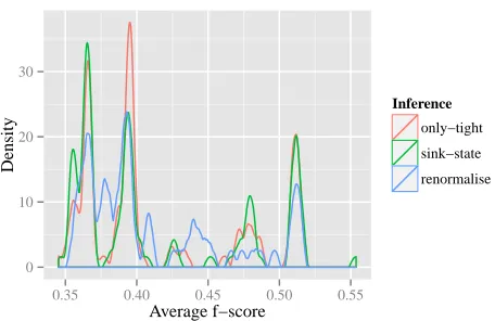
Figure 1: The density of theF1-scores with the three

ap-proaches. The prior used is a symmetric Dirichlet with α= 0.1.

P(ti|w) =

q(ti)

P3

i0₌₁q(ti0)

where the q used is based on the approach to tightness desired. For the sink-element approach, P(t1|w) = ₁₁7 ≈ 0.636364. For the

only-tight approach P(t1|w) = 11179₁₇₂₂₁ ≈ 0.649149.

For the renormalization approach the analytic ex-pression is too complex to include in this pa-per, but it approximately equals 0.619893. A log of our Mathematica calculations is available

at http://www.cs.columbia.edu/˜scohen/

acl13tightness-mathematica.pdf, and we

confirmed these results to three decimal places using the samplers described above (which required 107 samples per approach).

While the differences between these conditional probabilites are not great, the conditional probabili-ties are clearly different, so the three approaches do in fact define different distributions over trees under a uniform prior on rule probabilities.

9 Empirical effects of the three approaches in unsupervised grammar induction

ferences in the estimates produced by the three dif-ferent approaches to tightness just described. The bottom line of our experiments is that we could not detect any significant difference in the estimates produced by samplers for these three different ap-proaches.

In our experiments we used the English Penn tree-bank (Marcus et al., 1993). We use the part-of-speech tag sequences of sentences shorter than 11 words in sections 2–21. The grammar we use is the PCFG version of the dependency model with va-lence (Klein and Manning, 2004), as it appears in Smith (2006).

We used a symmetric Dirichlet prior with hyper-parameterα= 0.1. For each of the three approaches for handling tightness, we ran 100 times the sam-plers in§7, each for 1,000 iterations. We discarded the first 900 sweeps of each run, and calculated the F1-scores of the sampled trees every 10th sweep

from the last 100 sweeps. For each run we calcu-lated the average F1-score over the 10 sweeps we

evaluated. We thus have 100 averageF1-scores for

each of the samplers.

Figure 1 plots the density ofF1scores (compared

to the gold standard) resulting from the Gibbs sam-pler, using all three approaches. The mean value for each of the approaches is0.41with standard devia-tion 0.06 (only-tight),0.41 with standard deviation 0.05(renormalization) and0.42with standard devi-ation0.06(sink element). In addition, the only-tight approach results in an average of 437 (s.d., 142) re-jected proposals in 1,000 samples, while the renor-malization approach results in an average of 232 (s.d., 114) rejected proposals in 1,000 samples. (It’s not surprising that the only-tight approach results in more rejections as it keeps proposing new Θ until a tight proposal is found, while the renormalization approach simply uses the oldΘ).

We performed two-sample Kolmogorov-Smirnov tests (which are non-parametric tests designed to de-termine if two distributions are different; see DeG-root, 1991) on each of the three pairs of 100 F1

-scores. None of the tests were close to significant; the p-values were all above 0.5. Thus our experi-ments provided no evidence that the samplers pro-duced different distributions over trees, although it’s reasonable to expect that these distributions do in-deed differ.

In terms of running time, our implementation of the renormalization approach was several times slower than our implementations of the other two approaches because we used the naive fixed-point al-gorithm to compute the partition function: perhaps this could be improved using one of the more so-phisticated partition function algorithms described in Nederhof and Satta (2008).

10 Conclusion

In this paper we characterized the notion of an al-most everywhere tight grammar in the Bayesian set-ting and showed it holds for linear CFGs. For non-linear CFGs, we described three different ap-proaches to handle non-tightness. The “only-tight” approach restricts attention to tight PCFGs, and per-haps surprisingly, we showed that conjugacy still ob-tains when the domain of a product of Dirichlets prior is restricted to the subset of tight grammars. The renormalization approach involves renormaliz-ing the PCFG measureµover trees when the gram-mar is non-tight, which destroys conjugacy with a product of Dirichlets prior. Perhaps most surpris-ingly of all, the sink-element approach, which as-signs the missing mass in non-tight PCFG to a sink element ⊥, turns out to be equivalent to existing practice where tightness is ignored.

We studied the posterior distributions over trees induced by the three approaches under a uniform prior for a simple grammar and showed that they dif-fer. We leave for future work the important question of whether the classes of distributions over distribu-tions over trees that the three approaches define are the same or different.

We described samplers for the supervised and un-supervised settings for each of these approaches, and applied them to an unsupervised grammar induction problem. (The code for the unsupervised samplers is available from http://web.science.mq.edu. au/˜mjohnson).

Acknowledgements

We thank the anonymous reviewers and Giorgio Satta for their valuable comments. Shay Cohen was supported by the National Science Foundation under Grant #1136996 to the Computing Research Associ-ation for the CIFellows Project, and Mark Johnson was supported by the Australian Research Council’s Discovery Projects funding scheme (project num-bers DP110102506 and DP110102593).

References

K. B. Atherya and P. E. Ney. 1972. Branching Processes. Dover Publications.

Y. Bar-Hillel, M. Perles, and E. Shamir. 1964. On for-mal properties of simple phrase structure grammars.

Language and Information: Selected Essays on Their Theory and Application, pages 116–150.

T. L. Booth and R. A. Thompson. 1973. Applying prob-ability measures to abstract languages.IEEE Transac-tions on Computers, C-22:442–450.

Z. Chi and S. Geman. 1998. Estimation of probabilis-tic context-free grammars. Computational Linguistics, 24(2):299–305.

Z. Chi. 1999. Statistical properties of probabilistic context-free grammars. Computational Linguistics, 25(1):131–160.

S. B. Cohen and N. A. Smith. 2012. Empirical risk min-imization for probabilistic grammars: Sample com-plexity and hardness of learning. Computational Lin-guistics, 38(3):479–526.

M. H. DeGroot. 1991. Probability and Statistics (3rd edition). Addison-Wesley.

M. Johnson, T. L. Griffiths, and S. Goldwater. 2007. Bayesian inference for PCFGs via Markov chain Monte Carlo. InProceedings of NAACL.

D. Klein and C. D. Manning. 2004. Corpus-based induc-tion of syntactic structure: Models of dependency and constituency. InProceedings of ACL.

K. Kurihara and T. Sato. 2006. Variational Bayesian grammar induction for natural language. In8th Inter-national Colloquium on Grammatical Inference. K. Lari and S.J. Young. 1990. The estimation of

Stochas-tic Context-Free Grammars using the Inside-Outside algorithm. Computer Speech and Language, 4(35-56). M. P. Marcus, B. Santorini, and M. A. Marcinkiewicz. 1993. Building a large annotated corpus of En-glish: The Penn treebank. Computational Linguistics, 19:313–330.

M.-J. Nederhof and G. Satta. 2008. Computing parti-tion funcparti-tions of PCFGs. Research on Language and Computation, 6(2):139–162.

C. P. Robert and G. Casella. 2004. Monte Carlo Statisti-cal Methods. Springer-Verlag New York.

N. A. Smith. 2006.Novel Estimation Methods for Unsu-pervised Discovery of Latent Structure in Natural Lan-guage Text. Ph.D. thesis, Johns Hopkins University. C. S. Wetherell. 1980. Probabilistic languages: A