Design and analysis of strut based lattice structures for vibration isolation

Contents lists available atScienceDirect

Precision Engineering

journal homepage:www.elsevier.com/locate/precision

Design and analysis of strut-based lattice structures for vibration isolation

Wahyudin P. Syam

, Wu Jianwei

, Bo Zhao

, Ian Maskery

, Waiel Elmadih

, Richard Leach

a_{Manufacturing Metrology Team, Faculty of Engineering, University of Nottingham, NG7 2RD, UK}

b_{Ultra-Precision Optoelectronic Instrumentation Engineering Center, Harbin Institute of Technology, 150001, China} c_{Centre for Additive Manufacturing, Faculty of Engineering, University of Nottingham, NG7 2RD, UK}

A R T I C L E I N F O

Keywords:

Additive manufacturing Design

Lattice structures Vibration isolation Natural frequency

A B S T R A C T

This paper presents the design, analysis and experimental verification of strut-based lattice structures to enhance the mechanical vibration isolation properties of a machine frame, whilst also conserving its structural integrity. In addition, design parameters that correlate lattices, withfixed volume and similar material, to natural fre-quency and structural integrity are also presented. To achieve high efficiency of vibration isolation and to conserve the structural integrity, a trade-offneeds to be made between the frame’s natural frequency and its compressive strength. The total area moment of inertia and the mass (atfixed volume and with similar material) are proposed design parameters to compare and select the lattice structures; these parameters are computa-tionally efficient and straight-forward to compute, as opposed to the use offinite element modelling to estimate both natural frequency and compressive strength. However, to validate the design parameters,finite element modelling has been used to determine the theoretical static and dynamic mechanical properties of the lattice structures. The lattices have been fabricated by laser powder bed fusion and experimentally tested to compare their static and dynamic properties to the theoretical model. Correlations between the proposed design para-meters, and the natural frequency and strength of the lattices are presented.

1. Introduction

Additive manufacturing (AM) allows almost infinite geometrical design freedom [1], and the range and mix of potential materials is increasing [2,3]. However, despite the benefits afforded with having such freedom in design, there is a correspondingly larger design space that can be difficult to navigate. In this paper, we demonstrate how relatively simple design parameters can be used to reduce the design space and pinpoint a near-optimum design.

AM lattices are popular because they exhibit various advantages over solid stuctures and non-additively manufactured cellular solids. AM lattices have all the advantages of cellular solids, for example, low-mass and high impact energy absorbtion, and have an additional ad-vantage: a high degree of design freedom. The freedom to exploit lattice designs is a big advantage that enables, for example, the design of lattices with material grading to provide variations in their structural properties and a controllable deformation property to avoid undesirable failure modes[4]. Another advantage of the freedom of lattice design is that topologically optimised solutions to various problems, for example mechanical, thermal, vibration and energy absorption, can be im-plemented. In addition, AM lattices can provide better solutions to problems where the loading condition is unpredictable during

operation[4].

1.1. Design for AM to isolate vibration: motivation

This study presents design, experimental methodology and design parameters focusing on how to select a lattice design from many fea-sible strut-based lattice designs, within the same volume and from one material, to be used for a high-efficiency vibration isolation structure and to have sufficient structural integrity to sustain a mass load. Potential applications include metrology frames, machine frames and mounting brackets to support rotary components. Conventionally, to reduce the effect of vibration, both from the system itself and from the environment, stiffness structures are used, for example, a high-mass solid structure. However, the use of a solid structure does not isolate vibration transferred to the system, rather, the structure at-tenuates the vibration amplitude[5].

Vibration isolation is compared to vibration damping inFig. 1, which considers a simple case where vibration is transferred from an external vibration source to a machine. InFig. 1, the abscissa is the ratio r between the frequency of an external vibration f and the natural frequency of the machinefn. The ordinate is the displacement

ampli-tudedof the machine with respect to the displacement amplitude of the

http://dx.doi.org/10.1016/j.precisioneng.2017.09.010

Received 9 May 2017; Received in revised form 2 August 2017; Accepted 19 September 2017

⁎_{Corresponding authors.}

E-mail addresses:[email protected](W.P. Syam),[email protected](W. Jianwei).

0141-6359/ © 2017 The Authors. Published by Elsevier Inc. This is an open access article under the CC BY license (http://creativecommons.org/licenses/BY/4.0/).

external vibration source.C is damping coefficient that can be in the form of a different component or can be from the structure itself[5].

InFig. 1, vibration damping reduces the amplitude of the trans-ferred displacement due to the vibration. The machine is considered to become one structure with the external vibration source when the fraction of the transferred displacement to the part is equal to unity (see Fig. 1). When the ratio between the frequency of the vibration source and the natural frequency of the part is equal to unity, the amplitude of the part displacement will be amplified, having a significantly higher value than the original source displacement; this phenomenon is called resonance[5].

As an alternative to vibration damping, vibration isolation can be used to reduce the vibration amplitude transferred to the machine, with respect to the external vibration, by separating (isolating) the part from the external vibration source (see Fig. 1). Vibration isolation is more effective at reducing the effect of vibration compared to damping be-cause it does not require high mass (weight) to suppress the machine’s displacement due to the vibration and it can reduce the displacement of the machine to less than that of the external vibration. The higher the ratior, the more the part is isolated from the external vibration. To have a high value ofr,fnshould be smaller than f. A highrvalue can be

achieved by lowering the stiffness of a structure, but, there is a practical limit: if the stiffness is too low, the structure will be unable to sustain mass loads. InFig. 1,f_nis directly proportional to square root of stiff-ness over mass ( k m/ )[5].

1.2. Research aim

In this paper, design and analysis of several lattices and experi-mental methodology to verify the lattices’natural frequency and stiff -ness (mainly due to bending) are presented. In addition, design para-meters are proposed to allow comparison and selection of the optimum design for a strut-based lattice structure, from the potentially large number of feasible designs. All considered designs have the same vo-lume and are fabricated from the same material. The selection focuses on two properties: high-efficiency vibration isolation and sufficient structural integrity to be able to sustain specific mass loads. The design parameters should be able to capture the information about different lattice topologies (configurations) and can be correlated to the natural frequency of different lattices. To capture topology information, the total area moment of inertia of a strut-based lattice and its mass (at fixed volume) are proposed as design parameters.

In this study, because the strut material is identical for all the ex-amined lattice types, two hypotheses are proposed: (1) the stiffness of a lattice is proportional to its total area moment I m/ of inertiaI, and (2) the natural frequencyfnof a lattice is proportional to I/m. By using

I/m andIto representfnand the stiffness of a lattice, respectively, at

the design stage, a significant reduction in computational effort to comparefnand stiffness can be obtained, compared to multiple

ex-perimental tests or finite element analysis (FEA) procedures. FEA methods, commonly used to predict the natural frequency and com-pressive strength of a lattice structure, are computationally intensive and require specific procedures to be followed, such as convergence tests[4]. Moreover, the two hypotheses allow the selection of an op-timum lattice design from many feasible designs. For each of the lattice structures considered in this work, the stiffness is dominated by bending stress. This was determined by considering Maxwell’s criterion [7], which relates the deformation mechanism of a structure to its nodal connectivity

2. Lattice structure designs, analyses and simulations

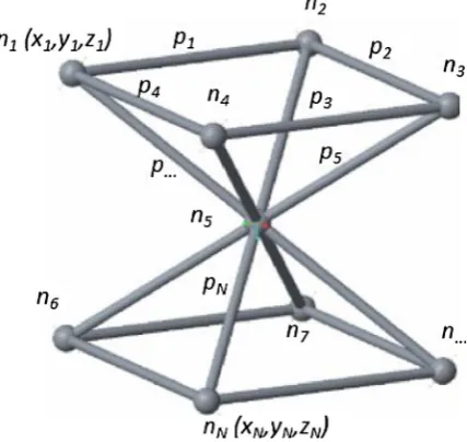
There are a large number of feasible options for designing strut-based lattice structures within a defined volume. A lattice structure consists of nodes (n) and struts (p), as illustrated inFig. 2. A node is a joint where two or more struts meet, and a strut is a link or member that connects two nodes. If the number of nodes and struts are not con-strained, then there will be a potentially large number of feasible strut-based lattice configurations that can be designed within afixed volume. The large number of options results from the variation of the number of Fig. 1.Graph illustrating vibration damping and isolation.

nodes and struts, the variation of node positions in a specific volume, the variation of node and strut diameters and multiple combinations of struts.

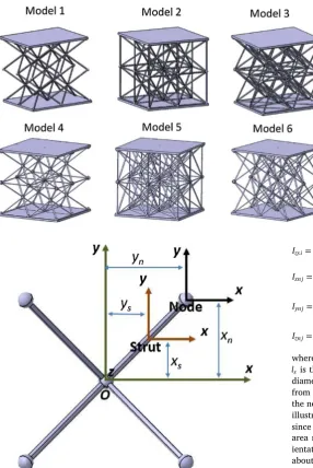
To demonstrate the use of the proposed design parameters and to reduce the design space, several lattice parameters have beenfixed. The fixed parameters are the number, positions and diameters of the nodes, and the diameter of the struts. Byfixing these parameters, the number of lattice design configurations can be significantly reduced. Six models of lattices based on configurations of nine nodes are presented, as shown inFig. 3. Model 1 is a body-centred-cubic (BCC) which is the simplest configuration of lattice cell with nine nodes[6]. The other models are generated by varying the strut configuration while main-taining the symmetry, allowing duplication in three directions, of the lattice designs. The number and combination of struts connecting two nodes are the diffierences among the six models. Each of the six single-cell lattice models, presented in Fig. 3, has a constant volume of (25 × 25 × 25) mm. Based on a common topology representation[7], the strut is represented as a cylinder with a diameter of 1.5 mm and the node is represented as a sphere with a diameter of 2 mm.

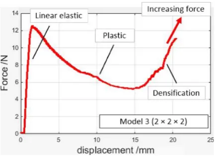
Lattice structures are rarely used in the form of a single unit[8], so they have been fabricated and experimentally verified in the form of a (2 × 2 × 2) unit cell configuration; this means every 2 × 2 × 2 con-figuration has eight identical lattice unit cells that shape a cubic sample. The 2 × 2 × 2 configuration is selected because it minimally represents a repeated form of lattices and shows the essential proper-tites of lattices (seeFig. 4). When a lattice is under compression, it undergoes three processes: elastic deformation, energy absorption (plateu region) and densification. The 2 × 2 × 2 configurations un-dergo the three processes under compression, as shown in Fig. 4, therefore, confirming they exhibit lattice behaviour. It is worth noting, in practice, lattice structures can be made with many more repeated forms than a 2 × 2 × 2 configuration. The 2 × 2 × 2 configurations are shown inFig. 5. By default, the bulk volume of each of the six lattice models in the configuration shown inFig. 5is (50 × 50 × 50) mm. In Fig. 5, 2 mm thickness plates are included into the designs. The purpose of adding the plate is to allow for the mounting of an accelerometer sensor for impact tests and to simulate a real situation where lattice structures are commonly designed as repeated structures between thin plates used as boundary walls[9].

2.1. Design parameter variables: total area moment of inertia and mass

Thefirst design parameter is the total area moment of inertiaI,

which is constituted byIx,IyandIzabout thex-,y- andz-axes

respec-tively. Therefore,Iis calculated as the summation ofI Iz x,Iyand

The calculations of the totalIx,IyandIzare carried out by summing

all individual areaIznmoments of inertia of each strutp:Ixs,IysandIzs

and each noden:Ixn,Iynand

The area total moments of inertiaIx,IyandIzare defined as:

∑

∑

= +

= =

Ix I I

i N

xs i j N

xn j

1 1

strut node

(1)

∑

∑

= +

= =

Iy I I

i N

ys i j N

yn j

1 1

strut node

(2)

∑

∑

= +

= =

Iz I I

i N

zs i j N

zn j

1 1

strut node

(3) whereIxs,IysandIzsare the area moments of inertia of strutspabout the x-,y- andz-axes, respectively,Ixn,Iyn andIzn are the area moments of

inertia of strutsn about to thex-,y- andz-axes, respectively,i is an index of theith_{strut and j is an index of thej}th_{node. The number of} nodes and struts are denoted asNnodeandNstrutrespectively (seeFig. 2).

The parallel axis theorem[10]is applied to calculate I for each strut:Ixs,IysandIzsand for each noden:Ixn,Iyn andIzn. Fig. 6is an

illustration of the parallel axis theorem from a two-dimensional (x- and y-planes) perspective. InFig. 6, the moments of inertia for each strutp

Fig. 3.Six models of lattice unit cells.

and for each noden can be calculated with respect to a central co-ordinate systemIx,Iy andIzfor thex-,y- andz-axes. The central

co-ordinate system (the originO) is calculated as the centroid of all the node coordinates. Hence, the moments of inertia for each strut and node are calculated as:

= +

Ixs i Ix's i l d xs s s2 (4)

= +

Iys i Iy's i l d ys s s2 (5)

= +

Izs i IZ's i l d zs s s2 (6)

= +

I I πd x

4

xn j xn n n

2 2

(7)

= +

I I πd y

4

yn j yn n n

2 2

(8)

= +

I I πd z

4

zn j zn n n

2 2

(9) whereiandjare the index for theith_{strut and then}th_{node respectively,} lsis the length of the strut,dsis the diameter of the strutp,dnis the

diameter of noden,xs,ysandzsare the distances of the strut’s centroid

from the originOalong each axis, andxn,ynandznare the distances of

the node’s centroid from the originO(seeFig. 6for a two-dimensional illustration in thexy-plane). In Eqs.(7)–(9), the indexesiandjvanish, since all the nodes and struts are the same size.Ix's i,Iy's iandIZ

'

s iare the area moment of inertia of thei-th strut when it is in a horizontal or-ientation.Ixn,Iyn andIzn are the area moment of inertia of the node

about thex-,y- andz-axes respectively. Since the node is a spherical shape which has the same form in any orientation,Ixn,IynandIzn are

equal and can be defined as follows[10]:

= = =

( )

I I I

π

4 .

xn yn zn

d 2

4

n

(10) To calculateI_x'_{s i},I_y'_{s i}andI_Z'_{s i}, a transformation of the axes to which the area moment of inertia refers should be carried out, since not every strut is parallel (horizontal) with respect to the central axesO. The derivation of the transformed axes to calculate Ix's i, Iy's i and IZ

'

s i, is shown inFig. 7, illustrated only forIx's iandIy's iin a two-dimensionalxy -plane. The derivation is shown for Ix's i andIy's i only, because the

Fig. 5.Representation of the 2 × 2 × 2 configuration for each of the six lattice models, each model having eight identical lattice unit cells.

Fig. 6.Variables used Ixs, Iys, Ixnand Iynfor each strut p and n in a 2D xy-plane view.

calculations forIZ's iis similar to the calculation ofIy i's. FromFig. 7, the distances of the elements of the struts (shown with a blue square in Fig. 7) x′andy′to the rotatedx- andy-axes, respectively, can be de-fined as:

′ = +

x xcosθ ysinθ (11)

′ = −

y ycosθ xsinθ (12)

whereθis the degree of rotation of the strut from the origin. From the basic definition of area moment of inertiaIof a solid body, IxsandIysare defined in[10].Ixs andIysareI of a rectangular

cross-section area, since the strut’s cross-sectional area along its long direc-tion is a rectangular area. By inserting equadirec-tion (11) into the basic formula forIxs[10], we can obtain for eachi-th strut:

= − +

Ix i's [cos ]θi2Ixs 2 sinθicosθ Ii xys [sin ]θi2Iys (13) whereIxysis a product of inertia and is equal to zero since the strut has a symmetrical cross-section area[12]. Hence,Ix's i becomes:

= +

Ix's i [cos ]θi2Ixs [sin ]θi2Iys (14)

= +

I [cos ]θ d l θ d l

12 [sin ] 12.

x i

s s

i s s

' 2 3 2 3

s i ₍₁₅₎

By substituting Eq. (12) into the basic formula for Iys [10]and

calculating in a similar way as in equations(13)–(15),Iy's ifor eachi-th strut becomes:

= +

I [cos ]θ d l θ d l

12 [sin ] 12 .

y' i2 s s i s s

3

2 3

s i ₍₁₆₎

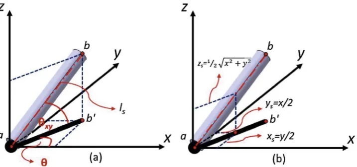
The calculation forIZ's ifor eachi-th strut is similar to the calculation ofIy's iand can be calculated as (seeFig. 8):

= +

I [cosθ ] d l θ d l

12 [sin ] 12

Z' xy i2 s s xy i s s

3

2 3

i ₍₁₇₎

whereθxyis the rotation angle of the strut with respect to planexy. The

calculations forIxs_i,Iys_iandIzs_iare summarised as follows (based on

Fig. 8):

= + +

I [cos ]θ d l θ d l l d x

12 [sin ] 12

xs i i2 s s i s s s s s

3 2 3 ' 2 (18) = + +

I [cos ]θ d l θ d l l d y

12 [sin ]

( ) 12

ys i i2 s s i s s s s s

3 2 ' 3 2 (19) = + +

I [cosθ ] d l θ d l l d z

12 [sin ] 12

zs i xy i2 s s xy i s s s s s

3

2 3

2

(20) where_x = = +

s y2 (y2 y1)2, ys=x2=(x2+x1)2, zs=12 x2+y2,

= +

ls' x2 y2,lsis the length of the strut,cosθxyis the inclination of the

strut with respect toz-axis,x=x2−x1, andy=y2−y1. Finally,Ifor the

two thin plates can be calculated in a similar wat to the calculation ofI

for the nodes. Instead, theIof the thin plates follows a rectangular cross-sectional area[10].

To calculate mass, it is straightforward to calculate the total volume of the struts (as cylinders) and nodes (as spheres) and multiplying by the material density. In this study, the material used to fabricate the lattices is Nylon-12 with densityρ= 1010 kg/m3_{.Table 2(row 1 and} row 2) shows the calculated total area moment of inertiaIand the mass for each of the six models in the 2 × 2 × 2 configuration inFig. 5.

2.2. Analysis of axial stress of each strut member in a lattice structure due to compressive stress

In this section, an FEA method to predict the ability of the lattice structures to sustain a load (structural integrity) is presented. To predict the structural integrity, a stiffness matrix method is used.

To analyse the structural integrity of the six lattice models, axial stresses on each strut are calculated and analysed. To predict whether the strength of a lattice structure is able to sustain a vertical load, all axial stresses on each strut should be less than the yield strengthYsof

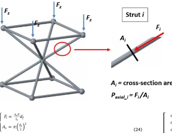
the lattice material. If there is more than one strut that has axial stress more than its yield strength, then the structure may fail to sustain the load. InFig. 9, an axial stress for eachith_{strut is denoted asP}

axial i. The

axial stressPaxial iis formulated as:

=

P F

A

axial i i

i (21)

whereFiis the axial force for theithstrutpandAiis the cross-section

area of the strut perpendicular to theFidirection.

A stiffness-matrix method is used to calculatePaxial ifor each node [11]. The method is then derived and extended to a 3D case and applied with MATLAB. Firtly, the method maps all the nodes and struts of a lattice into a symmetric global stiffness matrix. The second step is to calculate displacements for each strut p from a global displacement matrix. When the global stiffness and the displacement matrices are constructed, the axial force for each strutpcan be calculated by:

= D

Faxial K (22)

whereFaxialis aNdof×1matrix containingFion each strutpin thex,y

andzdirections.Kis aNdof×Ndof global stiffness matrix for each strut,

andDis aNdof×1global displacement matrix on each nodenin thex-, y- andz-directions. BothKandDare based on the lattice global (origin) coordinate O(seeFig. 6).Ndof is the degree of freedom (dof) of the

lattice being analysed and is defined as:

= ×

Ndof Nnode 3. (23)

TheNdof is multiplied by three because 3D spatial coordinates are

being used. FromFig. 10a, the axial forceFican be calculated as: Fig. 8.Illustration of the calculation of I for a strut. (a) Illustration ofθandθxyand, (b) illustration of

⎧ ⎨ ⎩ = =

( )

i A E_l f

s d₂

2

s s

s

(24) whereEis Young’s modulus,df is the axial displacement andAsis the

cross-sectional area of the strut perpendicular toFi.

The global stiffness matrixKand the global displacement matrixD

have to be constructed from a stiffness matrix K′and displacement matrixD', repectively, with respect to the local coordinates of each strut and with respect to the origin. The stiffness matrix for each strutK'can be calculated as (seeFig. 10a):

′ = ⎡ ⎣ ⎢ − − ⎤ ⎦ ⎥ A E l

K 1 1

1 1 .

s

s (25)

The matrixK'is multiplied by a 2 × 2 matrix⎡ ⎣ ⎢ − − ⎤ ⎦ ⎥ 1 1

1 1 because each

strut only has two edges (the two ends of a strut). Moreover, the dis-placement matrixD'for all the struts can be defined as (seeFig. 10b):

⎡

⎣

⎢

⎢

⎢

⎢

⎢

⎢

⎢

⎢

⎢

⎢

⎢

⎢

⎢

⎢

⎤

⎦

⎥

⎥

⎥

⎥

⎥

⎥

⎥

⎥

⎥

⎥

⎥

⎥

⎥

⎥

D ' .

f f f f origin f origin f fn fny fnz fn fn fn 1 1 1 1 1 1 x y z x y origin z x origin z origin z

origin z ₍₂₆₎

It is worth noting that, similar toK', the matrixD'only has two nodes:f_iandf_{i origin}(Fig. 10b).K'andD'are calculated with respect to the local coordinates of each strut (Fig. 10a). SinceKandDare the global stiffness and displacement matrices, respectively, the displace-ment and stiffness for each strut in its local coordinates should be transformed to global coordinates.Fig. 10b shows how to transform from the strut local coordinates to the lattice global coordinates. To transform the local displacement and stiffness matrices to the global coordinates, a transformation matrixTshould be used, whereTis de-fined as:

Fig. 9.Illustration of stresses for each strut p.

= ⎡ ⎣ ⎢ … …… … …… ⎤ ⎦ ⎥

λ λ λ

λ λ λ

λ λ λ

λ λ λ

T

0 0 0

0 0 0

0 0 0

0 0 0

x y z

x y z

nx nx nx

nx nx nx

1 1 1

1 1 1 ₍₂₇₎

whereλx,λyandλzare the transformation multiplier with respect to

the x, y andz global coordinates respectively.λx, λy andλz are

cal-culated as:

= = −

= −

− +

(

)

λ θ x x

l

x x

x x y y z z

cos ( ) ( ) , x x F F s F F

F F 2 F F F F

2

2

i origin

i origin

i origin i origin i origin ₍₂₈₎

= = − = − − +

(

)

x x y y z z

cos ( ) ( ) , y y F F s F F

F F 2 F F F F

2

2

i origin

i origin

i origin i origin i origin ₍₂₉₎

= = −

= −

− +

(

)

λ θ z z

l

z z

x x y y z z

cos ( ) ( ) . z z F F s F F

F F 2 F F F F

2

2

i origin

i origin

i origin i origin i origin ₍₃₀₎

Hence, the globalKandDmatrices can be calculated as: =

K T K'TT ₍₃₁₎

and

=TD

D '. (32)

Finally, by substituting Eqs.(31)and(32) into Eq.(22), theFaxial

matrix can be calculated as:

Faxial=TTK′T TD′ (33)

By calculating the matricesFaxial andD, all axial forces and

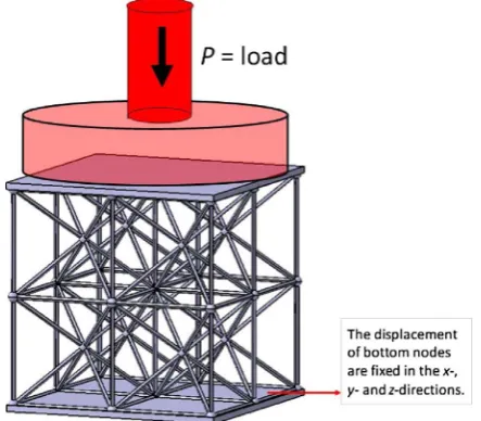
dis-placements (in the 3D spatial directions) of each strut can be obtained. To carry out the analyses, the material properties of the lattice structures and the boundary conditions for the analysis have to be de-fined. Nylon-12 is used as the material for lattice fabrication and test. The properties of Nylon-12 used in this study are obtained from the report by Ngim et al.[12]. The boundary conditions that are set for the truss analysis are: (1) the lower nodes of the six lattice models arefixed by setting their displacements in thex-,y-andz-directions to zero, and (2) the loads are applied vertically to each node at the top.Fig. 11

shows the boundary conditions to analyse the six lattice structures with the truss-matrix analysis. The total load selected for the polymer-based lattices is 5 N by considering small direct-current motors that com-monly have massses≤0.5 kg. The loads are distributed evenly across the upper nodes of the structures for numerical calculations.

From the structural analysis and after applying a 5 N total load, the maximum axial stress on each strut of the six lattices is compared to Nylon-12’s material yield strengthYs[12].Ysfor Nylon-12 is 0.054 GPa.

Results from the truss-matrix analysis revealed that lattice model 1, model 4 and model 6 have maximum axial stresses, among all the struts, that are greater thanYs. This result suggest that lattice model 1,

model 4 and model 6 cannot sustain the given compressive load. Lattice model 2, model 3 and model 5 show maximum axial stresses that are less thanYs, and can sustain the given load and satisfy the structural

integrity criteria.Table 2(row 6 and row 7) shows the maximum axial stresses for the six lattice models and the ability to sustain the load.

2.3. FEA simulation to estimate stiffness and natural frequency of the lattice structures

A commercial FEA software package ANSYS was used to simulate and estimate the stiffness and natural frequency f_n of the six lattice structures. Before starting the FEA analysis, a convergence test to de-termine the size of mesh elements, that controls the number of ele-ments, was carried out. The test was carried out by increasing the number of elements until the simulation output converges.

The convergence tests use model 1 and model 5 since they are the models with minimum and maximum strut elements, respectively. The test is carried out by increasing the number of elements (by decreasing the element size) until the difference of a result with respect to the previous result converges.Fig. 12shows the results of the convergence tests.

From the convergence tests, the number of mesh elements where the FEA results converge is around 95 000 elements for model 1 and around 220,000 elements for model 5 that correspond to element size of (0.4 × 0.4 × 0.4) mm. Hence, the mesh parameters used for the si-mulations are a quadrilateral element with a size of (0.4 × 0.4 × 0.4) mm. With the selected element size, the number of mesh elements for the 2 × 2 × 2 cubic lattice samples was around 95,000–220,000 ele-ments. Material properties used in this FEA are obtained from reference [12].

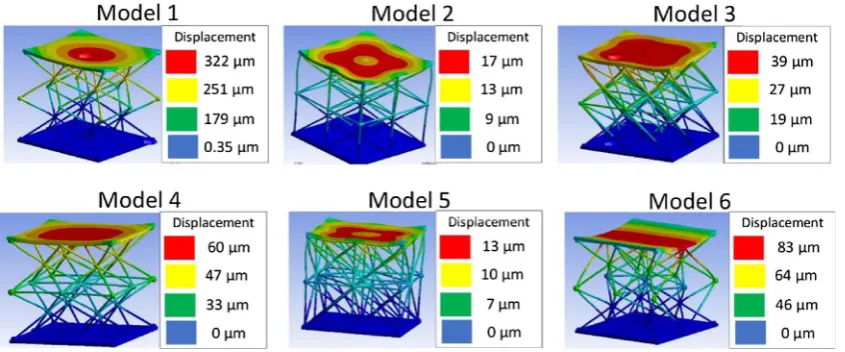
For the stiffness predictions for the lattices, an evenly distributed 1 N compression force is applied vertically on the top plate. The stiff-ness is calculated by dividing the compression force over the resulted displacement since the stiffness-displacement relation is still linear for a small force. The simulated stiffness is presented inTable 2(row 5). The force and boundary conditions are presented inFig. 11.Fig. 13shows results of the displacement of the six lattice models. FromTable 2, we can observe that lattice model 1 is the weakest structure among the six models.

The estimated f_nfor the lattice structures is presented in Table 2 (row 4). InTable 2, the simulatedf_nof the lattice models considers the first mode of vibration because this is the most dominant mode that occurs with oscillation along a vertical direction[5].Fig. 14shows the FEA simulation to estimate the f_nof mode 1 for all the lattice models. Results from the FEA inTable 2shows that thef_nof lattice model 5 is the highest and has the highest stiffness.

3. Experimental verification

3.1. Fabrication

For efficiency, only three lattice models were fabricated for ex-perimental verification; those were lattice model 1, model 2 and model 3. The reason to select the three lattices is as follows: (1) lattice model 1 has the least number of struts, (2) lattice model 2 and model 3 have Fig. 11.A set of boundary conditions and loads for the analysis of the axial stress for each

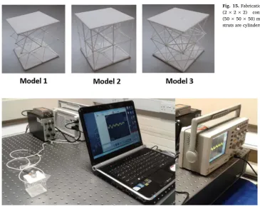
different behaviour, compared to the other lattice models, for their stiffness (seeTable 2row 1 and row 5), and (3) lattice model 3 has a larger area moment of inertia than model 2, but a lower stiffness. The different behaviour could be related to lower bending stress in model 2. To carry out experimental tests to verify the predicted natural fre-quency f_n and compressive strengths of the selected three lattice models, the lattices were fabricated by means of a laser powder bed fusion (LPBF) process. The lattice structures were fabricated from Nylon-12 powder. Table 3shows the mechanical properties of selec-tively laser sintered Nylon-12. The results of the LPBF fabrication are shown inFig. 15.

3.2. Impact test

Impact tests were carried out to characterise the f_nvalues of the lattice structures[5]. The main components of the impact test are an accelerometer, a signal amplifier and an oscilloscope to read the

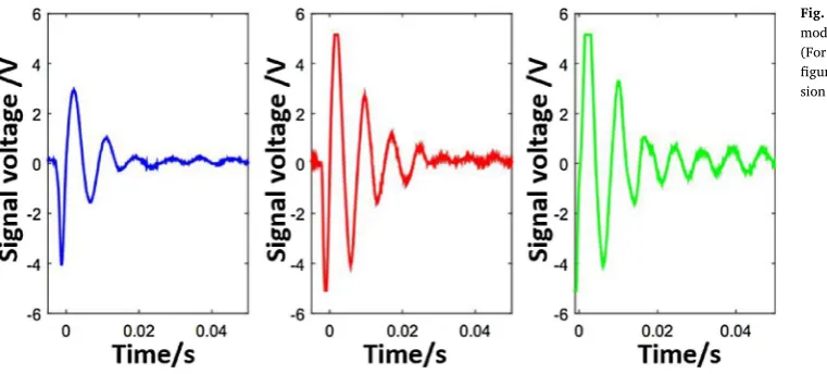
amplified signals from the accelerometer.Fig. 16shows the impact test experimental set up. The impacts are applied in the axial (vertical) direction. The calculated f_nvalues are the eigen mode 1 vibration os-cillation in the axial (vertical) direction.f_nvalues are calculated from the amplified signals read by the oscilloscope.Fig. 17shows samples of the recorded accelerometer signals due to vibration obtained by ap-plying an impact force to the lattice structures and recording the signals until they are completely attenuated.f_nvalues are calculated byfinding thefirst three consecutive peak points from the maxmum peak. The three points are then determined following common procedures[15].

For each lattice structure, both single cells and the 2 × 2 × 2 samples, three repeat measurements were carried out. In addition, the impact tests were carried out on two parts for each lattice model. The total number of impact tests was eighteen: three selected lattice models, three repeats for each model, and two fabricated parts for each model. Since thef_nestimation involved two parts for each model, the standard deviation of the mean of the calculatedf_nvalues is used to quantify the Fig. 12.Convergence tests to select the size of the elements in the meshing process. (a) Convergence tests for natural frequencyfn, and (b) convergence tests for displacement.

part-to-part variation. In addition, for comparison purposes, a solid cube model with size of (25 × 25 × 25) mm was fabricated with the same Nylon-12 material and also tested.

3.3. Compression tests

To test the compressive strength of the lattice models, compression tests were carried out by using a universal tensile test machine. The test was carried out by applying an axial compressive force with compres-sion speed 1 mm min−1. Fig. 18(left) shows the results of the com-pression tests for the selected three lattice models, andFig. 18(right) shows one of the compression tests. The compression speed was set to 1 mm min−1for all the tests. A total of nine compression tests were carried out (three selected lattice models with three compression tests for each model). InFig. 18(left), the displacement data are only shown up to the maximum force before plastic deformation occurs[8].

3.4. Results and discussion

From the results in Table 1, model 1 has the minimum natural frequency of 50 Hz, model 3 has 320 Hz and model 2 has the maximum natural frequency of 500 Hz. Meanwhile, the results from FEA for natural frequency estimation are presented inTable 2 (row 4). Per-centage differences between the FEA and the experimental results are 4%–14% (see below).

For more verification and comparison of the impact test results, a solid cube model was fabricated and tested. The f_nof the solid cube model obtained from the experiment is 5170 Hz ± 80 Hz and from the simulation is 5250 Hz, giving a 1.5% difference. It is worth noting that the standard error of the impact test results consider part-to-part var-iation becase the measurements were carried out for two different parts for each model.

Table 1(row 2) shows the results of the stiffness measurements. The Fig. 14.FEA simulations to estimatefnof the lattice structures in 2 × 2 × 2 cubic sample configuration. Colour bars show normalised eigenvalues of the relative amplitudes of motion

due to vibration[5].

Fig. 15.Fabrication results of the three lattice structures in samples of (2 × 2 × 2) configuration. The dimension of each sample is (50 × 50 × 50) mm. The nodes are spheres with 2 mm diameter and the struts are cylinders with 1.5 mm diameter.

results show that the maximum stiffness of 56,140 N m−1

is obtained for model 2, model 3 is 18,750 N m−1_{, while the minimum stiffness of} 3434 N m−1_{is obtained for model 1.}

The structural stiffnesses calculated from FEA are presented in Table 2(row 5). The percentage difference between the FEA and the experimental results of the stiffness ranges from 0.8% to 26%. Similar to the impact test results, the standard error of the results of the com-pression test consider part-to-part variation.

The uncertainty of the experiment results from both impact and compression tests are calculated as standard error of the mean. This type of uncertainty is called Type-A uncertainty[16]. Standard error is used to represent the precision of the calculated means from both the two tests[17]. The standard erroruis calculated as[17]:

=

u σ

n, (34)

whereσ is sample standard deviation andnis the number of repeat experiments. The values ofnfor the impact and compression tests are six and three, respectively.

The difference between the FEA and the experimental results for all the lattice models is most probably due to the nature of the LPBF process used to fabricate the lattices, the difference in the material properties between the FEA simulation and the fabricated lattices, and the geometrical discrepancies of the fabricated part from the nominal CAD models, for example, the size of the lattices’nodes and struts[13].

LPBF fabricates lattices that are not fully dense due to porosity defects, while the FEA simulation considered fully dense parts with ideal geo-metry.

To summarise (fromTable 1row 3), model 2 has the highest com-pressive strength having the maximum force, before plastic deformation occurs, of 19.25 N at 0.68 mm displacement. Model 1 has the minimum compression force that is 2.21 N with displacement at 1.62 mm. Model 3 has a compressive force higher than that of model 1 but lower than that of model 2. For model 3, the compressive force before plastic de-formation occurs at 12.78 N with a displacement of 1.13 mm. It is worth noting that, the compression force of lattice model 1 is less than 5 N; this suggests that lattice model 1 cannot sustain the applied load of 5 N since, in model 1, the plastic deformation occurs before the com-pressive force reaches 5 N.

Table 2shows the summary of all the results of the calculated design Fig. 17.Samples of accelerometer signal from lattice model 1 (blue), model 2 (red) and model 3 (green). (For interpretation of the references to color in this figure legend, the reader is referred to the web ver-sion of this article.)

Fig. 18.Compression force against displacement for the selected three 2 × 2 × 2 lattice models: theRed lineis for model 2, thegreen lineis for model 3, and theblue lineis for model 1 (left). The compression test applied to model 3 (right). (For interpretation of the references to colour in thisfigure legend, the reader is referred to the web version of this article.)

Table 1

Summary of lattice properties from experiments (u denotes standard error).

No. Results 2 × 2 × 2 samples configurations

Model 1 Model 2 Model 3

1 fn/Hz 50 ± 6 500 ± 26 320 ± 14

2 k/N m−1 3434 ± 208 56140 ± 580 18750 ± 212

parameters and the simulated lattice properties, that is I, mass, f_n, strength and the maximum axial stress on the lattices’struts. From all six lattice models, only model 3, model 4 and model 5 can satisfy the structural integrity criteria to be able to sustain the load. Of these three models, model 3 has the lowestf_n. From the experimental results of the impact tests and the compression tests, the proposed design parameters: Iandmare proportional to the natural frequency and the strength of the lattice.Figs. 19 and 20show the correlation of f_nwith respect to k m/ and the correlation of the proposed parameter I m/ with respect to f_n, respectively. For each graph inFigs. 19 and 20, a least-squared line isfitted to the simulation results and the experimental results are shown with error bars. Before the linear regression analyses were ap-plied to data points, normality tests of the data points were carried out.

From the normality tests, the variation of the data points follow normal distribution (with P−value=0.85). It suggests that the regression analyses are valid. The regression analyses are applied to six data points from the six lattice models. The six lattice models cover a range from the model with the least number of struts (model 1) to the model with the most number of struts (model 5). Withfixed nine number of nodes, the lattice design space is limited to those six models.

Fig. 19shows the correlation betweenf_nand k m/ . FromFig. 19, the coefficient of determination (goodness offit)R2_{value is 0.99. From} theR2_{value, the data points do not follow thefit perfectly as in the case} of solid cubes. This result suggests that lattice structure vibration characteristics are not exactly equal to those of solid structures. The complex nature of lattice structures may affect this equality, for ex-ample, due to bending of their members.

Fig. 20shows the correlation between f_n and the proposed para-meter I m/ . FromFig. 20, the proposed parameter I m/ show a linear correlation to f_n. The determination coefficient R2 _{value of thefit is} 0.81. Hence, thefitting covers 81% variation of the data. InFig. 20, from analysis of variance (ANOVA) test for the regression analyses, the I m/ term is statistically significant (P−value=0.01) while the con-stant term (the intercept) is not significant (P−value=0.5). From ANOVA test, it suggests that the parameter I m/ has significant posi-tive correlation with f_n. The proposed parameters could be useful to Table 2

Summary of calculated design parameters and the simulated lattice properties.

No. Results 2 × 2 × 2 samples configurations

Model 1 Model 2 Model 3 Model 4 Model 5 Model 6

1 TotalI/m4

× −

4.19 10 6 _2.01×10−3 _3.01×10−3 _1.31×10−3 _5.71×10−3 _1.07×10−4

2 Mass/kg _9.74×₁₀−3 _1.08×10−2 _1.11×10−2 _1.04×10−2 _1.17×10−2 _1.10×10−2

3 I

m/(m4kg−1)1/2 ×

−

2.01 10 2 _4.30×10−1 _5.19×10−1 _3.53×10−1 _6.97×10−1 _9.84×10−2

4 fn/Hz( ± 1%) 47.5 501.5 325 240.5 640.5 190

5 k/N m−1( ± 1%) 3090 55600 25300 16500 75700 11900

6 Maximum axial stress from all the struts Paxial_i/GPa 0.079 0.015 0.048 0.078 0.017 0.088

7 Is able to sustain the load? No Yes Yes No Yes No

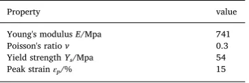
Table 3

Mechanical properties of LPBF Nylon-12 for uniaxial compres-sion[12].

Property value

Young's modulusE/Mpa 741

Poisson's ratiov 0.3

Yield strengthYs/Mpa 54

Peak strainεp/% 15

select a lattice configuration among many feasible options (at fixed volume and with one material) focusing on natural frequency and strength; the calculation of the parameter I andm are very efficient compared to FEA simulations or experiments to compare the f_n. Using the analytical model developed here the computing time for I m/ with an average desktop PC is generally seconds, while the computing time for k m/ by FEA, excluding the convergence test, is around 45 min with a high-performance computer.

FromFig. 20, model 2 has lowerIthan model 3, but model 2 has a higher stiffness than model 3. The reason can be traced to the stretch-dominated nature of model 2’s structure, and the bending-stretch-dominated nature of model 3’s structure. A stretch-dominated structure increases the strength of model 2 and a bending-dominated structure decreases the strength of model 3[7].

From the simulation and experimental results, it can be observed that lattice model 3 is a good compromise between f_nand the com-pression strength. Model 1, model 4 and model 6 have low f_nwhich is good for vibration isolation, but the structure of these three models cannot sustain the given load. Similar conclusions can be drawn for model 2 and model 5; the two lattice models have the highest com-pressive strength, but they also have the highest value of f_n.

The simulation and experiment results suggest that model 3 is the most suitable lattice structure to be selected out of the six lattice structure models proposed above for high-efficiency vibration isolation while fulfilling the structural integrity constraint. Model 3 has a suffi -cient strength but has a lower natural frequency compared to model 2 and model 5. A wide range of applications can utilise model 3 lattice design, for example, as a frame structure for a machine or as mounts for rotary equipment so that the vibration from the rotary equipment is isolated from the structure of interest considering an ideal situation where there is only one vibration source. For instance, a system related to rotational and linear motion typically has vibration generated from the motors, for example, a linear motor system can produce vibration with a frequency of more than 400 Hz[14].

Fig. 21illustrates the vibration isolation of lattice models 2–5 with an external vibration source oscillating at400Hz. Damping factorsζare

considered to be in a range from 0.2 to 0.5[18]. Damping factorζis a constant that directly proportional to damping coefficientC[5].Fig. 21 shows that lattice model 3 can reduce vibration more than lattice models 2 and 5 for all damping factors. Lattice models 1, 4 and 6 were not considered because they are too weak to sustain the predefined load, as can be seen inTable 2row 7. For the range of damping factors considered here, the maximum vibration reduction that lattice model 3 can provide is 26% atζ=0.5(the transferred amplitude is74%from the source amplitude), while models 2 and 5 do not reduce the vibration. Finally, the effectiveness of model 3 lattice structure to isolate vibra-tions also depends on the various vibration frequencies of the system of interest.

4. Conclusions and future work

The paper proposes design parameters to compare lattice designs considering the natural frequency and the compression strength, and to select a design that has high efficiency vibration isolation properties, that at the same time, is able to sustain loads. The proposed parameter is straightforward and efficient to calculate rather than to run FEA si-mulations, which are computationally extensive.

Future work includes, an investigation of a more comprehensive model to estimate natural frequency of lattice structures. The effect of bending of the members of a lattice structure is expected to contribute to its natural frequency. In addition, a full six degrees of freedom model of the vibration of lattices should be investigated.

The design parameters can be integrated into an iterative optimi-sation procedure as an objective function. With iterative procedures, a wider and more complex design space can be explored tofind a better strut-based model that has high vibration isolation efficiency for a system of interest.

Further work will study the various types of defects of fabricated lattice structures, for example, part porosity and geometry imperfec-tions, and their correlation to the degradation of mechanical perfor-mance properties, for example, natural frequency and compressive strength of the lattice structures.

Acknowledgements

The authors would like to thank EPSRC (grant: EP/M008983/1) for funding this work and Prof. T. L. Schmitz (UNC Charlotte, USA) and Dr Dimitrios Chronopoulos (The University of Nottingham, UK) for fruitful discussions.

References

[1] Thompson MK, Moroni G, Vanekar T, Fadel G, Campbell I, Gibson I, et al. Design for additive manufacturing: trends, opportunities, considerations and constraints. Ann CIRP 2016;65:737–60.

[2] Rosen DW. Research supporting principles for design for additive manufacturing. Virtual Phys Prototyp 2014;9:225–32.

[3] Gibson I, Rosen DW, Stucker B. Additive manufacturing technologies: rapid proto-typing to direct digital manufacturing. New York, USA: Springer; 2010. [4] Maskery I, Aboulkhair NT, Aremu AO, Tuck CJ, Ashcroft IA, Wildman RD, et al. A

mechanical property evaluation of graded density Al-Si10-Mg lattice structures manufactured by selective laser sintering. Mater Sci Eng A-Struct 2016;670:264–74. [5] Schmitz TL, Smith KS. Mechanical vibrations: modelling and measurement. New

York: Springer; 2012. p. 87.

[6] Maskery I, Hussey A, Panesar A, Aremu A, Tuck C, Ashcroft I, et al. An investigation into reinforced and functionally graded lattice structures. J Cell Plast

2017;53:151–65.

[7] Deshpande VS, Ashby MF, Fleck NA. Foam topology bending versus stretching dominated architectures. Acta Mater 2001;49:1035–40.

[8] Rashed MG, Ashraf M, Mines RAW, Hazell PJ. Metallic microlattice materials: a current state of the art on manufacturing, mechanical properties and applications. Mater Design 2016;95:518–33.

[9] Nguyen J, Park SI, Rosen D. Heuristic optimization method for cellular structure design of light weight components. Int J Precis Eng Manuf 2013;14:1071–8. [10] Gere GM, Timoshenko SP. Mechanic of material. 3rd ed. New York: Springer; 1991.

p. 250.

[11] Hibbeler RC. Structural analysis. 8th ed. New York: Prentice Hall; 2012. p. 539. [12] Ngim DB, Liu JS, Soar R. Design optimisation of consolidated granular-solid

polymer prismatic beam using metamorphic development. Int J Sol Struc 2009;46:726–40.

[13] Ahmadi S M, Yavari S A, Wauthle R, Pouran B, Schrooten J, Weinans H, et al. Additively manufactured open-cell porous biomaterials made from six different space-filling unit cells: the mechanical and morphological properties. Materials 2015;8:1871–96.

[14] Zhang L, Long Z, Cai J, Fang W. Design of a linear macro-micro actuation stage considering vibration isolation. Adv Mech Eng 2015;7:1–13.

[15] Bower A, Vlahovska P, Xu J. Introduction to dynamics and vibration. PhD: School of Engineering Brown University; 2016.

[16] BIPM JCGM 100 2008 Evaluation of measurement data–Guide to the expression of uncertainty in measurement (GUM).

[17] Montgomery DC, Runger GC. Applied statistics and probability for engineers. New York: John Wiley & Sons; 2003. p. 225.

[18] Geethamma VG, Asaletha R, Kalarikkal N, Thomas S. Vibration and sound damping in polymers. Resonance 2014;9:821–33.