A BAYESIAN APPROACH TO ANALYZING PHENOTYPE MICROARRAY DATA ENABLES ESTIMATION OF MICROBIAL
GROWTH PARAMETERS
Preprint of an article published in Journal of Bioinformatics and Computational Biology 2016 DOI: 10.1142/S0219720016500074
c
World Scientific Publishing Company
http://www.worldscientific.com/doi/abs/10.1142/S0219720016500074
MATTHIAS GERSTGRASSER
Department of Computer Science, University of Oxford, Parks Road, Oxford, OX1 3QD, UK
SARAH NICHOLLS
School of Biosciences, University of Nottingham, Sutton Bonington, Leicestershire, LE12 5RD, UK
MICHAEL STOUT
School of Biosciences, University of Nottingham, Sutton Bonington, Leicestershire, LE12 5RD, UK
KATHERINE SMART SAB Miller plc, Church Street West,
Woking, GU21 6HS, UK [email protected]
CHRIS POWELL
School of Biosciences, University of Nottingham, Sutton Bonington, Leicestershire, LE12 5RD, UK
THEODORE KYPRAIOS
School of Mathematics, University of Nottingham, Nottingham, NG7 2RD, UK
DOV STEKEL
Received (Day Month Year) Revised (Day Month Year) Accepted (Day Month Year)
Biolog phenotype microarrays enable simultaneous, high throughput analysis of cell cul-tures in different environments. The output is high-density time-course data showing redox curves (approximating growth) for each experimental condition. The software pro-vided with the Omnilog incubator/reader summarizes each time-course as a single da-tum, so most of the information is not used. However, the time courses can be extremely varied and often contain detailed qualitative (shape of curve) and quantitative (values of parameters) information. We present a novel, Bayesian approach to estimating pa-rameters from Phenotype Microarray data, fitting growth models using Markov Chain Monte Carlo methods to enable high throughput estimation of important information, including length of lag phase, maximal “growth” rate and maximum output. We find that the Baranyi model for microbial growth is useful for fitting Biolog data. More-over, we introduce a new growth model that allows for diauxic growth with a lag phase, which is particularly useful where Phenotype Microarrays have been applied to cells grown in complex mixtures of substrates, for example in industrial or biotechnological applications, such as worts in brewing. Our approach provides more useful information from Biolog data than existing, competing methods, and allows for valuable comparisons between data series and across different models.
Keywords: Biolog, Growth Model, Diauxic, Lag Phase, Bayesian Statistics, Phenotype Microarrays
1. Background
Biolog Phenotype Microarrays (PMs) are unique patented commercial products for assessment of cellular respiration of prokaryotic and eukaryotic cells in a wide range of conditions, including metabolism using different carbon, nitrogen, phosphorous and sulphur sources, as well as osmotic, pH, antimicrobial and metal ion stresses. The PMs work by the reduction of a colourless tetrazolium dye in the growth me-dia to a purple formazan by electrons from the NADH produced during cellular respiration?. For microbial PMs, 1920 different phenotypes per organism (including controls) can be assessed simultaneously by using the full set of 20 different 96 well plates. As the assays are performed for 24 hours or longer, the output is high den-sity time-course data for each well (growth condition), showing a measurement of the quantity of dye reduced. A typical experiment can contain as many as 450,000 data points, making the output especially suitable for mathematical and statistical modelling. The PM platform is flexible, allowing users to construct their own assays using plates, growth media and tetrazolium dyes. Thus they have proven extremely flexible in terms of the experiments that can be carried out with them ?. Among other uses, Biolog OmniLog PM technology can be used in research aimed at un-derstanding and controlling the performance of biotechnological processes, through analysis of microbial metabolism in conditions relevant to industrial fermentations ?,?.
However, while PM technology can generate vast amounts of information about
microbial growth in the form of time-series data, its usefulness is limited by a lack of robust, easy to use and flexible data analysis tools for such data. Often, the data (which in its raw form comprises up to several hundred data points) is being reduced to either a binary “growth / no-growth” distinction or, at best, a single datum, such as maximum signal reading, average signal height reading or area under curve (AUC) ?,?. Clearly, a lot of information is lost this way.
Biolog’s own software allows rudimentary data analysis mainly focused at di-rectly comparing two different strains grown on PM plate types. As detailed in Bochneret al.?- cf. Box 1 therein - this consists of plotting curves from two strains (generally a mutant and a control strain) against each other and highlighting dif-ferences above a certain threshold. This results in effectively a ternary distinction between either of the strains showing higher respiration or there being no significant difference between them. Alternatively the software can give a numerical output of the difference in respiration rates between the two strains compared, as used for instance in?.
0 10 20 30 40 50 60 70
100
150
200
250
300
350
Time / hours
Biolog Units
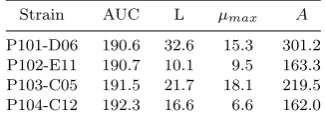
[image:4.595.160.422.203.450.2]P101−D06 P102−E11 P103−C05 P104−C12
Fig. 1. Respiration data taken from four different phenotypes in the datasets. Plot shows coloration (Biolog units) vs. time. All four curves have very similar AUC, yet it is clear that they are qualitatively different, with different lengths of lag phase and maximal growth rates.
Some previous research has been carried out in this area, but has been limited in its scope. For instance?focus on visualizing the raw Biolog data without any param-eter estimation. A more recent approach published in?provides both visualization as well as parameter estimation using the grofit R package. This package uses non-linear least squares regression to fit Gompertz and Richards models to growth curves, but also provides a model-free spline fit ?. The logistic growth model has also been found to be effective in fitting Biolog data and has been used to facilitate normalisation and data comparison?.
to assess the potential of PM technology in the differentiation of 100 proprietary brewing yeast strains in different worts. The focus of the paper is on the modelling and methodology and these data are brought as relevant examples.
We anticipate that these ideas have the potential to transform the capacity of research groups to obtain useful and meaningful information from Biolog Phenotype Array data.
2. Methods
2.1. Modeling aspects
A number of different growth models have been proposed in the literature?. These have different statistical properties?and it can be argued that their are limitations of the interpretations of these models ?. These models are generally derived in the form of an ordinary differential equation or as a system of ODEs, though many of them also have a closed-form expression. We will focus on two models in particular, described in the sections below. As the Biolog Omnilog PM machines measure respiration rather than growth, it is not a priori clear that any of the traditional growth models will be able to accurately fit the data produced in PM experiments. However, empirically we found that these models provide useful results.
2.2. The Baranyi model
We chose to focus mainly on the model developed by Baranyi and Roberts. This was first introduced in?, and discussed in more detail for instance in?,?. The model is based on the Richards model?, but introduces another inhibition term to model the lag phase. The inclusion of a lag phase is important, as growth and metabolism of microorganisms in fresh media typically results in an initial period of delayed activity. Consequently much of the data we analyzed includes a distinct lag phase; this can be seen in the example data shown in Figure ??. Thus models that do not include a lag phase (e.g. logistic growth), or models where there is insufficient flexibility over the shape and time of the lag phase (e.g. Gompertz models?) do not perform well. The form of the model we used is as in?:
d
dty=r·y·u(y)·α(t), (1)
whereα(t) accounts for the inhibition at the beginning of growth. For an isother-mal batch culture environment (e.g. as provided by Omnilog), the authors suggest setting
α(t) = q0
q0+ exp(−ν·t)
(2) Withu(y) as in the Richard’s model this gives a closed-form expression as fol-lows:
log(y(t)) = log(y0) +r·A(t)− 1
mlog
1 + e
mrA(t)−1
em(log(ymax)−log(y0))
where
A(t) = Z t
0
α(s)ds=t+ 1
ν log
e−νt+q0 1 +q0
(4)
In addition to the four parameters (y0, ymax, r, m) of the Richards model, this introduces another two parameters, ν and q0 that control the length and shape of the lag phase. This term is motivated biologically:q0 is to be taken as the initial physiological state of the cells, while ν gives the rate at which they adapt to their new environment. This gives the full Baranyi model a high degree of freedom in accommodating a wide range of growth curve data; as others have noted ? the Baranyi model performs very well in fitting empirical growth curve data.
There are two things we would like to point out. Firstly, the form ofα(t) makes it entirely independent of the rest of the Baranyi model. That is, it is straightforward to incorporate this lag term into other models, and we have done so for instance with a simple diauxic model which we discuss below. Secondly, for any given lag phase lengthλ, there is an infinite number of combinations ofq0andν that satisfy the formula for αgiven above. We have found it more convenient to parameterize the Baranyi model (and other models usingα(t)) withλandν rather thanq0 and
ν. We then deriveq0 by
q0= 1
eνλ−1 (5)
for use in the closed-form expression of the Baranyi model respectivelyα(t). In this form, one parameter controls the duration of the lag phase itself, whereas ν
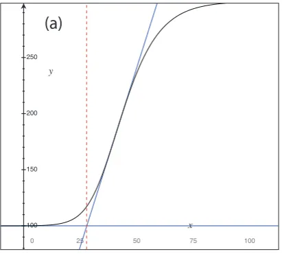
controls its shape. Figure ??(right) showsA(t) for a fixedλand varying values of
0 25 50 75 100
100 150 200 250
0 5 10 15
2.5 5 7.5 10
(a)
[image:7.595.213.419.214.399.2](b)
Fig. 2. Numerical derivation of a lag phase length from a Baranyi curve. (a) The calculated lag is 27.87 whereas the model lag parameter is 30. (Other model parameters:y0= 100, ymax= 300, r=
Baranyi suggested a slight simplification of the original model, setting m = 1 andν=r?. The resulting model is simpler than the original one and still fits most of the data we have seen; On the other hand, the original model is more flexible in fitting less typical growth curves. We thus adopted a two-fold strategy and used both the original and the simplified versions of the model, as well as two versions that incorporate either one of the proposed modifications.
2.3. Diauxic growth
As will be seen below, the example data we analyse (from worts), typical of growth on complex mixtures of substrates, includes curves that show a clear diauxic effect. We modeled this using a simple diauxic growth model based on Monod-type sub-strate inhibition terms. As a starting point we used the following model, in ODE form:
dy
dt =r1s1y+ k k+s1
r2s2y (6)
ds1
dt =−r1s1y, ds2
dt =−
k k+s1
r2s2y (7)
Whiles1 is large, this essentially gives logistic growth on substrate 1. As sub-strate 1 is being used up, the inhibition term k+sk
1 increases and logistic growth on substrate 2 starts. Smaller values of the inhibition constant kgive a more pro-nounced diauxic effect due to the stronger influence of s1 on the inhibition term.
k
k+s1 is a hyperbolic inhibition term that is supposed to model the inhibitory effects happening within the cells ass1 is being exhausted.
We amended this model to include a Baranyi-like lag phase term. In its non-integral form α(t) this transfers to our ODE model in a straightforward fashion, giving the following for our diauxic growth model:
dy dt =α(t)
r1s1y+
k k+s1
r2s2y
(8)
ds1
dt =−α(t)
r1s1y
,ds2
dt =−α(t)
k
k+s1
r2s2y
(9) Arguably, this model is a rather simplified view of the biological processes hap-pening but has empirically proven to be useful. A number of other models for diauxic growth have been proposed?,?. Our model is simpler (for example Kompalaet al.’s 1986 model has five parameters per substrate, ours has eight in total), but still sufficiently flexible to be able to describe virtually all of the diauxic growth curves we have seen.
2.4. Gompertz model
2.5. Parameter estimation
We adopted a Bayesian approach? to infer model parameters from the time-series data recorded by Biolog machines. In particular we used a variant of the Metropolis-Hastings algorithm? to sample from the posterior distribution of these parameters. This algorithm starts with an initial state vectorθ(0). At each iteration a candidate state vector θ0 is generated by drawing from a proposal distribution q(.|θi). With probability α(θi, θ0) that move is accepted, where
α(θi, θ0) = min 1,
p(θ0)q(θi|θ0)
p(θi)q(θ0|θi)
(10) If accepted, we setθi+1=θ0, otherwise setθi+1=θi. Theθi form a Markov chain, and the stationary distribution of this chain is the desired posterior distribution
p(θ) irrespective of the proposal distributionq(.|.)?or ?.
A number of modifications and amendments to the original Metropolis-Hastings algorithm have been proposed to better explore the target distribution or to im-prove the algorithm’s rate of convergence. In particular, significant attention has been drawn to the construction of adaptive algorithms, i.e. algorithms which do not require the specification of the tuning variance of the proposal distribution
q(.|.). One of the most commonly used algorithms is the Adaptive Metropolis (AM) algorithm? that has been discussed in detail in the literature?,?,?,?.
The use of an adaptive algorithm is important for the analysis of high throughput PM data because of the large number of data sets being analysed. Each PM plate contains 96 wells, and with an experiment of 100 plates this leads to 9,600 separate curves. It is not possible to manually tune the parameters for each curve so an automated, adaptive approach is necessary. We implemented an AM algorithm with global scaling as described in algorithm 4 in Andrieu and Thoms 2008 as follows:? (1) For an initial segment of the chain (i < i0, for some sensible choice of i0)
per-form a “Random-Walk Metropolis with global scaling” with proposal covariance matrixλiΣ0, with Σ0an initial “best guess” of the true covariance matrix. (2) For the remainder of the chain, do as above but use λiΣi as the covariance
matrix for the proposal distribution, where Σiis the sample covariance matrix of the previous history of the chain, and λi is a varying scaling factor. We update Σi iteratively.
We usedi0= 2500 (chosen empirically). For i < i0 we updated Σi andλi only when we accept a move, as suggested in Haario et al., 2001. ? We reset λ
i to its original value of 2.42/dim(θ) in iterationi
We used uninformative or uniform priors on suitable regions, and utilized sim-ple heuristics to give rough estimates of the initial parameter vector for the AM algorithm (See Appendix for details). These heuristics proved to be effective in that all Markov chains converged to a stationary distribution (see subsection on Per-formance below) after appropriate burn-in. Alternative approaches could be to use an iterative least-squares approach to obtain initial parameter values near to the stationary distribution?. To calculate the likelihood function, we assumed normally i.i.d. measurement errors, which we heuristically estimated from the raw data as detailed in the appendix.
2.6. Model choice
In addition to inferring parameters from them, we used the Deviance Information Criterion?,?. This is defined as follows:
DIC= ¯D+pV (11)
whereD is the deviance defined by
D(θ) =−2 log(p(x|θ)) (12) and ¯Dis the mean of this deviance. The model complexitypV is given aspV = var(D)/2. An alternate definition of DIC usespD= ¯D−D(¯θ) to account for model complexity. We have found however that this is highly dependent on the quality of the estimation of the posterior. In some cases where our posterior sample was not a good estimate, we saw thepD term dropping to artificially low (often negative) values leading to a bad, artificially low estimate of DIC. While it is possible to check that the posterior sample is reasonable before calculating DIC this way, we expect that in any high-throughput environment there will be individual data that slip through such checks. Thus we have found that using pV was in practice more suitable for our purposes. For comparison purposes we have also calculated BIC for all models?, using the highest likelihood observed in the posterior sample for the BIC estimate.
We used the DIC to choose which model to use to derive estimated parameters for each well. Furthermore, we were looking to get an indication as to whether our models provide a reasonable fit at all. To this end we compared them to a simple “dummy” model defined by y(t) = c for a constant parameter c. This is non-informative, and similar to a classicalH0model. A comparison via DIC or BIC to the constant model is meant to show whether the model fits the data at all.
2.7. Parameter comparisons between models
fitted curves. This is to allow for simple quantitative comparisons between wells that show qualitatively different behaviour.
In the following paragraphs we will takey(t;θ) to mean the signal level predicted by our model and the parameter vector θ at time t. Firstly, for A, the maximum coloration change achieved, we simply usedy(tlast;θ)−y(0;θ), that is, the absolute increase in coloration our model predicts over the period of time that was recorded in the experiment. It may be argued that for all the models we are using we could also compute a similarAfrom they0andymax(respectivelyy0ands1,s2). However, we found that if the recorded respiration data stops before a maximum is attained, the maximum or substrate level parameters are effectively inestimable, and so wouldA
be with such a definition. Note that if a maximum is effectively reached within the experiment record, these two definitions will for practical purposes be equivalent.
For µmax we took the steepest slope of y(t;θ) (again within the experiment period), as derived numerically from the fitted curve. This is not a transformation of the model’s rate parameter(s) alone, but is model-independent and coincides with a more natural definition of the maximal respiration rate.
For the lag timeLan essentially model-independent definition is slightly trickier, and a number of possible definitions could be used ?. We define L to be the t -coordinate of the intersection of the tangent at the steepest point ofy(t;θ) with the line y ≡y(0, θ) ?. For y
0 ∼ymax this will approximate the lag parameter in α(t) almost exactly. Figure ?? (left) illustrates our definition of the lag phase length. The tangent of the steepest point is shown in blue, and the derived lag lengthLin red. We note that fory0ymaxthis estimate will differ substantially from the lag parameterλ. However, so long as the relative difference between initial and final cell concentration is constant across a dataset, our estimate ofLwill still be comparable between wells and, crucially, between different models.
2.8. Identifying presence and absence of growth
In order to identify whether a given well exhibits significant levels of growth at all, we compared the maximum coloration attained A to a 95% quantile of the same parameter for a control well present on each plate.
2.9. Data preprocessing
curve) were at least 0.5 standard deviations (using the numerically estimated mea-surement error) belowymax. We would then remove the tail of the data series after the least such t. However we always left at least the initial 40 data points.
3. Results and Discussion
3.1. Our models fit the data
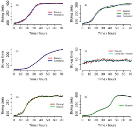
The model was applied to 40 Biolog arrays comprising a total of 3840 time courses. Of these, 2989 exhibited significant growth compared to a known control well. Ac-cording to DIC 598 of these wells were fitted best by the Baranyi model, 2382 by the diauxic model, 9 by the Gompertz model and none by the constant dummy model. The remaining 851 wells exhibited no significant growth, and model fit between the Baranyi, diauxic and Gompertz models was almost arbitrary.
According to BIC the picture is similar, with a slight bias against the diauxic model (2160 diauxic cases with growth) and toward simpler models (793 Baranyi, 36 Gompertz). Again no wells were fitted by the constant dummy model.
Furthermore, in all cases in which the Gompertz model was preferred over Baranyi or diauxic models, DIC scores of these models were very close to each other (within one percent of absolute values). The converse was not the case. Best-fit models usually achieved a DIC score in the range of 200 - 400. For cases where the Gompertz model scored best, the mean difference between the Gompertz model and the second-best model was 1.7; Conversely, where the Gompertz model did not score best, the mean difference in BIC score between the best model and the Gompertz model was 658.
● ●●●●●●●●●●●●●●●●●●● ●●●●●● ●●● ●●●● ● ● ●●●●●●●●●●●●●● ●● ●●●● ●●●●● ●●●●●●●●●●●●● ●●●● ●●● ●● ●●● ● ●●● ●●●● ●● ●● ●● ●● ●●● ● ● ● ● ● ● ●● ●●●● ●●●●●●●● ●●●●●●●●●●●● ●●●●●●●●●●●●●●●●●●●●●●●●●●●●●●●●●●●●●●●●●●●●●●●●●●●●●●●●●●●●●●●●●●●●●●●●●●●●●●●●●●●●●●●●●●●●●●●●●●●●●●●●●●●●●●●●●●●●●●●●●●●●●●●●●●●●●●●●●●●●●●●●●●●●●●●●
0 10 20 30 40 50 60 70
100
250
400
Time / hours
Biolog Units Baranyi Gompertz (a) ●●●●●●●●●●●● ● ●●●●●●●● ● ●● ● ● ● ● ● ●●●●●●● ●●●●●●●●●●●●●●●●● ●●● ●●●●● ●●● ●●●● ●●●●● ●●● ●●●●●●●● ●●● ●●●●●●●● ●●●●●●●● ● ●●●●● ●●●●●●●●●●●●●●●● ●●●●● ●● ●●●●●●●●●●●●● ● ●●●●●●●●●●● ●●●●● ●●●●●●●●●●●●●●●●●●●●●●●●●●●●●●●●●●●● ●●●●●●●●●●●●●●●●●●●●●●●●●●●●●●●●●●●●●●●●●●●●●●●●●●●●●●●●●●●●●●●●●●●●●●●●●●●●●● ●●●●●●●●●●●
0 10 20 30 40 50 60 70
100
200
300
Time / hours
Biolog Units Baranyi Diauxic Gompertz (b) ●●● ●●●●●●●●●●●●●●●●●●●●●● ●●●●●●●●●●●●●●●●●●●●●●●●●●●●●●●●●●●●●●●●●●●●●●●●●●●●●●●●●●●●●●●●● ●●●●●●●●●●● ●●●●●●●●●●●●●●● ●●●●●●●●●●●●●●●●●●●●●●●●●●●●● ●●●●●●●●●●● ●●●●●●●●●● ●●●●●● ●●●●●●●●● ●●●●●●●●●●●●●●●● ●●●●●●●●●●●●●●●●●●●●●●●●●● ●●●●●●●●●●●●●●●●●●●●●●●●●●●●●●●●●●●●●●●●●●●●●●●●●●●●● ●●●●●●●●●●●●
0 10 20 30 40 50 60 70
100
200
Time / hours
Biolog Units Baranyi Gompertz (c) ● ● ●● ● ●●●● ● ● ●●●●● ●●●●● ● ● ●● ● ●● ● ● ● ●● ●● ● ● ● ● ● ● ● ● ● ● ● ● ● ● ●● ● ●● ●● ● ● ● ● ●● ● ● ●●●●● ● ● ●● ● ●● ●●● ●●● ●● ● ● ●● ● ●●● ●●● ● ● ● ● ● ●● ●● ●●●● ● ● ● ● ● ● ●● ● ● ● ● ●● ● ●● ●●● ●● ● ● ●●●●● ●●● ● ● ●●● ● ● ● ●●●●● ● ● ●● ● ●● ●● ● ●●●●● ● ● ●●● ● ● ● ● ● ● ● ● ● ●● ●● ●● ● ●●●● ● ● ●●●● ● ● ● ●●● ● ●● ● ● ●●●● ●●●● ●●● ● ● ●●●●●●●●● ● ● ● ●●●●●● ● ● ● ●● ● ● ● ●● ●● ● ●●● ● ● ● ● ● ● ● ● ● ● ●● ● ● ● ● ● ● ●●●●●●●● ● ● ●●
0 10 20 30 40 50 60 70
20
40
60
Time / hours
Biolog Units Diauxic Linear No−Growth (d) ●●●●●●●●●● ●●● ● ●●●●●●●●● ● ● ● ● ● ● ●●●●●●● ●● ● ● ● ● ●● ●●●●●● ●●● ● ●● ● ● ●● ● ● ● ● ●●● ● ●●●● ● ●●● ●●● ● ● ● ●● ●●● ●● ● ●●●●● ●● ● ●●●● ●● ●● ●●● ● ● ●●●●● ● ●● ● ●● ●●●●●● ●●●● ●●●●●●●●●●●●●●●●●●● ● ●●●●●●●● ● ●● ● ●●●●●●●●●● ●●●●●●●●●●●● ●● ● ●●●● ● ● ●● ● ●●● ●●●●●●●●●●●●●●●●●●●●●●●●●●●●●●●●●●●●●●●●●●●●●●●●●●●●●●● ●●●● ●●●●●●●●●●●●●●●●●● ●●●●●● ● ●●
0 10 20 30 40 50 60 70
100
250
Time / hours
Biolog Units Baranyi Diauxic (e) ●●●●●●●●●●●●●●●●●●●●●●●●●●●●●●●●●●● ●●●●●●●●●●●●●●●●●●●●●●●●●●●●● ●●●●●●●●●●●●●●●●●●●●●●●●●●●●●●●●●●●●●●●●● ●●●●●●●●●●●●●●●●●●●●●●●●●●●●●●●●●●●●●●●●●●●●●●●●●●●●●● ●●●●●●●● ●●●●● ●●●● ●●●●●● ●●●●●●●●●●●●●●●●● ●●●●●●●●●●●●●●●●●●●●●●●●●●●●● ●●●●●●●●●●●●●●●●●●●●●●●●●●●●●●●●●●●●●●●●●●●●●●●● ●●●●●●●●●●●●
0 10 20 30 40 50 60 70
100
250
400
Time / hours
Biolog Units
[image:13.595.167.443.189.450.2]Diauxic (f)
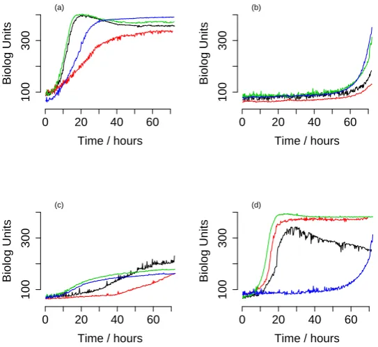
Fig. 3. Example data curves with model fits. (a) A typical data curve where the Baranyi model is best. The Baranyi model fits the data much better than the Gompertz model, that cannot fit either the shape off the lag phase or the shape of the transition to stationary phase. As a consequence, the Gompertz model would overestimate both the length of the lag phase and the maximal growth rate. (b) A typical data curve where diauxic model fits best. Neither the Baranyi nor the Gompertz model can capture the dynamics. (c) A curve with a preferred Gompertz model according to DIC. A fitted Baranyi-curve is also shown. (d) A curve showing no significant growth compared to a control well. Due to a slight increase in coloration this is fitted best equally by a diauxic and Baranyi model. Absence of growth is detected by comparing to the control well. (e) A borderline case that shows slight diauxic behavior. (f) Diauxic curve with high growth ons2.
Table 1. BIC scores for the relevant models in figure??.
Strain DIC Baranyi DIC Diauxic DIC Gompertz DIC No-Growth
(a) P105-A12 388.5 398.0 2497.8 361073
(b) P106-E01 5457.6 431.1 5819.9 376824
(c) P107-G03 123.3 123.1 123.0 272838
(d) P106-H12 114.4 114.2 120.8 258
(e) P106-B11 548.1 401.7 555.5 135383
[image:13.595.157.465.644.723.2]Further evidence for the value of the Baranyi model and Baranyi lag term in the diauxic model in fitting this type of data can be seen from the relative wide spread of the estimated mean for the curvature parameter of the lag phase, ν in both models, as well as the curvature parameterm in the Baranyi model (Figure
??). Thus we consider it likely that any model lacking such an extra parameter would fail to accommodate the range of curve shapes we have encountered.
Histogram for parameter m in Baranyi model
Log(m)
Frequency
0 1 2 3
0
20
40
60
Histogram for parameter nu in Baranyi model
Log(nu)
Frequency
−5 −4 −3 −2 −1 0 1
0
20
40
60
Histogram for parameter nu in diauxic model
Log(nu)
Frequency
−3 −2 −1 0 1 2
0
100
200
[image:14.595.157.424.281.559.2]300
Fig. 4. Histograms form,ν in the Baranyi andν in the diauxic model, for curves where these were the respective best-fit model and where significant growth was detected. The wide spread of these distributions is indicative of the importance of these parameters in fitting a range of data.
3.2. Identification of curve features beyond AUC
important, as such strains or conditions could speed production and/or cut costs. Figures ??(a) and??(b) show the curves with the shortest and longest lag phases respectively. These curves have quite different AUCs and maximal outputs so would be difficult to identify without a suitable modeling approach. Similarly, figures??(c) and??(d) show the curves with the fastest and slowest maximal growth. These too would be difficult to identify without a robust modeling approach.
0 20 40 60
100
300
Time / hours
Biolog Units
(a)
0 20 40 60
100
300
Time / hours
Biolog Units
(b)
0 20 40 60
100
300
Time / hours
Biolog Units
(c)
0 20 40 60
100
300
Time / hours
Biolog Units
[image:15.595.168.440.294.543.2](d)
Fig. 5. Example data curves with potentially useful derived parameters. Some of the curves in the data set with (a) shortest lag phase, (b) longest lag phase, (c) lowest maximum growth rate (while still exhibiting significant growth) and (d) highest rate.
Table 2. The AUC and mean estimated pa-rameters for the four strains shown in figure 1.
Strain AUC L µmax A
P101-D06 190.6 32.6 15.3 301.2 P102-E11 190.7 10.1 9.5 163.3 P103-C05 191.5 21.7 18.1 219.5 P104-C12 192.3 16.6 6.6 162.0
We have found that a comparison to the 95% quantile of maximum coloration of a control well works reliably in identifying whether growth occurs.
3.3. The estimated parameters and model-independent measurements are reliable
The Bayesian approach has allowed us to use the posterior distributions to estimate standard deviations of the individual model parameters as well as the numerically derived model-independent growth measurements. These are generally low (typi-cally < 1% of the parameter values) and are elevated only in cases where some parameters are not estimable from the data, e.g. estimation ofymaxwhen fitting a Baranyi model to data that is cut off before stationary phase is reached (standard deviation as high as 10% of the parameter), but also sometimes s1 and s2 when fitting the diauxic model to data clearly depicting simple growth.
We have found thatA(the maximum colouration change) very closely matches the respective model parameter(s), and thatµmax has given good comparability of results between wells even with different best-fit models. In cases of diauxic growth, particularly with smalls2 and the bulk of growth on s1 (as is the case in the vast majority of diauxic cases observed) the Baranyi model would sometimes give an artificially low estimate ofµmaxas it tries to compensate for the (in a sense slower) two-step approach to peak coloration by fitting an altogether slower curve. Figure
where s1is effectively depleted.
While our descriptive measurementsL,µmaxandAgive us consistent definitions and readily comparable results for the vast majority of cases, the various model pa-rameters we are also inferring allow us a more explanatory analysis of subsets of (or even individual) cases. For instance, within a set of diauxic curves, our estimates of s1 and s2 allow us to identify cases in which the bulk of growth is on the sec-ond substrate. Again, in industrial research applications this may be of particular interest. Similar analysis could be carried out e.g. on the curvature parameters of the Baranyi model, to identify outliers in lag phase behaviour.
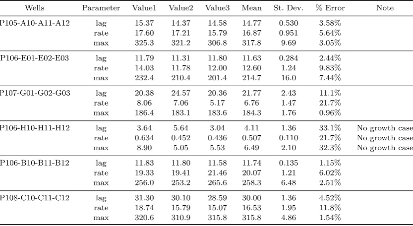
As a further test of reliability, we have compared parameter estimates from wells measuring the same conditions: each condition on these particular phenotype arrays appears in triplicate. For the best fit data shown in Figure??, this provides three independent estimates for each of the three derived parameters for six models, a to-tal of 18 comparisons. The parameter estimates were generally very consistent, with median percentage error of 5.8%. The worst case is for Figure ??(d), where there is no growth, and the parameter estimates vary by approximately 30%; however, because there is no growth, this is not a problem. Full details of these comparisons are provided in Appendix D.
3.4. Performance
The MCMC methodology based on an Adaptive Metropolis algorithm performed well in combination with the models we used. We tested all the Markov chain outputs for the model fits that appear in all figures for convergence using the Hei-delberger and Welch’s convergence test as implemented in the CODA package in R (https://cran.r-project.org/web/packages/coda/index.html). The results from this test showed that all the chains have passed the test, i.e. have converged to the stationary distribution. The outputs are not especially interesting (many tables of non-significant p-values) so we have placed one example in Appendix E and have not included the other outputs.
0 2000 4000 6000 8000 10000
32.5
33.0
33.5
34.0
34.5
35.0
35.5
Iterations
P
ar
ameter V
[image:18.595.159.430.209.452.2]alue
Fig. 6. Initial segment from the trace plot forλfor one AM chain. It is easy to see that the initial acceptance rate is far from optimal, but rapidly improves after the first 2500 iterations.
3.5. Comparison to previous approaches
Vaaset al.2012 discuss one particular case (their figure 4, left hand side) where their model-fitting approach fares worse than their alternative spline-based method. It appears to us that the curve in question is simply diauxic in nature, and we expect that our approach would be able to fit this time course and identify the behaviour as diauxic. The second example they discuss (right hand side of the same curve) could equally likely be fitted by our methodology with an appropriate model. In either case?’s approach likely could not be extended easily to encompass such additional models, using a third-party software package to do the actual parameter estimation.
4. Conclusion
Our solution has several key advantages. Firstly, the Bayesian framework in which our approach operates affords us a great deal of flexibility in extracting in-formation from respiration curves. As we are approximating the joint posterior distribution of all model parameters, we are free to perform further analysis on this and can for instance derive the distribution of arbitrary functions of our model pa-rameters from them. Model choice criteria allow us to readily identify qualitatively different behaviour in the data on top of quantitative measurements. This gives us a “best of two worlds” solution encompassing both unified model-independent descriptive measurements as well as more explanatory model-specific ones.
Secondly, the Baranyi model provides an excellent model to fit a wide range of observed growth curves. The only exception we encountered were curves exhibiting diauxie. In these cases, our diauxic model provided us with good fits in these cases as well. In particular, these two models outperform traditional growth models in many cases. Our modular implementation allows us to adapt our code to new types of experimental data with minimal effort. As PM machinery is being used in a wide range of different areas, this allows our solution to remain applicable as new types of data become available.
Thirdly, the model-independent measurementsL, µmax and A we derive from the fitted curves allow an immediate comparison of key values between different time series, even if qualitatively different models were used to fit the data. This allows us to match simpler (e.g. spline-based) approaches in their ability to per-form quantitative comparisons between a wide range of growth behaviors. However in addition, our approach retains information from the richer model-dependent pa-rameters. This gives us powerful tools to perform further analysis on specific subsets of data. In particular, we can use these to compare wells with qualitatively similar behaviour in more detail, for instance utilisation of different substrates in diauxic curves.
Lastly, our implementation is suited to high-throughput analysis of PM data. Compared to previous approaches to data analysis on PM experiments, we believe that our solution offers improvements in several areas. Even the relatively small number of models we have implemented so far allows our solution to successfully fit a wide range of data.
We believe that our extensible approach is uniquely suited to “keep up” with PM data, as PM machinery is being used for an increasingly wide field of different types of experiments. As PM machinery continues to find novel usage scenarios, the modular implementation we have chosen will allow our solution to remain flexible in accommodating data from these scenarios.
5. Billing address
Program Code Availability
We have made the program code
available on GitHub at URL https://github.com/dovstekellab/mcmc-pma.git un-der license GNU GPLv3. We also include instructions on how to compile and run the code, as well as how to interpret the results files.
Acknowledgments
We thank SABMiller for their support of this research project. Some preliminary work on fitting growth models to PM data using an MCMC approach was also carried out by Ewan Johnstone on a BBSRC-funded summer studentship at the University of Nottingham. MG is currently recipient of a DOC Fellowship of the Austrian Academy of Sciences.
Appendix A. Prior distributions
We used uninformative or uniform priors as follows:
(1) For models that feature a lag parameter λ, we assumed 0≤λ≤dim(x). (2) For all parameters where we were not dealing with their logarithm anyways, we
assumed that they are positive.
(3) Where applicable we assumedymax> y0.
(4) In the full Baranyi model, we requiredr > ν,m >1, as otherwise these param-eters were usually inestimable due to high correlation. Similarly in the Baranyi models where only one ofν,mare fixed.
(5) For all other parameters, we used improper uniform priors without any bounds.
Appendix B. Estimation of initial parameters
The heuristics we used to estimate initial parameter vectors are as follows: (1) For initial cell concentration, we took the average of the first ten data points.
Similarly for the maximum concentration, we took the average of the maximum of any ten-point interval in the time series.
(2) For the lag parameter, we fit lines to every 20-point interval of data points, and intersected the maximum-slope line withy=y0, withy0 derived as in the previous line.
(3) For the growth rater, we used a simple search heuristic to guess an initial value that we have found empirically to be effective. We start from a sufficiently large interval of possible values [rmin, rmax], and divided this into ten equal parts
(4) For the remaining parameters we used the same search algorithm, except we compared the sum of squares of differences between modeled and observed data instead of maximum slope.
Specific to each of the models we did the following: We used [0.01,1], [2,10], [0.3,1] as initial intervals for r, m, ν in this search algorithm. We first called this forr, setting both remaining parameters to 1, then similarly for the remaining ones. For the diauxic models, we proceed similarly, except we additionally needed to find
s1 ands2, respectively the division of the total growth between the two. To do so, we found the maximum slope on a smoothed curve as in our estimation for the lag parameter, and then the minimum slope between that point and when the smoothed curve first comes within 12 standard deviations of the maximum. (In other words, we looked for the characteristic intermittent slowing-down of growth.) We then subtracted y0 from the value at this point, and took this as the initial guess for
s1. For the remaining parameters we proceeded similarly as in the Baranyi model, using [10−8,10−4],[0.05,1],[0.0001,11] as initial intervals forr1,ν,k
1 in the search algorithm. We always use 0.0003 forr2, as performing our search heuristic for this parameter did not improve results.
Appendix C. Estimation of measurement error from data
We took a smoothed curve (taking the average of every nine adjacent measurements; without taking logarithms) as reference to numerically estimate the variance. We however always assumed a minimum variance of 5 Biolog units. That is, we defined
σ2= min{5,dim(x)1 Pdim(x)−5
j=4 xj−19(xj−4+xj−3+· · ·+xj+4)} .
Appendix D. Consistency analysis
Table 3. Parameter estimate consistency
Wells Parameter Value1 Value2 Value3 Mean St. Dev. % Error Note
P105-A10-A11-A12 lag 15.37 14.37 14.58 14.77 0.530 3.58%
rate 17.60 17.21 15.79 16.87 0.951 5.64%
max 325.3 321.2 306.8 317.8 9.69 3.05%
P106-E01-E02-E03 lag 11.79 11.31 11.80 11.63 0.284 2.44%
rate 14.03 11.78 12.00 12.60 1.24 9.83%
max 232.4 210.4 201.4 214.7 16.0 7.44%
P107-G01-G02-G03 lag 20.38 24.57 20.36 21.77 2.43 11.1%
rate 8.06 7.06 5.17 6.76 1.47 21.7%
max 186.4 183.1 183.6 184.3 1.76 0.96%
P106-H10-H11-H12 lag 3.64 5.64 3.04 4.11 1.36 33.1% No growth case
rate 0.634 0.452 0.436 0.507 0.110 21.7% No growth case
max 8.90 5.05 5.53 6.49 2.10 32.3% No growth case
P106-B10-B11-B12 lag 11.83 11.80 11.58 11.74 0.135 1.15%
rate 19.33 19.41 21.46 20.07 1.21 6.02%
max 256.0 253.2 265.6 258.3 6.48 2.51%
P108-C10-C11-C12 lag 31.30 30.10 28.59 30.00 1.36 4.52%
rate 18.74 15.79 15.07 16.53 1.95 11.8%
max 320.6 310.9 315.8 315.8 4.86 1.54%
Appendix E. Convergence tests
Convergence for all of the Markov chains for model fits used in the figures was carried out using the Heidelberger and Welch’s convergence test as implemented in the CODA package in R (https://cran.r-project.org/web/packages/coda/index.html). All of the chains passed the test, i.e. demonstrating convergence to a stationary distribution. The output for each chain is in the form of a table with a p-value for each parameter. An example from one chain that is typical of all output is:
Table 4. Example convergence test output from CODA Variable Stationarity Test Start Iteration p-value
V1 passed 1 0.357
V2 passed 1 0.547
V3 passed 1 0.560
V4 passed 1 0.297
V5 passed 1 0.602
V6 passed 1 0.853
V7 passed 1 0.218
V8 passed 1 0.173
[image:22.595.195.405.579.679.2]hypothesis has been accepted for all variables in the chain. We obtained similar results for all of the Markov chains tests (data not shown).
References
1. Andrieu C, Atchad´e Y, On the efficiency of adaptive mcmc algorithms,Proceedings of the 1st international conference on Performance evaluation methodolgies and tools, ACM, p. 43, 2006.
2. Andrieu C, Thoms J, A tutorial on adaptive mcmc, Statistics and Computing
18(4):343–373, 2008.
3. Atchad´e Y, Fort G, Limit theorems for some adaptive mcmc algorithms with subge-ometric kernels,Bernoulli 16(1):116–154, 2010.
4. Bai Y, Roberts G, Rosenthal J, On the containment condition for adaptive Markov chain Monte Carlo algorithms,Tech Rep, University of Warwick. Centre for Research in Statistical Methodology, 2009.
5. Baranyi J, Simple is good as long as it is enough,Food Microbiology 14(4):391–394, 1997.
6. Baranyi J, Roberts T, A dynamic approach to predicting bacterial growth in food,
International journal of food microbiology 23(3):277–294, 1994.
7. Baranyi J, Roberts T, Mathematics of predictive food microbiology, International journal of food microbiology26(2):199–218, 1995.
8. Baranyi J, Roberts T, McClure P, A non-autonomous differential equation to model-bacterial growth,Food Microbiology 10(1):43–59, 1993.
9. Bochner B, New technologies to assess genotype–phenotype relationships,Nature Re-views Genetics4(4):309–314, 2003.
10. Bochner B, Global phenotypic characterization of bacteria, FEMS microbiology re-views33(1):191–205, 2009.
11. Bochner B, Gadzinski P, Panomitros E, Phenotype microarrays for high-throughput phenotypic testing and assay of gene function, Genome Research 11(7):1246–1255, 2001.
12. DeNittis M, Querol A, Zanoni B, Minati JL, Ambrosoli R, Possible use of biolog methodology for monitoring yeast presence in alcoholic fermentation for wine-making,
J Appl Microbiol 108:1199–1206, 2009.
13. DeNittis M, Zanoni B, Minati JL, Gorra R, Ambrosoli R, Modelling biolog profiles’ evolution for yeast growth monitoring in alcoholic fermentation,Lett Appl Microbiol
52:96–103, 2010.
14. Eddy SR, What is bayesian statistics?,Nature biotechnology22(9):1177–1178, 2004. 15. Gamerman D, Lopes H, Markov chain Monte Carlo: stochastic simulation for
Bayesian inference, Chapman & Hall/CRC, 2006.
16. Gelman A, Carlin JB, Stern HS, Dunson DB, Vehtari A, Rubin DB, Bayesian data analysis, CRC press, 2013.
17. Gilks W, Richardson S, Spiegelhalter D,Markov chain Monte Carlo in practice, Chap-man & Hall/CRC, 1996.
18. Haario H, Saksman E, Tamminen J, An adaptive metropolis algorithm,Bernoulli pp. 223–242, 2001.
19. Hastings WK, Monte carlo sampling methods using markov chains and their applica-tions,Biometrika57(1):97–109, 1970.
21. Kahm M, Hasenbrink G, Lichtenberg-Frat´e H, Ludwig J, Kschischo M, grofit: fitting biological growth curves with r,Journal of Statistical Software 33(7):1–21, 2010. 22. Kompala D, Ramkrishna D, Jansen N, Tsao G, Investigation of bacterial growth on
mixed substrates: experimental evaluation of cybernetic models, Biotechnology and Bioengineering 28(7):1044–1055, 1986.
23. Kompala D, Ramkrishna D, Tsao G, Cybernetic modeling of microbial growth on multiple substrates,Biotechnology and bioengineering 26(11):1272–1281, 1984. 24. Lopez S, Prieto M, Dijkstra J, Dhanoa M, France J, Statistical evaluation of
math-ematical models for microbial growth, International journal of food microbiology
96(3):289–300, 2004.
25. Peleg M, Corradini MG, Microbial growth curves: what the models tell us and what they cannot,Crit Rev Food Sci Nutr 51(10):917–945, 2011.
26. Richards F, A flexible growth function for empirical use, Journal of experimental Botany10(2):290–301, 1959.
27. Schwarz G, Estimating the dimension of a model,The annals of statistics 6(2):461– 464, 1978.
28. Spiegelhalter DJ, Best NG, Carlin BP, Van Der Linde A, Bayesian measures of model complexity and fit,Journal of the Royal Statistical Society: Series B (Statistical Methodology)64(4):583–639, 2002.
29. Torres NP, Lee AY, Giaever G, Nislow C, Brown GW, A high-throughput yeast as-say identifies synergistic drug combinations,Assay Drug Dev Technol11(5):299–307, 2013.
30. Vaas L, Sikorski J, Michael V, G¨oker M, Klenk H, Visualization and curve-parameter estimation strategies for efficient exploration of phenotype microarray kinetics,PloS one 7(4):e34846, 2012.
31. Vehkala M, Shubin M, Connor TR, Thomson NR, Corander J, Novel R Pipeline for Analyzing Biolog Phenotypic Microarray Data,PloS one10(3): e0118392, 2015. 32. Zhou L, Lei X, Bochner B, Wanner B, Phenotype microarray analysis of escherichia
coli k-12 mutants with deletions of all two-component systems,Journal of bacteriology
185(16):4956–4972, 2003.