Changes in VED–modelling

(1)

Changes in VED – modelling

The aim of the modelling exercise is to help gain an understanding of whether increases in differential between VED bands would help the UK achieve its:

1) two targets relating to lower carbon cars1

2) commitment to a 20% reduction in carbon emissions by 2010.

Base Case

To help model the impact that changes in the differential between bands would have, two ‘base cases’ were developed. These used current new vehicle purchase data as a starting point and factored this data up to take into account annual expected efficiency improvements and anticipated changes in purchasing patterns. The new vehicle data was for both private and company cars and differentiated by CO2 emissions (SMMT, 2004). An example of the data used is provided below in Table 1.

Table 1 Company car New Vehicles - Total Registrations 2004 by CO2 (g/km) Sales Type CO2 (g/km) Total Registrations 2004

Company 80 2.00

Company 87 4

Company 104 572

Company 107 432

Company 109 1425

Company 110 1373

Source: Society of Motor Manufacturers and Traders (2004)

The assumptions used with regard to efficiency and purchasing patterns are based on historic trends and differentiate between company and private vehicles. Assumptions are detailed below in tables 2 and 3. Table 2 assumptions reflect that efficiency gains are easier in larger less fuel-efficient vehicles than smaller vehicles.

Table 2 Assumptions regarding efficiency improvements Vehicles (emissions per

kilometre) Efficiency improvements per annum

Base 1 (more improvements) Base 2 (less improvements)

Less than 150 grams 1.50% 0.50

Between 151 to 200 grams 2.00% 0.75

Between 201 to 250 grams 2.00% 0.75

Greater than 251 grams 2.50% 1.00

(2)

[image:2.595.65.436.122.300.2]

Table 3 Assumptions regarding changes in purchasing patterns (increases in the number of vehicles per annum)

Base Case 1 (more efficiency improvements)

Base Case 2 (less efficiency improvements)

Current vehicle emissions (per kilometre)

Company Private Company Private

Less than 150 grams 3.00% 5.00% 2.00% 3.50% Between 151 to 200

grams 2.00% 1.00% 1.00% 1.00%

Between 201 to 250

grams 1.00% 1.00% 1.00% 1.00%

Greater than 251

grams 2.00% 4.00% 2.00% 3.50%

Summary results from the development of the base data spreadsheet model are shown in Table 3 and Table 4.

[image:2.595.67.466.416.590.2]

Table 3 reflects the trend for the purchase of smaller and larger vehicles particularly in the private car. It also reflects the overall increase in the purchase of new cars.

Table 4 - Company Car registrations by VED band for 2008 and 2012 under base case 1 and 2 (i.e. assuming efficiency improvements and changes in purchasing patterns)

VED

band COfigure 2 emission grams per kilometre

2004* 2008 Base Case 1

2008 Base Case 2

2012 Base Case 1

2012 Base Case 2

AAA Up to 100 6 651 6.5 12814 1959

AA 101-120 39425 90898 52779 154737 72817

A 121-150 394506 737109 597760 1018172 679714

B 151-165 351470 240890 255159 238944 198214

C 166-185 261414 227940 271167 123915 178963

D 185 + 320382 204192 268927 132459 301492

Total 1367203 1501680 1445799 1681041 1547546 Average carbon emissions 168.93 156.24 164.10 144.91 159.36 Percentage of vehicles

(3)

[image:3.595.69.464.137.339.2]

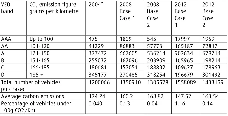
Table 5 - Private Car registrations by VED band under base case 1 and 2 (i.e. assuming efficiency improvements and changes in purchasing patterns)

VED

band COgrams per kilometre 2 emission figure 2004* 2008 Base Case 1

2008 Base Case 2

2012 Base Case 1

2012 Base Case 2

AAA Up to 100 475 1809 545 17997 1959

AA 101-120 41229 86883 57773 165187 72817

A 121-150 377472 667605 536214 902634 679714

B 151-165 255032 167096 203909 165965 198214

C 166-185 180681 157051 188832 109627 178963

D 185 + 345177 270465 318254 196679 301492

Total number of vehicles

purchased 1200066 1350910 1305528 1558089 1433159

Average carbon emissions 174.24 160.2 168.82 147.52 163.54 Percentage of vehicles under

100g CO2/Km 0.040 0.13 0.04 1.16 0.14

Changes in VED

Two scenarios were developed and utilised to help assess the impact that changes in VED might have. Key features of the scenarios are

Table 6 Key features of VED change scenarios

Scenario 1 Scenario 2

Introduction of a new top band E (220 +) Introduction of a new top band E (220 +) All car registrations are potentially

impacted Only cars in the bottom and top 10 grams of a band are impacted Percentage change between impacted cars

is detailed in Table 7

Percentage change between impacted cars is detailed in Table 12. Higher than scenario 1 Impact differs depending on size of vehicle Impact differs depending on size of vehicle

Scenario 2 with its impact on the bottom and top 10 grams of each band can be considered a more ‘pessimistic’ scenario and Scenario 1 a more ‘optimistic scenario’. The scenarios, and their impact on the two base cases are detailed below.

Scenario 1

Scenario 1 assumes that all vehicles within a band are potentially impacted by changes in VED. I.e. vehicles at the top end of band are as likely to move to the band below as vehicles at the bottom end of the band.

It assumes that significant change in the VED differential between bands would result in a substantial movement between bands. The assumption is based on Mori research (DfT, 2003), which suggests that if there were a £300 differential between each VED band 72% of people would swap bands. The research also suggests that people who currently own a larger vehicle would be less likely to swap. The research was used to inform the development of our

(4)

Furthermore, band D would change from covering all vehicles greater than 186 grams of carbon dioxide per vehicle kilometre to covering vehicles in the range 186 – 220. A new top band E was introduced which would cover all vehicles greater than 221 grams of carbon dioxide per

kilometre. Here we assume that vehicles in the range 220-240 would potentially move to band D.

Table 7 Percentage Change assumed in Scenario 1

From To Percentage change

AA AAA 60%

A AA 60%

B A 50%

C B 50%

D now (186-220) C 40%

New band E (220 +) D 40%

[image:4.595.66.495.340.731.2]

The new vehicles purchases, which are transferred to the lower bands, are distributed according to the number of vehicles in the different carbon categories. I.e. the higher the number of existing vehicles the more likely it is people would purchase it if they were moving to the lower band.

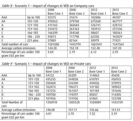
Table 8 - Scenario 1 – impact of changes in VED on Company cars

2008

Base Case 1 2008 Base Case 2 2012 Base Case 1 2012 Base Case 2

AAA Up to 100 55375 31674 102886 40107

AA 101-120 478563 379768 675568 467777

A 121-150 415165 366684 526741 428132

B 151-165 234415 263163 183912 257236

C 166-185 166399 204548 98607 180361

D 186 - 220 93873 117798 62350 102029

E 221 plus 57889 82164 30979 71921

Total number of cars 1501680 1445799 1681041 1547564 Average carbon emissions 144.28 152.18 132.48 147.20 Percentage of cars under 100

gram CO2 per km 3.69 2.19 6.12 2.59

Table 9 - Scenario 1 – impact of changes in VED on Private cars

2008

AAA Up to 100 54122 35209 114063 45650

AA 101-120 435255 344838 610701 436955

A 121-150 350468 316440 444036 370993

B 151-165 162074 196371 141182 189822

C 166-185 137255 161437 101185 151646

D 186 - 220 109780 119297 85057 114305

E 221 plus 101956 131936 61865 123788

Total Number of

cars 1350910 1305528 1558089 1433159

Average carbon emissions 148.08 157.11 135.66 151.51 Percentage of cars under 100

(5)

Table 10 - Scenario 1 – Company car - difference in average carbon emissions (comparison with base case)

2008 2012

Base Case 1 Base Case 2 Base Case 1 Base Case 2

Base Case 156.24 164.10 144.91 159.36

Scenario 1 Average carbon

emissions 144.28 152.18 132.48 147.20

[image:5.595.65.492.251.338.2]

Difference 11.96 11.92 12.43 12.16

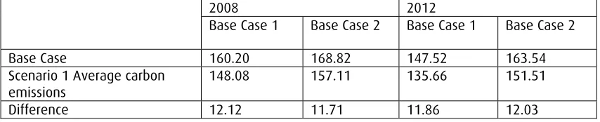
Table 11 – Scenario 1 – Private car – difference in average carbon emissions (comparison with base case)

2008 2012

Base Case 160.20 168.82 147.52 163.54

emissions 148.08 157.11 135.66 151.51

Difference 12.12 11.71 11.86 12.03

Scenario 2

Scenario 2 assumes that movements between bands would only be from the lowest 10 grams of a band to the highest 10 grams of the band below. The proportions of movement between these sections of the bands are detailed in Table 12. The percentage change is slightly higher than that used in Scenario to reflect that the application of the percentage change applies to a much smaller number of vehicles.

Table 12 – Scenario 2 changes in Vehicle purchasing patterns due to changes in VED

From To Percentage change

AA AAA 70%

A AA 70%

B A 60%

C B 50%

D now (186-220) C 50%

New band E (220 +) D 40%

As with Scenario 1 a new band D would change from covering all vehicles greater than 186 grams of carbon dioxide per vehicle kilometre to covering vehicles in the range 186 – 220. A new band E would be introduced which would cover all vehicles greater than 221 grams of carbon dioxide per kilometre

(6)

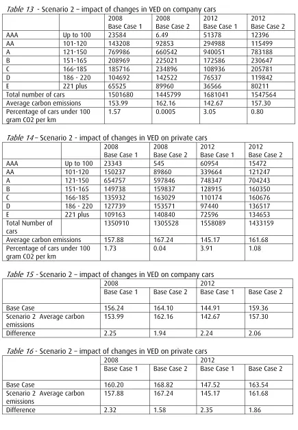
Table 13 - Scenario 2 – impact of changes in VED on company cars

2008

AAA Up to 100 23584 6.49 51378 12396

AA 101-120 143208 92853 294988 115499

A 121-150 769986 660542 940051 783188

B 151-165 208969 225021 172586 230647

C 166-185 185716 234896 108936 205781

D 186 - 220 104692 142522 76537 119842

E 221 plus 65525 89960 36566 80211

Total number of cars 1501680 1445799 1681041 1547564 Average carbon emissions 153.99 162.16 142.67 157.30 Percentage of cars under 100

[image:6.595.62.497.105.732.2]

gram CO2 per km 1.57 0.0005 3.05 0.80

Table 14 – Scenario 2 - impact of changes in VED on private cars

2008

AAA Up to 100 23343 545 60954 15472

AA 101-120 150237 89860 339664 121247

A 121-150 654757 597846 748347 704243

B 151-165 149738 159837 128915 160350

C 166-185 135932 163029 110174 160676

D 186 - 220 127739 153571 97440 136517

E 221 plus 109163 140840 72596 134653

Total Number of

cars 1350910 1305528 1558089 1433159

Average carbon emissions 157.88 167.24 145.17 161.68 Percentage of cars under 100

gram CO2 per km 1.73 0.04 3.91 1.08

Table 15 - Scenario 2 – impact of changes in VED on company cars

2008 2012

Base Case 156.24 164.10 144.91 159.36

emissions 153.99 162.16 142.67 157.30

Difference 2.25 1.94 2.24 2.06

Table 16 - Scenario 2 – impact of changes in VED on private cars

2008 2012

Base Case 160.20 168.82 147.52 163.54

emissions 157.88 167.24 145.17 161.68

(7)

[image:7.595.67.536.138.329.2]

Results

Table 17 Percentage of vehicles which are 100g of CO2/km or lower in 2012

Base Case 1 Average

(weighted to take into account number of vehicles)

Base Case 2 Average (weighted to take into account number of vehicles) No change in VED

Company 0.35 0.044

Private 1.16 0.73

0.14

0.09

Scenario 1

Company 6.12 2.59

Private 7.32 6.69

3.19

2.87

Scenario 2

Company 3.06 0.80

Private 3.91

3.47

1.08

0.93

Commitment to a 20% reduction in carbon emissions by 2010

We have modelled the impact of changes in VED under two different scenarios and base cases. A more ‘optimistic’ scenario (1) and more ‘pessimistic’ scenario (2) have been tested. The results suggest that average carbon reductions in the range of 2 grams/km/vehicle to 12

grams/km/vehicle may be possible. Below we have modelled the impact that this would have on overall carbon emission reductions, by examining the number of vehicle kilometres that would be impacted under two scenarios. Table 18 assumes that the percentage of vehicles impacted is related to the replacement of the vehicle stock by new vehicles. New vehicles take up 10% of vehicle stock. It is assumed that people drive the average number of kilometres. I.e. 10% of the vehicle stock is replaced each year and this correspondingly impacts on vehicle kilometres - 10% in 2008, 20% in 2009, and 30% in 2010. Table 19 takes into account that it is highly probable that new car owners (private and company) will drive more than the average number of kilometres.

Table 18 New car vehicle purchases – average emissions in 2008 Base Case 1 Average

(weighted to take into account number of vehicles)

Base Case 2 Average

(weighted to take into account number of vehicles) No change in VED

Company 156.24 164.10

Private 160.20 158.10

168.82

166.34

Scenario 1

Company 144.28 152.18

Private 148.08 146.04

157.11

154.51

Scenario 2

Company 153.99 162.16

Private 157.88

155.83

167.24

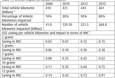
[image:7.595.66.536.547.743.2]

(8)

[image:8.595.65.435.107.358.2]

Table 19 Overall impact on carbon emissions

2008 2010 2012 2015

Total vehicle kilometre

(billion) 2 418 431 443 461

Percentage of Vehicle kilometres impacted

10% 30% 50% 80%

Number of vehicle

kilometre impacted (billion)

41.8 129.30 221.5 368.8

CO2 saving per vehicle kilometre and impact in terms of MtC* 2 grams

Saving in MtC 0.02 0.07 0.12 0.15 5 grams

(9)

[image:9.595.65.440.98.346.2]

Table 20 Potential MtC savings under a number of gram reduction per vehicle kilometre

2008 2010 2012 2015

Total Billion vehicle

kilometre 418 431 443 461

Percentage of vehicle

kilometre impacted 20% 60% 80% 100% Number of vehicle

kilometre impacted (billion) 83.6 258.6 354.4 461 CO2 saving per vehicle kilometre and impact

2 grams

Saving in MtC 0.27 0.85 1.16 1.51

* Calculation of MtC – Example

Billion car vehicle kilometres x carbon dioxide (grams) saving per kilometre 41.8 x 2 = 83600000000 grams of carbon dioxide

Conversion into tonnes = 83600000000 / 1000000

= 83600 tonnes of carbon dioxide Conversion into million tonnes = 83600/ 1000000

= 0.0836 million tonnes of carbon dioxide

Conversion into tonnes of carbon = 0.0836 x 12 / 44 (atomic mass of C (12) / (atomic mass of CO2 (12 + 16 + 16)

= 0.0228 Limitations

The aim of the above analysis was to gain an understanding of the impact of changes in VED. The approach used is relatively simple but thought appropriate given the timescale available. We are aware that there are limitations to the approach some of which are detailed below:

• The sensitivity range for the base case could be widened.

• There has been no feasibility ‘check’ on movement between bands – e.g. in Scenario 2 base case 2 (2008) the model ‘assumes’ there are no vehicles in the range 90-100 grams there is therefore no movement between band AA and A.

• Scenario 2 assumes movement between lowest 10 grams and highest 10 grams of each band. Smaller ranging bands e.g. B are not treated differently.

(10)

• Does not account for impact on second hand market

• Assumes that same impact on company and private vehicles

Reference

Department for Transport (2003) Assessing the Impact of Graduated Vehicle Excise Duty – Quantitative research