Application of the Hybrid Differential
Transform Method to the Nonlinear
Equations
Inci Çilingir Süngü*, Hüseyin Demir
Department of Mathematics, Faculty of Arts and Sciences, Ondokuz Mayis University, Samsun, Turkey
Email: *[email protected]
Received January 2, 2012; revised February 13, 2012; accepted February 22, 2012
ABSTRACT
In this paper, a hybrid method is introduced briefly to predict the behavior of the non-linear partial differential equa- tions. The method is hybrid in the sense that different numerical methods, differential transform and finite differences, are used in different subdomains. Our aim of this approach is to combine the flexibility of differential transform and the efficiency of finite differences. An explicit hybrid method for the transient response of inhomogeneous nonlinear partial differential equations is presented; applying finite difference scheme on the fixed grid size is used to approximate the space discretisation, whereas the differential transform method is used for time operator. Comparison of the efficiency of the different approaches is a very important aspect of this study. In our test cases, the hybrid approach is faster than the corresponding highly optimized finite difference method in two dimensional computations. We compared our hy- brid approach’s results with the exact and/or numerical solutions of PDE which obtained from Adomian Decomposition Method. Results show that the hybrid approach may be an important tool to reduce the execution time and memory re- quirements for large scale computations and get remarkable results in predicting the solutions of nonlinear initial value problems.
Keywords: Hybrid Differential Transform/Finite Difference Method; Nonlinear Initial Value Problems; Numerical Solution
1. Introduction
Many problems in mathematical physics, theoretical phys- ics, chemical physics and theoretical biology are modeled by the so-called initial value and boundary value pro- blems in the second-order nonlinear partial differential equations. Nonlinear equations also cover the cases of the following types: surface waves incompressible fluids, hydro magnetic waves in cold plasma, acoustic waves in inharmonic crystal, etc. However, these equations are difficult to be solved analytically and sometimes it is impossible then application must be made with relevant numerical methods such as shooting method, finite dif-ference etc. In recent years, differential transform method has been used to solve this type of equation [1-11].
The differential transform method is a numerical me-thod based on Taylor expansion. This meme-thod constructs an analytical solution in the form of a polynomial which is widely equivalent explicit form of solution. The main advantage of this method is to solve both linear and
non-linear equations without non-linearization. Using differential transform method, we can avoid from complexity of ex-pansions of derivatives and compute derivatives as sym-bolically.
When solving initial value problems, the truncation error produced by the finite difference method is greater than that produced by the differential transform method. Hence, in this work we develop a hybrid method which combines the differential transform and the finite differ-ence method. Using this hybrid method, numerical solu-tion can be obtained from a simple iterative procedure. The hybrid method has an advantage to solve nonlinear equations is examined without using linearization. In the literature, there are other hybrid methods. For example, the method used by Beilina’s [12] study includes both the finite difference and finite element methods.
2. Differential Transform Method
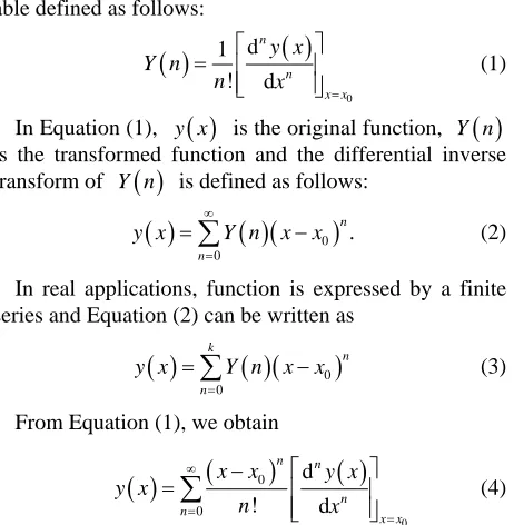
We introduce the main features of the differential trans-formation method [1,5,6,11] according to the differential transform of the nth derivative of a function in one
able defined as follows:
0 d 1 ! d n n x x y x Y nn x
(1)
In Equation (1), y x
is the original function, Y n
is the transformed function and the differential inverse transform of Y n
is defined as follows:
0
0
. n
n
y x Y n x x
(2) In real applications, function is expressed by a finite series and Equation (2) can be written as
00
k
n
n
y x Y n x x
(3) From Equation (1), we obtain
0 0 0 d ! d n n n n x xx x y x
y x n x
(4)Actually Equation (4) implies that the concept of dif-ferential transform is derived from Taylor series expan-sion. Although DTM is not able to evaluate the deriva-tives symbolically, relative derivaderiva-tives can be calculated by an iterative way which is described by the trans-formed equations of the original function. In this study Equation (4) also implies
01
n
n k
y x Y n x x
(5) is negligibly small. In fact k is decided by the conver-gence of natural frequency.After taking differential transformation with respect to time variable, we apply finite difference method to PDE with respect to x variable and their derivatives. The re-gion 0 x a is divided into several equal intervals and each interval has a width h. Take second order accu-rate central difference approximation with respect to the first and second order derivatives, equations are rewritten and computed iteratively. The solutions are compared with the other published numerical solutions of these equations.
3. Illustration of Hybrid Method
To show the effectiveness of the proposed hybrid differ-ential transform method and to give an understandable overview of the methodology three different models of nonlinear differential equations with different initial and boundary conditions will be discussed in the following section. Then our results are compared with published work of Wazwaz [13] in which Adomian decomposition method was used to solve the same equations.
Example 1:
The function u satisfies the nonlinear equation 2 2
2 , 0 1
u u
x
t x
(6)
The initial condition u4x
1x
, 0 x 1, t0and the boundary conditions at and 1, .
0
u x0 0
t
If the equation is expanded and taken the differential
transform of variables u, u t , 2 2 u u x , 2 u x
with
respect to time,
1 1 1 1 0 21 2 1
0
1 , 1 2 , ,
2 , ,
k
k k
k
k F x k F x k F x k k
x x
F x k k F x k x
(7)where F x k
, is differential transformation of u x t
, . Then the central finite difference method is applied to the Equation (7), we get
1
1
1 1 1 1 1 1 1 1
0
1 1 1 1 1
1 2
0
1 2
1 2 2
2
,
i k
i i i i
k
k
i i i
i k
F k
F k F k F k k F k k
k h h
F k F k F k
F k k
h
(8) where F ki
F x k
i,
, xi ih. The initial and bound-ary conditions are
0 0, 0,1, 2,
F k k (9)
0, 0,1, 2,M
F k k (10)
20 4 4
i
F ih ih (11)
The process of programming consists of three major steps. First, Fi
0 are determined from the initial con-ditions as well as the boundary concon-ditions. Secondly, for0
k , Fi
1 can be calculated using the iteration for-mula of Equation (8) together with the initial and bound-ary conditions (9)-(11) and F ki
,u x t
for can be achieved sequentially following the same iteration proc-ess. Finally, the solutions of at time
2 k
t
[image:2.595.60.291.88.324.2]Example 2:
Let us consider the following inhomogeneous initial value problem
21 2
2 2
x x
u
u e t e
t x
(12)
, 0 0u x (13)
Substituting the differential transformation F x k
, of u x t
, into Equation (12) gives,
1
1 1
0 2
1 , 1 , ,
2 k
k
x x
k F x k F x k k F x k
x
e k e k
(14)
After discretizating with central difference formula the PDE becomes,
1
2
1 1 1 1
1 0
1 1
1
2
ih ih
i
k
i i
i k
F k e k e k
k
F k F k
F k k
h
2
(15)
and initial condition is
0 iF 0 (16)
where is Kronecker Delta Function and
,
,i i
F k F x k xi ih.
Using second order finite difference method boundary values were obtained as follows,
0 1 2 3
1 2
3 3
3 3
M M M M
F k F k F k F k
3
F k F k F k F k
Evaluating the recurrence relation in Equation (15) and transformed initial condition (16) and computed bound-ary values, F ki
for are easily obtained anduse the inverse transformation rule in DTM. Then we had the numerical solution and compared with other pub-lished work of Wazwaz [13]. As shown in Table 2, our simulation results exactly coincide with the ADM solu-tions.
2 k
Example 3:
We will consider the following nonlinear inhomoge-neous advection problem
2
1 1
sin sin 2
2 2
u
u x t x
t x
t
(17)with initial condition
, 0 cos
.u x x (18)
[image:3.595.308.538.111.323.2]Using differential transform method to time variable
Table 1. Comparison of numerical results with the Maple 11 solution at t = 0.01.
x Hybrid Maple 11 Error 0.0 0.0000000 0.0000000 0.0000000 0.05 0.2909183 0.2909181 2 × 10⁻⁷
0.1 0.4319186 0.4319185 10–7
0.15 0.5415206 0.5415205 10–7
0.2 0.6323455 0.6323454 10–7
0.25 0.7078180 0.7078179 10–7
0.3 0.7690838 0.7690837 10–7 0.35 0.8165639 0.8165638 10–7
0.4 0.8504209 0.8504208 10–7
[image:3.595.307.538.362.571.2]0.45 0.8707191 0.8707191 0.0000000 0.5 0.8774831 0.8774830 10–7
Table 2. Comparison of numerical results with ADM solu-tions at t = 0.002 for h = 0.1, ∆t = 0.0001.
x Hybrid ADM Error 0.0 0.0020002 0.002 2 × 10⁻⁷
0.05 0.0021025 0.0021025 0 0.1 0.0022103 0.0022103 0 0.15 0.0023236 0.0023236 0
0.2 0.0024428 0.0024428 0 0.25 0.0025680 0.0025680 0
0.3 0.0026997 0.0026997 0 0.35 0.0028381 0.0028381 0
0.4 0.0029836 0.0029836 0 0.45 0.0031366 0.0031366 0
0.5 0.0032974 0.0032974 0
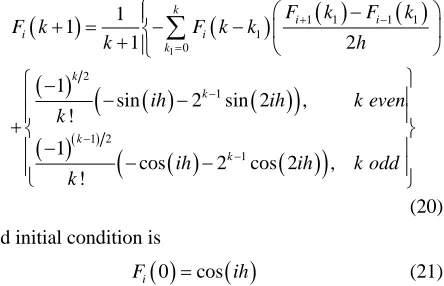
for linear and nonlinear terms of equation, (17) gives
1
1 1
0 2
1
1 2
1
1 , 1 , ,
1
sin 2 sin 2 ,
!
1
cos 2 cos 2 ,
!
k
k k
k
k
k
k F x k F x k k F x k
x
x x k eve
k
x x k odd
k
n (19)
1
1 1 1 1
1 0
2
1
1 2
1
1 1
1
1
sin 2 sin 2 ,
!
1
cos 2 cos 2 ,
!
k
i i
i i
k k
k
k
k
2
F k F k
F k F k k
k
ih ih k even
k
ih ih k odd
k
h
(20) and initial condition is
0 cos
i
F ih (21)
Equation (19) is an iterating process and using this process we get numerical solutions as in Table 3 for and . We compare the solutions of Hybrid Differential Transform with the solutions of Adomian Decomposition Method (Wazwaz [13]). As shown in Table 3, the error between the simulation and ADM results is quite small.
0.1
h t 0.0001
Tables 1-3 show the exact values, the approximation solutions obtained from the hybrid differential transform method and the absolute errors that results from compar-ing the approximate solutions and the Maple 11 or ADM solutions. The Hybrid Method results agree with the pub-lished work of Wazwaz [13], who considered the same equations, for nonlinear initial value problems to six de-cimal places after rounding.
4. Conclusions
[image:4.595.66.288.89.232.2]The hybrid method is employed to predict nonlinear par-tial equations. Some simulation results are illustrated and discussed to compare with other published work. Three
Table 3. Comparison of numerical results with ADM solu-tion at t = 0.001.
x Hybrid ADM Error 0.0 1.0000010 0.9999995 1.5 × 10⁻⁶ 0.05 0.9987007 0.9986997 10× 10–6
0.1 0.9949048 0.9949038 10 × 10–6 0.15 0.9886220 0.9886211 9 × 10⁻⁷
0.2 0.9798683 0.9798674 9 × 10⁻⁷ 0.25 0.9686653 0.9686645 8 × 10⁻⁷
0.3 0.9550412 0.9550404 8 × 10⁻⁷ 0.35 0.9390301 0.9390293 8 × 10⁻⁷
0.4 0.9206717 0.9206711 6 × 10⁻⁷
0.45 0.9000122 0.9000116 6 × 10⁻⁷
0.5 0.8771032 0.8771026 6 × 10⁻⁷
advantages that are briefly explained in this study of this method are as follows:
1) The hybrid method provides an iterative procedure to calculate the numerical solutions; therefore, it is not necessary to carry out complicated symbolic computa-tion.
2) From the nonlinear partial differential equations considered, it has been shown that the proposed method can obtain very accurate numerical approximation.
3) The last and most important advantage is that we do not use linearization in solution procedure. Moreover we can avoid some complex operation therefore; the Hybrid Method provides an iterative procedure to calculate the numerical solutions without using linearization.
It may be concluded that this method is very powerful and efficient in obtaining numerical solutions for these types of partial differential equations with initial condi-tions.
REFERENCES
[1] I. H. A.-H. Hassan, “Differential Transform Technique for Solving Higher Order Initial Value Problems,” Ap-plied Mathematics and Computation, Vol. 154, No. 2, 2004, pp. 299-311. doi:10.1016/S0096-3003(03)00708-2 [2] A. Arikoglu and I. Ozkol, “Solution of Difference
Equa-tions by Using Differential Transform Method,” Applied Mathematics and Computation, Vol. 174, No. 2, 2006, pp. 1216-1228. doi:10.1016/j.amc.2005.06.013
[3] F. Ayaz, “Solution of the System of Differential Equa-tions by Differential Transform Method,” Applied Ma- thematics and Computation, Vol. 147, No. 2, 2004, pp. 547-567. doi:10.1016/S0096-3003(02)00794-4
[4] C. W. Bert and H. Zeng, “Analysis of Axial Vibration of Compound Bars by Differential Transform Method,”
Journal of Sound and Vibration, Vol. 275, No. 3-5, 2004, pp. 641-647. doi:10.1016/j.jsv.2003.06.019
[5] C. K. Chen and S. S. Chen, “Application of the Differen-tial Transform Method to a Non-Linear Conservative System,” Applied Mathematics and Computation, Vol. 154, No. 2, 2004, pp. 431-441.
doi:10.1016/S0096-3003(03)00723-9
[6] C. L. Chen and Y. C. Liu, “Solutions of Two-Boundary- Value Problems Using the Differential Transform Me- thod,” Journal of Optimization Theory and Application, Vol. 99, No. 1, 1998, pp. 23-35.
doi:10.1023/A:1021791909142
[7] H. P. Chu and C. L. Chen, “Hybrid Differential Trans-form and Finite Difference Method to Solve the Nonlin-ear Heat Conduction Problem,” Communication in Non- linear Science and Numerical Simulation, Vol. 13, No. 8, 2008, pp. 1605-1614. doi:10.1016/j.cnsns.2007.03.002 [8] B. L. Kuo, “Applications of the Differential Transform
[9] O. U. Richardson, “The Emission of Electricity from Hot Bodies,” Longman, Green and Co., London, 1921.
[10] Y. L. Yeh, C. C. Wang and M. J. Jang, “Using Finite Difference and Differential Transformation Method to Analyze of Large Deflections of Orthotropic Rectangular Plate Problem,” Applied Mathematics and Computation, Vol. 190, No. 2, 2007, pp. 1146-1156.
doi:10.1016/j.amc.2007.01.099
[11] J. K. Zhou, “Differential Transformation and Its
Applica-tions for Electrical Circuits,” Huazhong University Press, Wuhan, 1986.
[12] L. Beilina, “Adaptive Hybrid Finite Element/Difference Method for Maxwell’s Equations: A Priori Error Estimate and Efficiency,” Applied and Computational Mathemat-ics, Vol. 9, No. 2, 2010, pp. 176-197.