
ISSN Online: 2164-2656 ISSN Print: 2164-2648
DOI: 10.4236/aid.2019.91002 Feb. 21, 2019 8 Advances in Infectious Diseases
Epidemiological Study and Optimal Control for
Lumpy Skin Disease (LSD) in Ethiopia
Okey Oseloka Onyejekwe
*, Abebe Alemu, Biruk Ambachew, Ayalnesh Tigabie
Computational Mechanics and Dynamical Systems Group, Computational Science Program, Addis Ababa University, Arat Kilo Campus, Addis Ababa , Ethiopia
Abstract
Lumpy skin disease (LSD) is an infectious, fatal skin disease of cattle caused by a virus of the family Poxviridae (genus Capripox). In addition, severely af-fected animals suffer from reduced weight, cessation of milk production and infertility. The aim of this paper is to computationally apply epidemiological (SEIR) and optimal control (OC) techniques to study the transmission and the impact of vaccination on LSD. Based on our numerical experiments, we were able to deduce the overall impact of the optimal strategy adopted for this study on the cattle population for vaccination rates within the range of
0≤ ≤
ν
0.85. It is shown that the vaccination as a control strategy signifi-cantly reduced the effects of LSD on the cattle population if properly ma-naged and that an optimal performance of the control strategy adopted here-rin is achieved at an approximate value ofν
=0.6.Keywords
Lumpy Skin Disease, LSD, Optimal Control, Epidemiology, SEIR
1. Introduction
LSD has an economical importance because of permanent damage to hides. It has been reported ([1] [2]) that 10% of animals exposed to LSD experience abor-tion. According to [3], lumpy skin disease (LSD) is an exhaustive viral disease and a pox disease of cattle. It is characterized by fever, nodules on the skin, mucous membranes in internal organs, enlarged lymph nodes and odema of the skin ([3] [4]). Due to chronic debility in affected animals high economic losses occur. The clinical syndrome of LSD was first described in Zambia in 1929. More cases also occurred between 1943 and 1945 in Botswana, Zimbabwe and the republic of South Africa ([1] [3] [5] [6]). Transmission of LSD is by insect How to cite this paper: Onyejekwe, O.O.,
Alemu, A., Ambachew, B. and Tigabie, A. (2019) Epidemiological Study and Optimal Control for Lumpy Skin Disease (LSD) in Ethiopia. Advances in Infectious Diseases, 9, 8-24.
https://doi.org/10.4236/aid.2019.91002
Received: December 28, 2018 Accepted: February 18, 2019 Published: February 21, 2019
Copyright © 2019 by author(s) and Scientific Research Publishing Inc. This work is licensed under the Creative Commons Attribution International License (CC BY 4.0).
http://creativecommons.org/licenses/by/4.0/
DOI: 10.4236/aid.2019.91002 9 Advances in Infectious Diseases vectors (through biting flies) found among cattle sharing similar grazing and watering areas. And those that congregate in the same barn may be contami-nated by the viruses in saliva of the infected animals or ingestion of already con-taminated food or by teratogenic agents and suckling calves ([7] [8]). The inci-dence of LSD occurrence is high during wet seasons [3].
LSD was first observed in Ethiopia in the northwestern part of the country (southwest of Lake Tana) in 1983, [1]. It occurs in all agro-climatic conditions and has the potential to extend its boundaries. Good understanding of epidemi-ology, economic significance and control mechanisms of the disease will en-hance suitable control measures. The disease could be diagnosed using appro-priate serological and molecular techniques. Effective control measures can be achieved through mass vaccination, separation and culling of infected animals, ([9] [10] [11]). It is therefore important to formulate an LSD model with optimal control policy to eradicate LSD epidemic and minimize the cost associated for vaccination strategy [3].
Most studies of epidemic control of LSD focus on increasing immunization coverage (vaccination coverage) in a population to control the disease, but they do not consider how this parameter affects the strategy over a period of time. Though some of these studies have considered vaccination strategy at different levels of immunization, none of them has studied optimal vaccination strategy for LSD disease in Ethiopia. Hence the general objective of this study aims at addressing these shortfalls in order to make the number of infected animals as small as possible.
2. Epidemiological Model Formulation
SEIR Model and Equation Formulation
All Epidemiological ODE models of disease transmission are continuous time compartment level models [12]. The model considered herein is compartmenta-lized into:
S: susceptible portion of population, E: exposed population.
I: the infected population. R: the recovered population.
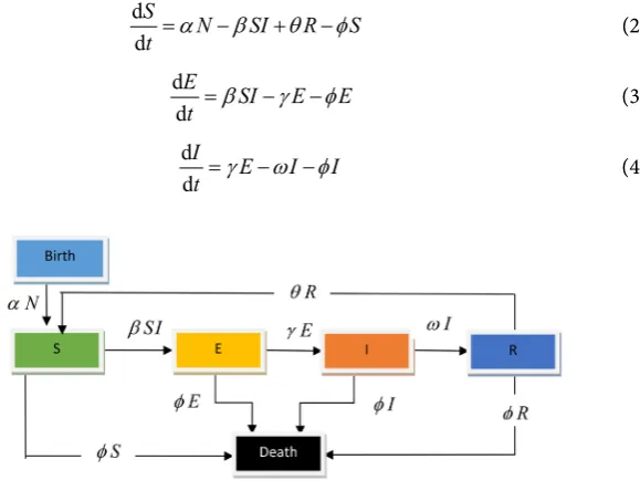
Newly born population merge into the S compartment at the rate of alpha (α), which represents the birth rate. The infected population are those individ-uals who can contract the disease. However for the SEIR model, we also consider the exposed population that is those individuals who have the disease but are not yet infectious. After treatment the infected population will move into R-Com- partment, at the rate of omega ω i.e. the recovery rate. Cattles can lose their immunity after some time. Let us assume a rate of
θ
. As a result, that popula-tion moves from R into the S compartment. Hence the following S-E-I-R-S Epi-demiological model without control is shown in Figure 1 as:DOI: 10.4236/aid.2019.91002 10 Advances in Infectious Diseases characterized by the following assumptions
• The population is homogeneous.
• No demographics,(immigration and emigration) consideration
• Birth rate and natural death rate are constant. Mathematically this means
( )
( ) ( )
( )
S t +E t +I t +R t =N (1)
where N is the total population. This facilitates the expression of one of the va-riables in terms of the others and the conserved constant N. Table 1 shows the description of the model parameters and variables applied in this study.
d d
S N SI R S
t =α −β +θ −φ (2) d
d
E SI E E
t =β −γ −φ (3) d
d
I E I I
[image:3.595.245.535.206.428.2]t =γ −ω −φ (4)
Figure 1. SEIRS Model without Control.
Table 1. Descriptions for variables for the model.
No. parameter Description
1 N Total population
2 S Susceptible to be expose for infection those of who interact with the disease 3 E Exposed population that are infected but have not yet become infectious
4 I Infected by the disease who are capable of transmitting the disease to any susceptible individuals.
5 R who are temporarily immune from the infection Individuals recovered from infection
6 α Birth rate from the total population N
7 β The rate of population exposed to the disease.
8 γ The rate which will be infected from the population of exposed
9 ω The rate of getting immunity after sort of treatment
in move to the recovered compartment from infected compartment.
10 θ The rate of populations loss their immunity and moved to the susceptible compartment.
[image:3.595.189.532.472.745.2]DOI: 10.4236/aid.2019.91002 11 Advances in Infectious Diseases d
d
R I R R
t =ω −θ −φ (5) Note that the natural death rate on each of the compartment for this paper is the same, which is
(
)
S E I R S E I R N
φ +φ +φ +φ =φ + + + =φ (6)
3. Optimal Control
Optimal control deals with the problem of finding a control law for a given sys-tem such that a certain optimal criterion is achieved. A control problem includes a function of state and control variable. An optimal control is a set of differential equations describing the paths of the control variables that minimize the cost function. The control can be derived using Pontryagins maximum principles (a necessary condition also known as Pontryagins minimum principle or simply Pontryagins Principle), or by solving the Hamilton-Jacobi-Bellamn Equations (a sufficient condition), [13]. This boundary-value problem actually has a special structure because it arises from taking the derivative of a Hamiltonian. Thus, the resulting dynamical system is a Hamiltonian system of the form
H x
λ ∂ =
∂
(7) H
x λ= −∂
∂
(8)
where
T T
H L= +λ a−µ b (9)
is an augmented Hamiltonian [14]. For this study, vaccination is applied as an optimal control and is denoted as u.
Numerical Solutions of Optimal Control Problems
Consider the optimal control problem( ) ( )
(
)
1
0
max t , , d
t
U f t x t u t
∫
t (10)( ) ( )
(
)
subject to : x′ =g t x t u t, , (11)
( )
0 0,( )
1 freex t =x x t (12)
Any solution to the above optimal control problem must also satisfy
( )
(
,( ) ( )
,)
,( )
0 0x t′ =g t x t u t x t =x (13)
( )
t Hx(
f t x ux(
, ,) ( ) (
t g t x ux , ,)
)
,( )
t1 0 δλ λ λ
δ
= − = − + = (14)
(
) ( ) (
)
(
)
*0 Hx f t x u, , t g t x uu , , , atu
δ λ
δ
= = − + (15)
re-DOI: 10.4236/aid.2019.91002 12 Advances in Infectious Diseases presentation of u* in terms of t, x, and
λ
.An optimal control with bounded control can be written in the form
( ) ( )
(
)
(
( ) ( )
)
0
max , tf , , d
uJ x t u =
∫
t f t x t u t t (16)Subject to
( ) ( )
(
)
( )
( )
0 0 , ,x g t x t u t
x t x
a u t b
′ = < ≤ ≤ (17)
where a, b are fixed real constants and a < b.
Proposition (Necessary conditions):- If u t*
( )
and x t*( )
are optimal for Equations (16, 17), then there exists a piecewise differentiable adjoint variable( )
tλ such that
( ) ( ) ( )
(
, * , ,)
(
,( ) ( ) ( )
, * ,)
H t x t u t λ t ≤H t x t u t λ t (18)
For all controls u at each time t, where H is the Hamiltonian, [13].
( )
t H x t u t(
*( ) ( ) ( )
, * , t)
x
δ λ
λ
δ
′ = − (adjoint condition) (19)
( )
ft 0λ = (transversality condition) (20)
By an adaptation of the Pontryagin’s Maximum Principle (PMP), the OC must satisfy (optimal condition):
*
if 0,
, if 0,
, if 0,
H a
u
H H
u a b
u u H H b a u u δ δ δ δ δ δ δ δ δ δ <
= < < =
< < >
(21)
If we have a minimization problem, then u* is chosen to minimize H point wise.
If 2H2 0 u ∂ <
∂ at
*
u then u is the maximization of the problem, while 2 2 0 H u ∂ <
∂ goes with minimization. The optimal control H 0
u δ
δ = obtained without truncation, and is bounded by a and b such that:
( )
* min ,max , H
u t a b
u δ δ =
(22)
Runge-Kutta (RK4) routine is applied for the numerical solution. It is re-quired that:
( )
( )
1
n
old
i= u i u i
−
DOI: 10.4236/aid.2019.91002 13 Advances in Infectious Diseases
old u u
u δ
−
≤ (23)
where
δ
is the accepted tolerance? The optimal control problem can now be written in a standard form:( )
( )
1
2
0
max
∫
Ax t −Bu t td (24)Subject to:-
( )
1 2( )
( )
2x t′ = − x t Cu t+ (25)
( )
0 0 fixed( )
1 freex =x x
In order for this to be a maximization problem, we require B > 0. The Hamil-tonian given by
2 1 2
H Ax Bu= − − +C uλ (26)
By applying the optimal condition
*
0 2
2
H Bu C u C
u B
δ λ λ
δ
= = − + ⇒ = (27)
( )
2( )
0
1 , 0
2
x t′ = − x +Cu x =x (28)
( )
t A x ,( )
1 0λ′ = − + λ λ = (29)
The Runge-Kutta forward sweep yields the transient profile of the dependent variable. The new u* is calculated by setting
1 2
u C
B λ = ∗
∗ (30)
(
1)
0.5 old
u= ∗ u u+ (31)
4. ODE Formulation for Optimal Control
4.1. Modification of SEIRS Model
A typical optimal control problem requires a performance index or cost function
( ) ( )
(
J x t u t , )
, a set of state variables(
x t( )
∈X)
and a set of control va-riables(
u t( )
∈U)
in a time t, t0 ≤ ≤t tf. A major goal of the work reportedherein, is to find a piecewise continuous control u(t) (vaccination) and the asso-ciated state variable x(t) to minimize a given objective functional. This strategy will directly impact on the susceptible “S” and the recovered “R” compartments in the overall mathematical formulation as shown below.
(
1)
2d 1
d
S v N SI v S R S
t =α − −β − +θ −φ (32) d
d
E SI E E
t =β −γ −φ (33) d
d
I E I I
DOI: 10.4236/aid.2019.91002 14 Advances in Infectious Diseases
1 2
d d
R v N v S I R R
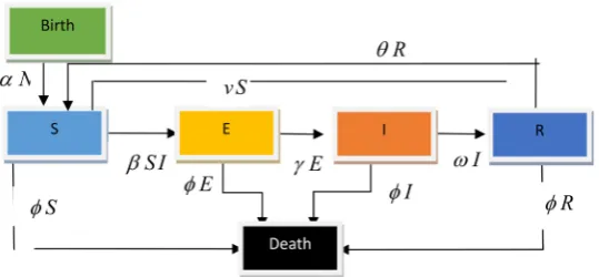
t =α + +ω −θ −φ (35) In the above equations, vaccination is applied during g birth v1, and for pop-ulations in the S-compartment v2, thus vaccinated populations moved to re-covered compartment as αv N1 and v S2 . However, for this paper, we applied vaccination on S-compartment only as (vS), and the formulation is given as below.
d d
S N SI vS R S
t =α −β − +θ −φ (36) d
d
E SI E E
t =β −γ −φ (37) d
d
I E I I
t =γ −ω −φ (38) d
dR vS I R Rt = +ω −θ −φ (39) With initial conditions,
( )
( )
( )
00( )
000 0, 0 0
0 0, 0 0
S S E E
I I R R
= ≥ = ≥
= ≥ = ≥
The above equations are illustrated graphically in Figure 2 as:
The optimal problem (which is the main objectives of this paper) is to minim-ize the objective (cost) functional (J) by considering the costs of vaccination for susceptible population given by:
( )
20
1 d
2
t
J u = AI+ Bu t
∫
(40)where:-
t: represents the vaccination period
A: a parameter that balancing cost factors due to the size of ineffective B: represents the weight attached on the cost of vaccination
A and B can also be weight parameters describing the comparative importance of the two terms (disease burden and cost) in the functional respectively.
A high value of A means that it is more important to reduce the disease bur-den than to reduce the vaccination costs. A less value of B means that it is more important to reduce the vaccination costs than to reduce the disease burden. The control u is the percentage of the susceptible that is vaccinated per unit time. Thus, u lies between 0 and 1 while umax will depend on the amount of resources
available to implement each of the control measures.
If u = 0, then no vaccination is done which is uncontrolled. If u = 1, then all susceptible population is vaccinated.
The rate of vaccination is assumed to take values in [0, 0.9] instead of [0, 1] to eliminate the case where the entire susceptible population is vaccinated.
DOI: 10.4236/aid.2019.91002 15 Advances in Infectious Diseases
Figure 2. Optimal control with vaccination.
Hence, the Optimal Control problem of the nonlinear dynamics of SEIRS LSD epidemic model studied herein is given by;
( )
20 1
min min d
2
t
uJ u = AI+ Bu t
∫
(41)where U u t=
( )
: 0≤ ≤u umax <1,t∈[ ]
0,t .For the Hamiltonian function:
(
)
(
)
(
)
(
)
1 2 3 4 4
1
1 2 3 4
, , , , , , , ,
, , , , , , , , , , , ,
d d d d
, , , , , ,
d d d d
i i i H t S E I R
f t S E I R u v g t S E I R u v
S E I R
f t S E I R u v
t t t t
λ λ λ λ
λ
λ λ λ λ
=
= +
= + + + +
∑
(42)Then by substituting each of the derivatives in Equation (41) into Equation (42) and by applying PMP to the Hamiltonian, we have:
(
)
(
)
(
)
(
)
2 1 2 3 4 1 2H AI Bu N SI uS R S
SI E E E I I
uS I R R
λ α β θ φ
λ β γ φ λ γ ω φ
λ ω θ φ
= + + − − + − + − − + − − + + − − (43)
The Adjoint functions with respect to the dependent variables are: For S:
(
)
(
)
* 1
*
1 1 2 4
*
1 1 2 4
H S
I u I u
I u I u
δ λ
δ
λ λ β φ λ β λ
λ λ β φ λ β λ
= −
⇒ = − − − + +
⇒ = − + + − −
(44)
Adjoint function with respect to E
(
)
(
)
* 2
*
2 2 3
*
2 2 3
H E δ λ
δ
λ λ γ φ λ γ
λ λ γ φ λ γ
= −
⇒ = − − − +
⇒ = + −
(45)
DOI: 10.4236/aid.2019.91002 16 Advances in Infectious Diseases
(
)
(
)
(
)
* 3 *3 1 2 3 4
*
3 1 2 3 4
H I
A S S
A S S
δ λ
δ
λ λ β λ β λ φ ω λ ω
λ λ β λ β λ φ ω λ ω
= −
⇒ = − + − + + − − +
⇒ = − + − + + −
(46)
Adjoint function with respect to R
( )
(
)
(
)
* 4
*
4 1 4
*
4 1 4
H R δ λ
δ
λ λ θ λ θ φ
λ λ θ λ θ φ
= −
⇒ = − + − −
⇒ = − + +
(47)
From the Equation (43 to 47); we obtain:
(
)
(
)
(
)
(
)
*
1 1 2 4
*
2 2 3
*
3 1 2 3 4
*
4 1 4
I u I u
A S S
λ λ β φ λ β λ
λ λ γ φ λ γ
λ λ β λ β λ φ ω λ ω
λ λ θ λ θ φ
= − + + − −
= + −
= − + − + + −
= − + +
(48)
With transversality conditions we have λi
( )
T =0,i=1,2,3,4Next, we consider an optimal condition for determining the characterization of the optimal control u*. The optimal condition by differentiating the Hamil-tonian H with respect to u based on the Equation (27) for each control u*. We have the following optimal system:
0 H
u δ
δ = at u u= * ⇒Bu+λ1
( )
−S , at u u= *then we have *
( )
1S u tB λ
= taking into account the bound u* and its characte-rization obtain;
* 1
0 if 0,
if 0,
0.9 if 0
H u S H u B u H u δ δ δ λ δ δ δ < = = > (49)
the optimal control u* can now be put in a compact form: *
1
max min S,0.9 ,0 u B λ =
(50)
Hence using the characterization of the optimal control, we now have follow-ing optimal system
S N SI uS R S
E SI E E
I E I I
R uS I R R
α β θ φ
β γ φ
γ ω φ
ω θ φ
′ = − − + −
′ = − −
′ = − −
′ = + − −
(51)
( )
0 0 0,( )
0 0 0, 0( )
0 0, 0( )
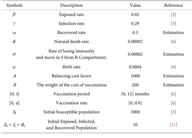
0 0DOI: 10.4236/aid.2019.91002 17 Advances in Infectious Diseases To determine the optimal vaccination, we use a forward-backward sweep nu-merical method. The model solves the SEIRS Equations (36 to 39) using fourth order Runge-Kutta (RK4) method. The values of all the accompanying parame-ters necessary for the successful numerical solution of the governing equations are given in Table 2
.
4.2. Numerical Results and Discussion
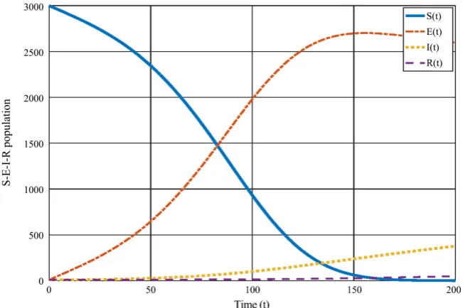
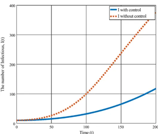
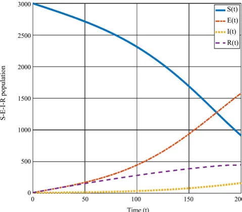
In Figure 3, no optimal control was applied. The number of populations in S is dramatically decreased. Whereas the number of Exposed populations exhibits an increase with time (t). After some time, the population shows an increase in E-compartment. As time progresses, the number of population in I compart-ment increases, while the number of population in R-decrease. This suggests an endemic situation.
[image:10.595.207.538.493.732.2]Unlike the previous case, Figure 4 displays the effect of optimal control (vac-cination) on the susceptible population. As a consequence of vaccination, there is a movement of the vaccinated population from the S compartment to the re-covery compartment. This is confirmed by an increase in the rere-covery popula-tion in the graph. We hasten to comment that irrespective of any control strate-gy, the population in the S compartment displays a decline as time progresses, but the rate of decrease when vaccination is applied is slower. With the popula-tion in the S-compartment vaccinated, recovery is enhanced. This shows that LSD disease can be controlled with vaccination. In addition, Figure 4 displays the response of the population in the S-compartment, for optimal control and non optimal control applications. For both cases, the size of the population de-creases at different rates. The profiles for both cases clearly demonstrate the ef-fect of the application of this treatment strategy for the susceptible population.
Table 2. Assigned values for model parameters.
Symbols Description Value Reference
β Exposed rate 0.02 [2]
γ Infection rate 0.29 [3]
ω Recovered rate 0.3 Estimation
φ Natural death rate 0.00002 [6]
θ Rate of losing immunity
and move to S from R Compartment. 0.00002 Estimation
α Birth rate 0.0004 [6]
A Balancing cost factor 1000 Estimation
B The weight of the cost of vaccination 200 Estimation
[0, t] Vaccination period [0, 12] months [6]
[0, u] Vaccination rate [0, 0.9] [6]
S0 Initial Susceptible population 3000 [3]
DOI: 10.4236/aid.2019.91002 18 Advances in Infectious Diseases
[image:11.595.236.515.322.579.2]Figure 3. SEIRS without Optimal control.
Figure 4. S-compartment with optimal control and without optimal control.
DOI: 10.4236/aid.2019.91002 19 Advances in Infectious Diseases
[image:12.595.239.507.324.523.2]Figure 5. I-compartment with optimal control and without optimal control.
Figure 6. E-compartment with optimal control and without optimal control.
Figure 7 shows a dramatic rise in the “R” population resulting from the ap-plication of vaccination. This reflects an inflow from virtually all the compart-ments of the model into the “R” population when control is applied. This again shows that vaccination as intervention strategy has a great impact on controlling LSD among cattle.
For demonstration purposes, we present the effects of different vaccination rates
(
0≤ ≤ν 0.85)
on the SEIR profiles in order to assess the impact on the overall control strategy adopted for this study.DOI: 10.4236/aid.2019.91002 20 Advances in Infectious Diseases population decreases, they move to both the recovered (“R” population) and the exposed (the “E” i.e. the exposed or the latent population). There is a gradual rise in the “E” population as indicated in Figure 8. Initially it exhibits a higher profile than the “R” population (see Figure 9 and Figure 10). Figures 11-13 show that it finally catches up with and surpasses the exposed population. The actual point of transition happens around
ν
=0.6. Given the parameters adopted in this study this can be considered as an optimal point of application and the decision as to whether to continue increasing the vaccination rate will depend on other consideration among which will be that availability of funds. From Figures 8-13, it can also be observed that the profile of the infected popu-lation (the “I” compartment) remains the lowest when compared to the dynamic profiles exhibited by other compartments.Figure 7. R-compartment with OC and without OC.
[image:13.595.253.493.495.705.2]DOI: 10.4236/aid.2019.91002 21 Advances in Infectious Diseases
[image:14.595.244.500.302.475.2]Figure 9. SEIR-compartment with optimal control at u [0, 0.3].
Figure 10. SEIR-compartment with optimal control at u [0, 0.5].
[image:14.595.247.504.510.701.2]DOI: 10.4236/aid.2019.91002 22 Advances in Infectious Diseases
Figure 12. SEIR-Compartment with Optimal Control at u [0, 0.75].
Figure 13. SEIR-Compartment with Optimal Control at u [0, 0.85].
5. Conclusions
[image:15.595.236.513.343.553.2]DOI: 10.4236/aid.2019.91002 23 Advances in Infectious Diseases Both the controlled and uncontrolled scenarios were demonstrated graphical-ly in order to identify the optimal vaccination schedule for the treatment and assessment of the impact of LSD on the cattle population. The results of our numerical experiments (Figures 8-13) clearly demonstrate that the applied op-timality measures and intervention protocol have a very desirable effect in trolling and reducing the number of infected cattle population during the con-trol period as long as they are properly managed. In addition, as the concon-trol pe-riod increases the number of cattle population saved from LSD gradually in-creased.
Based on our LSD model and parameters adopted for this study, the effects of the optimal vaccination strategy can be assessed for the vaccination rates in the range of
(
0≤ ≤ν 0.85)
. It is observed that the control measures adopted herein achieves optimal operation at approximatelyν
=0.6.Conflicts of Interest
The authors declare no conflicts of interest regarding the publication of this pa-per.
References
[1] Abera, Z., Degefu, H., Gari, G. and Ayana, Z. (2015) Review on Epidemiology and Economic Importance of Lumpy Skin Disease. International Journal of Basic and Applied Virology, 4, 8-21.
[2] Birhanu, H. and Gezahign, A. (2015) Epidemiology, Economic Importance and Control Techniques of Lumpy Skin Disease: A Review. International Journal of Agricultural Research and Review, 3, 197-205.
[3] Regbe, H. (2012) Lumpy Skin Disease (LSD): Outbreak Investigation, Isolation and Molecular Detection of LSD in Selected Areas of Eastern Shewa, Ethiopia. Master Thesis, The School of Graduate Study of Addis Ababa University.
[4] Alaa, A., Hatem, M. and Khaled, A. (2008) Polymerase Chain Reaction for Rapid Diagnosis of a Recent Lumpy Skin Disease Virus Incursion to Egypt. Arab Journal of Biotechnology, 11, 293-302.
[5] Hawsar, Y.A., Heshu, S.R., Hiewa, O.D. and Hemn, H.O. (2016) Lumpy Skin Dis-ease. Reproductive Immunology, 1, 25.
[6] Birhanu, H., Gezahign, A. and Nuru, S. (2015) Techniques of Lumpy Skin Disease. Animal. https://doi.org/10.11648/j.avs.20150302.15
[7] Davies, G. (1991) Lumpy Skin Disease, an African Capripox Virus Disease of Cattle. The Veterinary Journal, 147, 489-502.
https://doi.org/10.1016/0007-1935(91)90019-J
[8] OIE (2010) OIE Manual of Diagnostic Tests and Vaccines for Terrestrial Animals. Lumpy Skin Disease, 14, 768-778.
[9] Tuppurainen, E.S.M. and Oura, C.A.L. (2012) Review: Lumpy Skin Disease: An Emerging Threat to Europe, the Middle East and Asia. Transboundary and Emerg-ing Diseases, 59, 4048. https://doi.org/10.1111/j.1865-1682.2011.01242.x
Epi-DOI: 10.4236/aid.2019.91002 24 Advances in Infectious Diseases demiology & Infection, 126, 317-321. https://doi.org/10.1017/S0950268801005179 [11] Gari, G., Waret-Szkuta, A., Grosbois, V., Jacquite, P. and Roger, F. (2010) Risk
Fac-tors Associated with Observed Clinical Lumpy Skin Disease in Ethiopia. Epidemi-ology & Infection, 138, 1657-1666. https://doi.org/10.1017/S0950268810000506 [12] Lenhart, S., Bodine, E., Zhong, P. and Joshi, H. (2013) Illustrating Optimal Control
Applications with Discrete and Continuous Features. Fields Institute Communica-tions, 66, 209-238. https://doi.org/10.1007/978-1-4614-5389-5_9
![Figure 9. SEIR-compartment with optimal control at u [0, 0.3].](https://thumb-us.123doks.com/thumbv2/123dok_us/9103316.407523/14.595.247.504.510.701/figure-seir-compartment-optimal-control-u.webp)
![Figure 12. SEIR-Compartment with Optimal Control at u [0, 0.75].](https://thumb-us.123doks.com/thumbv2/123dok_us/9103316.407523/15.595.236.513.343.553/figure-seir-compartment-optimal-control-u.webp)
