Error Free Training via Information Structuring in the Classification Problem

(1)

ISSN Online: 2150-8410 ISSN Print: 2150-8402

DOI: 10.4236/jilsa.2018.103005 Aug. 6, 2018 81 Journal of Intelligent Learning Systems and Applications

Error-Free Training via Information

Structuring in the Classification Problem

Vladimir N. Shats

*

St. Petersburg, Russia

Abstract

The present paper solves the training problem that comprises the initial phases of the classification problem using the data matrix invariant method. The method is reduced to an approximate “slicing” of the information con-tained in the problem, which leads to its structuring. According to this me-thod, the values of each feature are divided into an equal number of intervals, and lists of objects falling into these intervals are constructed. Objects are identified by a set of numbers of intervals, i.e., indices, for each feature. As-suming that the feature values within any interval are approximately the same, we calculate frequency features for objects of different classes that are equal to the frequencies of the corresponding indices. These features allow us to determine the frequency of any object class as the sum of the frequencies of the indices. For any number of intervals, the maximum frequency corres-ponds to a class object. If the features do not contain repeated values, the er-ror rate of training tends to zero for an infinite number of intervals. If this condition is not fulfilled, a preliminary randomization of the features should be carried out.

Keywords

Classification Algorithms, Granular Computing, Invariants of Matrix Data, Data Processing

1. Introduction

The classification problem addresses numerous questions in science and tech-nology that involve the use of massive amounts of accumulated information in analyses of new data. These data play the role of incoming information in vari-ous models of formalized complex systems. The accumulated information is represented by objects, and the features of objects are vectors, usually in

Eucli-*Independent researcher. How to cite this paper: Shats, V.N. (2018)

Error-Free Training via Information Struc-turing in the Classification Problem. Jour-nal of Intelligent Learning Systems and Applications, 10, 81-92.

https://doi.org/10.4236/jilsa.2018.103005

Received: May 15, 2018 Accepted: August 3, 2018 Published: August 6, 2018

http://creativecommons.org/licenses/by/4.0/

(2)

DOI: 10.4236/jilsa.2018.103005 82 Journal of Intelligent Learning Systems and Applications

dean space [1] [2] [3].

This representation of objects allows for the use of the powerful technique of linear algebra to study the properties of the corresponding samples. However, this method is based on a sufficiently strong assumption that does not take into account important features of the problem itself. In this problem, real objects are represented by information that describes quantitative images, patterns, and the values of randomly selected features include random errors derived from the measurements or observations. Uncertain data are organically inherent in such tasks relevant to the field of artificial intelligence, in which pragmatic informa-tion is processed. A specific task is posed by some expert who, guided by profes-sional expertise, classifies a set of real objects and describes their patterns that are obtained experimentally. Therefore, we here relate the sensory perception of a real object by an expert to the quantitative representation of that object. There clearly cannot be a one-to-one correspondence between the perception of the object and its measurement.

Furthermore, existing methods assume the existence of metric space features and a smooth probability density function for objects of a certain class. Howev-er, in a real problem, all objects have similar or identical feature values; thus, the object classes differ only in the probability densities of the features. However, only a generalized function can accurately consider the discontinuous densities of the features. Therefore, each of the existing methods is applied over a re-stricted area whose boundaries can usually only be established experimentally.

These considerations were taken into account when developing the data ma-trix invariant method for solving the classification problem [4] [5]. According to this method, a given data matrix is one possible random realization of the set of matrices describing the properties of a sample. This set is here considered to be a set of invariants with respect to the class of objects. The method is based on a concept presented by L. Zadeh. This concept states that the solution of most problems does not require high accuracy because humans perceive only “a trickle of information” from the external world [6]. Moreover, in systems in which complexity exceeds a certain threshold, accuracy and practical sense are almost mutually exclusive.

According to the method, solving the classification problem consists of two stages. In the “training phase” (following [1]), the method calculates a function that uses the simplest and most universal algorithm and establishes a rule ac-cording to which the training sample is divided into classes. In the second stage, this function is used to classify new objects.

(3)

classes. Her work, which reduces to the interactions among granules, manifests itself in the frequencies of their appearance.

2. Assumptions and Preliminary Observations

The solution is sought in accordance with the following algorithm. The range of values of each feature is divided into an equal number of intervals and the num-ber of each interval, called the index, in which the object feature falls is deter-mined. The objects are then described by a set of indices, and the data matrix is transformed into an index matrix. For each feature, it is possible to find a subset of objects with the same index and these subsets are referred to as granules. The frequency of a certain object’s classes can then be calculated in terms of the composition of the granules. The sum of the frequencies of the granules that correspond to individual features is approximately equal to the frequency of oc-currence of a certain class object. The maximum of this frequency gives an esti-mate of the object class for any number of intervals.

The proposed algorithm is conceptually based on the fact that the uncertain quantities are quantities that yield different quantitative information about a single entity. On this basis, the assumption is made here that the given values of the features are random and that values within a certain neighborhood are equally probable. According to this assumption, the probability distribution of features is piecewise constant. Therefore, each feature value of an object can be assigned an index, and for each class, the frequency of the teaching sample is calculated.

The probability of a particular object class consists of a complete group of in-dependent events of index appearance for all features in the same class. Then, the process of classification is reduced to a comparison of the frequencies of dif-ferent class objects whose feature indices have the frequencies of the corres-ponding classes. The formula of full probability allows estimating the probability of an object for each class, and its maximum defines an object class.

In general, the compositions of granules (in terms of their feature values and object class) are highly uncertain, and it is advisable to reduce this uncertainty to eliminate possible classification errors. This objective can be partly achieved by increasing the number of intervals to infinity when the granules are composed only of objects with the same feature values.

(4)

val-DOI: 10.4236/jilsa.2018.103005 84 Journal of Intelligent Learning Systems and Applications

ues by a uniformly distributed random variable that is the same for all features of the object. All of the features then have different meanings, and the training will be asymptotically error-free. An analysis of the solutions for a variety of training sample models shows that this conclusion is valid for any real problem.

The invariant method represents a model of processes in the sensory systems of animals and is intended to carry out class recognition by searching for proto-type objects in the information stored in an animal’s brain [9]. A single algo-rithm for implementing the method and model indicates the biological roots of the proposed approach and confirms its applicability.

3. Features of the New Multidimensional Data Description

System

3.1. Statement of the Problem

The basis of this work is the data matrix invariant method. This method allows the establishment of a function that divides the objects in a training sample into classes. The effectiveness of the method has been demonstrated using 9 databas-es from a repository [10]. These databases cover a wide range of values in terms of the numbers of objects, features, and classes; the types of features; and the unevenness of the distribution of objects between classes. This article focuses on the limits of the application of the method for the first stage of the solution and the refinement of some features of the method. To this end, we consider the fol-lowing training problem involving the application of models to sample data.

Let X=

{

x ss| ∈

(

1,M

)

}

be sample objects that describe feature vectors

(

)

T

1, ,

s s s

Mk

q q

=

q  . Additionally, Q is a data matrix; ωi is a list of numbers of

objects of class i∈

(

1,Mi

)

_; M Mi, and Mk are the number of objects, classes and attributes, respectively, and there are no missing data. In the task, it is ne-cessary to establish a function according to which objects are divided into classes and to assess the influence of various peculiarities of the data on the class recog-nition accuracy.

The properties of an object are determined by combining the values of its fea-tures, and it can naturally be assumed that objects of different classes differ only in the probability distribution of the features. Therefore, each data set is created by the methods of statistical modeling as the union of sets of individual class ob-jects with different feature densities. The values of each feature

{

1_{, ,} Mk

}

k k k

q ∈ q _ q

are generated by a mixture Mi of normal distributions

(

, ,i i

)

k k k

N q

µ σ

. Here,

0

i i

k k k

µ

=

µ µ

∗ and i 0i

k k k

σ

=

σ σ

∗ are the sample mean and sample standard deviation of the list of objects ωi, respectively, and M k, µ and k

σ

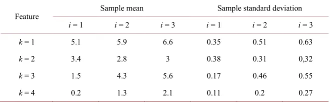
are model

parameters. The values of 0i k

µ

and 0i

k

σ

indicated in Table 1, where Mi=3 and Mk=4, correspond to the Iris database [10]. The distribution of objects by class (5%, 35% and 60%) indicates that the data are “unbalanced”, which com-plicates the classification problems [11].

(5)

[image:5.595.209.540.90.192.2]

Table 1. Parameters of the initial distribution of features.

Feature Sample mean Sample standard deviation

i = 1 i = 2 i = 3 i = 1 i = 2 i = 3

k = 1 5.1 5.9 6.6 0.35 0.51 0.63

k = 2 3.4 2.8 3 0.38 0.31 0,32

k = 3 1.5 4.3 5.6 0.17 0.46 0.55

k = 4 0.2 1.3 2.1 0.11 0.2 0.27

rounding error, several new samples whose data matrices differ importantly are generated. The variance in several features of one of the classes can be zero. For the features of individual classes and the data set as a whole, the correlation de-pendence varies widely, from very strong to very weak and from positive to neg-ative.

The sample models are identified by the character string a_b_c, where a and b are the values of kµ and k

σ

_{, respectively, and}_c_{is the rounding parameter.} For c, the values of 0, 1, 2 and 3 correspond to the rounding up of integers, tenths, hundredths and no rounding, respectively. The conclusions obtained in the work are based on an analysis of a large volume of calculated data, the cha-racteristic features of which are illustrated in the figures cited in the paper.

Within the framework of the method, we consider the vector of object features to be an ordered set of feature values to which the segments of the coordinate axes correspond. The object itself is considered to represent a certain point in the multidimensional coordinate system. The totality of such points for all sam-pling objects determines the feature space. This space is not Euclidean, as is cus-tomary in machine learning, because the additional assumption of the existence of the scalar product is not made. Here, we use only the structure of the space, the points of which differ in terms of their numbers and related information.

3.2. Multidimensional Intervals

Let us divide the objects into groups in which the values of each feature lie close to one another. For this purpose, we use multidimensional intervals that break the range of values of each feature into an equal number of intervals. For any k, we then obtain the intervals of values qk∈qk m, ,qk m, + ∆k

)

with the step

(

max min

)

(

₁

)

k qk qk n

∆ = − − _{, where} n>1_{is the number of intervals;} m∈

( )

1,n is the interval number; and min

k

q and max k

q are the minimum and maximum values of the feature, respectively. We call m the feature’s index k of the object s if qks∈ qk m, ,qk m, 1+

)

.

There are two variants of indexation and of the corresponding function

: s k

q m

ϕ

→ _{. The first variant realizes the dependence} 1 ks kmin k q q

m= + W −_∆ 

 ,

where the function W

( )

⋅ _{calculates the integer part of the number.} The second option assumes that s

k

(6)

such that the value t k

q is arranged in nondecreasing order: 1 2 M

k k k

q ≤q ≤_≤q _.

The index m = 1 receives one or several objects (with numbers t) for which

)

, , , t

k k m k m k

q ∈_q q + ∆ _{, where} min ,

k m k

q =q _{. If, with a further increase in}_t_{, this} re-lation is not satisfied for some t t= 1, we then take m m= +1 and qk m, =qtk1

and find the group of objects for which m = 2. In the same way, we successively determine the indices of all other values of the features.

The indices computed in accordance with options 1 and 2 (hereinafter indices i1 and i2) may differ significantly. For example, under M = 100 and n = 1000, the values of i1 1,1000∈

[

]

_{, and they are described by 100 different numbers,} while the values of i2 1,31∈

[ ]

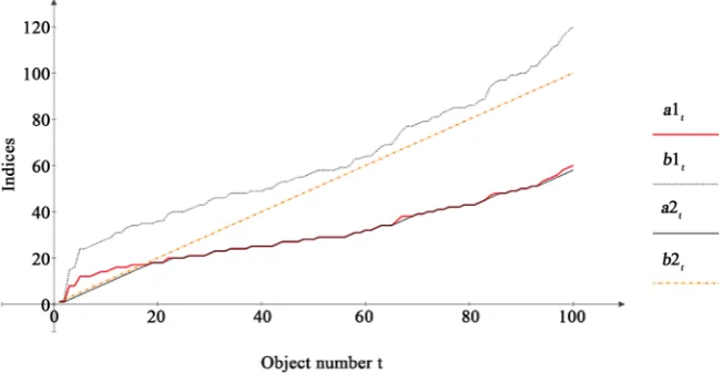
_{, and some numbers are repeated many times. The} correlation coefficients of the feature vectors and their indices are equal to 1 for i1 and close to 1 for i2.

The curves in Figure 1 illustrate the effects of the parameter n on the index values for the feature vector with M = 100 distributed according to the normal law. (For clarity, the curves are plotted for no decreasing feature values). The curves a1 and b1 correspond to the index i1 when n = 70 and 120, respectively, while similar curves a2 and b2 exist for index i2. Here and in the other figures, the identifiers of the curves are supplemented with identifiers of the variants of the indices. The graphs show that the indices i1 and i2 almost coincide for n < M and differ significantly for n > M.

3.3. Granulation of the Given Data

[image:6.595.211.538.533.702.2]

Given the uncertainty of the data, we introduce the assumption that all of the values of the features of the objects fall within a certain interval and include some random errors that are equal. For each indexing option, we find the data matrix mapping Q→D. Here, D=

( )

ds k, is the index matrix, and ds k, is the index feature k of the object s. The matrix

D

has an important feature. Its elements do not characterize the meanings of the features of the objects; instead, these elements indicate the “locations” of their values in the structure of the ma-trix Q. If we were to represent some feature value of the object in the form of a

(7)

particle, it would be located in the element of the matrix

D

that corresponds to the index for this feature.

The matrix

D

makes it easy to find subsets of objects Zk m, that have the same values of the ordered pair

(

,

)

( )

, s

k

k m = k d _{for any}_k_and_m_{. We call} Z_{k m}_, the information granule.

Let lk m, be the number of objects in the granule Zk m, , among which lk mi, have class i. Thus, the frequency of objects in class i in this granule is

, , ,

i i

k m k m k m

g =l l . According to the accepted assumption, any object of class i in the granule Zk m, has the frequency gik m, and therefore the sample probability

(

i| ks

)

k mi,

p s∈

ω

d =m =g _.

The event occurrence of vector _ds_{for objects of class}_i_{consists of the}

com-plete group of independent events d1s, , dMks . It follows from the total

proba-bility formula that the probaproba-bility estimate for this event is

(

)

1 , ,

1

| s Mk i i

i k k m k m

p s g g

Mk

ω

₌

∈ d d= =

∑

= (1)

Here, gk mi, is the average frequency gk mi, for all k. The calculated class of object s corresponds to the maximum of this value for a given n:

(

)

1

arg max | s

n i Mi i

I = ≤ ≤ p s∈

ω

d d= (2)

This formula establishes a rule for recognizing an object class as a result of training using the sample data. According to (2), the object class depends on the frequency gk mi, , which serves as an objective measure of the membership of any object from the set X to a certain class based on separate features. The evaluation of the class is robust because the grouping of objects is performed in its calcula-tion. This operation neutralizes the influence of sharply differing feature values.

The accuracy of solving the training problem is determined by examining the fulfillment of the relation

( )

s

n

I s =i for each sample object. It is estimated by the frequency γn, which is equal to the ratio of the total number of errors to the

length of the sample.

3.4. Influence of the Parameter

n

We are interested in the properties of the sequence

{ }

γ

n where n=2,3,.

For some k, let the granule Zk m, contain an object s of class i, as well as other objects, including the object w. Therefore, in any scheme, indexing is performed following the inequality 0 w s

k k k

q q

≤ − ≤ ∆ _.

Consider the limiting case of n→ ∞ corresponding to the step ∆ →k 0. It

follows from the above relation that w s

k k

q =q . Since all of the values of the fea-ture are different in statistical modeling and in the absence of rounding, this equality is satisfied only when w s= _{. The granule} Z_{k m}_, then consists of a sin-gle object s having class i, and the frequency gk mi, =1 for any k∈

(

1,Mk

)

. Hence,

( )

s

n

I s →i for all s∈

(

1,M

)

, and the sequence

{ }

γ

n converges in

probability to zero.

(8)

calculates the class of any object of the training sample.

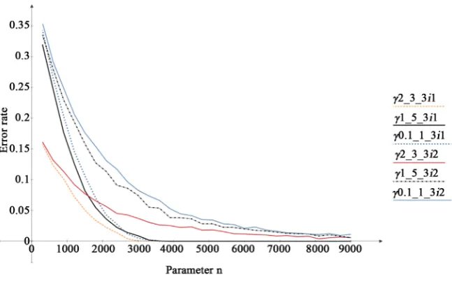
The results of calculations of the function f n

( )

=

γ

n for several samples ata

value of n = 3000 are illustrated by the curves shown in Figure 2. For all of the curves, a notation system is adopted in which the symbol γ is followed by a string of characters that act as the identifier of the sample, and the indexing op-tion i1 or i2 is then indicated. The graphs depict the sequence convergence process

{ }

γ

n . They show that the convergence rate for index i1 is higher than

that for i2.

The calculations show that the correlation coefficients of the features of indi-vidual classes and the corresponding indices i1 and i2 do not differ significantly.

3.5. Randomization of the Data

The question of the limitations of the given data in solving the training problem using the method considered naturally arises. In connection, we note that the curves in Figure 2 are plotted for the samples in which all of the features have different values, as obtained directly by statistical modeling (for c = 3). In real machine learning tasks, objects often have repeated, identical values. This situa-tion is not uncommon in the case of quantitative traits and is common in prob-lems in which traits are not examined quantitatively, but are represented by, for example, nominal and ordinal features. Here, this situation is modeled by rounding the feature values because the number of different feature values in the matrix Q can be significantly reduced by rounding. For example, if the value of c is decreased from 3 to 0 in sample 1_0.1_3, all of the values of q2 will be equal to 3.

The effect of rounding on the accuracy of training occurs via following me-chanism. Consider a granule Gk m, containing an object s of class i for some k in the case in which n→ ∞_{. Suppose that there is a set of objects}

{

w w₁, ,₂

}

of different classes in which w1 w2 s

k k k

[image:8.595.212.536.505.708.2]

q =q ==q . For any other k, a similar ratio

(9)

can be constructed. However, it will concern an analogous set made up entirely or partially of other objects because two objects with the same characteristics cannot exist in the sample. All of the summands that determine the value of

, i k m

g for the object s will be greater than zero. Since Mn, most of the ana-logous summands for the objects of the indicated sets will differ from zero only for some values of k and i. Therefore, given repeated values of the attributes, training errors occur.

Figure 3 shows the results of calculations for the three samples before and af-ter rounding to the nearest tenth (c = 3 and 1) for M = 200 and index i2. This figure shows that rounding leads to significant changes. A sequence

{ }

γ

n does

not converge in probability to zero; for sufficiently large values of n, there are portions with constant values γn.

This situation is explained by the fact that rounding changes the level of di-versity in the data β _{, which is equal to the average number of different feature} values in the sample. For example, for the sample 2_3_2 with M = 1000, a se-quence of values c=

{

3,2,1,0

}

_{corresponds to}

β

=

{

1000,478,87,11

}

_.

Accord-ing to the theory of K. Shannon, the amount of information per one feature val-ue increases proportionally to log 1000 log2

(

)

2

( )

β

. In this case, this volume changes in the ratio 1:1.12 :1.55: 2.88. The corresponding increase in “infor-mation overload” leads to a situation in which, for some objects, the values gk mi, will be the same for different i given a sufficiently large n. Formula (2) will then not be able to correctly predict the class of objects.

To avoid such errors, we use the idea of invariants and move from the data matrix to its invariant, in which features do not have repeating values. The inva-riant of the data matrix is found by randomization according to the assumption that, for all k∈

(

1,Mk

)

_and s∈

(

1,M

)

_{, we can replace} s

k q by s

k s

q +

α

v _{, where} v is a random variable uniformly distributed on the segment

[ ]

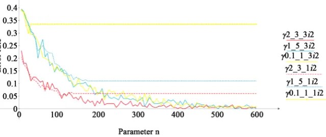
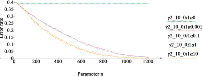
0,1 and α≥0 is a constant. Since the average values of each feature increase by α 2_{with this}

[image:9.595.216.536.569.703.2]

transformation, the correlation dependence of the features will not change. The influence of the parameter α on the training accuracy is shown in the curves given in Figure 4. The curves represent the results of calculations for the sample 2_10_0 with M = 1000, the index i1 and the five values α = 0, 0.001,

(10)

[image:10.595.213.538.78.202.2]

Figure 4. The impact of randomization on the accuracy of training.

0.1, 1 and 10. The curves show that the randomization effect occurs for any 0

α> . Since the values of the features are located on the segment [−7, 29], ran-domization results in significant relative changes for some of these values. How-ever, for all values of α, high-quality training is achieved; for these data sets, the influence of the parameter α is reflected only in the rate of convergence.

Thus, due to randomization, we cannot completely neutralize the effects of low levels of diversity and achieve error-free training.

3.6. Limitations of the Given Data

In the initial stage of sample modeling, the objects of each class differed in the distribution of their features. Rounding violated this provision as columns of the data matrix ceased to represent the calculated distribution. Nevertheless, for all of the samples, error-free training was achieved. Below, we consider the question of whether error-free training will be achieved for any sample.

Earlier, we examined samples that have equal values for some of the features and showed that the application of randomization enables the achievement of error-free training. It follows from computational experience that the case in which a relatively large number of objects have the same feature values requires special consideration.

Let each value p of the feature occur rp times and p∈

( )

1, ,l l M≤ . In this

case, the number of variants of the placement of the feature values is

1 2

!

! ! l!

M K

r r r

=

∗ ∗ ∗_

where 1 l

p

p= r =M

∑

[12]. For l M= , we obtain the limiting case in which all of the feature values differ from each other, for which r r1= =2 =rM =1 and

1 !

K =M _.

If only v of M objects have different feature values, then r v1= and

1 2 1

v v M

r+ =r+ ==r = . The number of variants is then equal to K2 =M_v_!!, and

(11)

information and is not actually taken into account, although it is “claimed” to be one of the features. It is thus a “degenerate” feature.

From the above dependences, it follows that the level of decrease in the en-tropy of the feature and the information it contains depends on the ratio of M to v. If M = 100, then the maximum value of the entropy is log 100! 3632

(

)

= bits due to the decrease in the repeated values of the features. Furthermore, for the sequence of values v=

{

70,90,99

}

_{, there will accordingly be 133, 45, 4.6 bits.}

As noted in the Introduction, the training problem, which is a stage of classi-fication, is formulated by an expert. Only this expert can decide whether a ma-trix carrying a limited amount of information can serve as a data mama-trix. For us, only the case v M= _{is obvious. In this case, the “degenerate” feature will}

re-ceive random information during the randomization stage, possibly distorting the essence of the problem.

A similar situation occurs if the sample variance for the entire sample or one class (for example, sample 10_0.1_3) is close to zero. Most of the values of this attribute will then be concentrated near the mathematical expectation, and it may turn out that all of the other values are represented by an extremely limited number of indices. Note also that an uneven distribution of objects by class can enhance the effect of reducing the volume of information. In such cases, the se-quence

{ }

γ

n cannot converge to zero. If the resulting error is significant, the

scheme for computing the invariants of the data matrix should then be changed by first converting the values of the corresponding feature. A similar transfor-mation for the Adult database led to error-free training [5].

For real datasets, we can assume that the invariant method leads to practically error-free training.

4. Conclusions

This paper presents a solution to the problem of training sample models by em-ploying the data matrix invariant method, which was developed to solve the classification problem. This solution is limited to finding a function according to that the objects in a training sample are divided into classes, studying the influ-ence of various data features on the accuracy of training.

The key idea of the method is structuring the information contained in the problem by introducing multidimensional intervals that allow us to roughly break up the given dataset into its component parts and to compute the infor-mation granules for each feature. The granules possess an important property in that, given an infinite number of interval; each granule contains only the objects with the same feature value.

(12)

Therefore, multidimensional intervals allow us to compare objects in a probabil-ity space, and they play the role of the concept of distance in determining the positions of objects in Euclidean space. The advantage is that the evaluation of the probability of an object is incomparably closer to solving a problem than evaluating the position of an object in a metric space.

In this paper, it is shown that the data matrix invariant method yields practically error-free training for any data matrix on the basis of a simple and universal algo-rithm. This method has independent importance because it offers a new way of analyzing multidimensional data that do not rely on the concept of distance be-tween objects.

Conflicts of Interest

The authors declare no conflicts of interest regarding the publication of this paper.

References

[1] Bishop, C. (2006) Pattern Recognition and Machine Learning. Springer, Berlin, 738. [2] Hastie, T., Tibshirani, R. and Friedman, J. (2009) The Elements of Statistical

Learn-ing: Data Mining, Inference, and Prediction. 2nd Edition, Springer, Berlin, 764.

https://doi.org/10.1007/978-0-387-84858-7

[3] Murphy, K. (2012) Machine Learning. A Probabilistic Perspective. MIT Press, Cambridge, Massachusetts, London, 1098.

[4] Shats, V.N. (2016) Invariants of Matrix Data in the Classification Problem. Stochas-tic Optimization in InformaStochas-tics, 12, 17-32.

[5] Shats, V.N. (2017) Classification Based on Invariants of the Data Matrix. Journal of Intelligent Learning Systems and Applications, 9, 35-46.

https://doi.org/10.4236/jilsa.2017.93004

[6] Zadeh, L. (1979) Fuzzy Sets and Information Granularity. In: Gupta, N., Ragade, R. and Yager, R., Eds., Advances in Fuzzy Set Theory and Applications, World Science Publishing, Amsterdam, 3-18.

[7] Yao, J., Vasiliacos, V. and Pedrycz, W. (2013) Granular Computing: Perspective and Challenges. IEEE Transactions on Cybernetics, 43, 1977-1989.

https://doi.org/10.1109/TSMCC.2012.2236648

[8] Ashby, W.R. (1957) An Introduction to Cybernetics. 2nd Edition, Chapman and Hall, London, 294.

[9] Shats, V.N. (2018) The Classification of Objects Based on a Model of Perception. In: Kryzhanovsky, B., Dunin-Barkowski, W. and Redko, V., Eds., Advances in Neural Computation, Machine Learning, and Cognitive Research, Studies in Computation-al Intelligence, Springer, Cham, 3-8. https://doi.org/10.1007/978-3-319-66604-4_1

[10] Asuncion, A. and Newman, D.J. (2007) UCI Machine Learning Repository. Irvine University of California, Irvine.

[11] Lopez, V., Fernandez, A., Garcia, S., Palade V. and Herrera F. (2013) An Insight in-to Classification with Imbalanced Data: Empirical Results and Current Trends on Using Data Intrinsic Characteristics. Information Sciences, 250, 113-141.

https://doi.org/10.1016/j.ins.2013.07.007