Accelerating the Search for
Optimal Dynamic Traffic Management
improving the Pareto optimal set of
Dynamic Traffic Management measures that
minimise externalities using function approximations
Accelerating the Search for
Optimal
Dynamic
Traffic
Management
improving the Pareto optimal set of Dynamic Traffic
Management measures that minimise externalities using
function approximations
Kornelis Fikse
Enschede, 3rd January 2011
In fulfilment of the Master Degree
Civil Engineering & Management, University of Twente, The Netherlands
Graduation Committee
Prof. dr. ir. E.C. van Berkum
Dr. T. Thomas
Dr. M.C.J. Bliemer
Summary
I don’t think many people have ever read the report [. . . ] How many read the summary?
John Sherman Cooper (1901 – 1991)
In the past decades traffic demand has been increasing nearly continuously, which has provided governments all over the world with significant challenges. In the Netherlands constructing new roads is, due to various reasons, not longer considered to be the solution, the focus is now more on efficient use of existing infrastructure.
One of the instruments that is frequently used to increase the efficiency of infrastructure is Dynamic Traffic Management (DTM). In DTM we use different measures such as directing traffic through traffic lights, adding or removing lanes and variable speed limits to provide road users with the ‘best possible’ infrastructure. It is however difficult to determine what is ‘best’, especially now environmental and safety issues are becoming more and more important. The best possible set of measures from a travel time perspective, may very well result in very high CO2 emissions, annoyance due to excessive
noise and many fatalities.
It is therefore that research is being done on determining a set of possible DTM applications that can be considered the best solutions. Here ‘best’ means that these solutions are not outperformed by any other solution on all objectives. Unfortunately finding all solutions in this set is impossible, it would easily take millennia to find them. Science has therefore resorted to finding only a part of this set (but a representative one) using heuristics such as Genetic Algorithms. However finding a part of this set using this method still takes months, which is unacceptable in the traffic and transport consultancy business. It is here where our research takes off.
Main goal of our research is therefore to accelerate the search for this set of best solutions (also known as Pareto optimal set). In our research we focus
solely on accelerations that can be obtained by using approximation tech-niques, which is why our research goal is defined as ‘accelerating the search for the Pareto optimal set found by multiobjective genetic algorithms for mul-tiobjective network design problems, in which externalities are the objectives and DTM measures the decision variables, using function approximations’.
It is therefore that we performed a literature study into approximation tech-niques, from which we derived three main techniques: the Response Surface Method (RSM), the Radial Basis Function (RBF) and Kriging/DACE. Be-cause all of the approximation techniques have parameters that can be set, we were able to develop 148 different variants. In order to be able to determine which variant would provide the best results, we chose two simple road net-works which could be used for testing and selected a set of quality measures from literature.
We found that variants that score very good on one quality measure, do not necessarily perform well on another. Furthermore we found that selecting the right parameters can significantly influence the results of the approxima-tion techniques. However eventually we can conclude that the Kriging/DACE approach without optimising the power in the cost function is always amongst the best performing approaches. Benefit of the Kriging/DACE approach is that it does not only provide estimated objective values, but also the corres-ponding estimated errors. Another solution which performs reasonably well, and best on one quality measure, is the RSM approach with only cubic squared interaction terms. Main benefits of the latter approach are that it is easy to understand (it is the basis of the Least Squares Method) and that the approach is extremely fast (it can determine objective values in less than a second). It is therefore that we selected these two approaches as possible approximation methods for the remainder of the research.
We also performed a literature study into how Genetic Algorithms (and NSGA-II in particular) can be accelerated. It became clear that many of the ap-proaches are quite complicated and/or require further optimisation, which would lead to high computational effort. We therefore selected two approaches which could easily be integrated into the original NSGA-II algorithm. The first is the Inexact Pre Evaluation (IPE) which is a deterministic approach and evaluates only those solutions which are, based on the approximated ob-jective values, part of the Pareto optimal set. The second is the Probability of Improvement (PoI) approach, which is stochastic and determines for each solution the probability that it improves the Pareto optimal set. Next it only evaluates then best solutions or the solutions with a probability higher than
x%.
Summary iii
Method Assisted NSGA-II (AMAN) algorithms. The fourth combination was impossible since PoI requires the expected error for each objective value and RSM is not able to provide this information. In order to determine which of the three approaches is best, we performed a literature study to find perform-ance measures which can be used to compare Pareto fronts, and applied the approaches to the two test networks mentioned earlier. Unfortunately we only had time for a single run, which makes that the results are not indisputable.
We found that the results between the different AMANs (when compared with the original NSGA-II algorithm) do not point towards a single ‘best’ ap-proach. In fact, an approach that scores well on one performance measure can easily score quite bad on another. However based on the combined results over the two test networks, we find that PoI-DACE provides the most promising results. Not only did it provide results that were comparable to the results of the original NSGA-II algorithm, it also provided those results in only 50% of the time that was needed by the NSGA-II algorithm. It is therefore that we selected this approach to be used in the last phase of this research.
In the last phase we tested the PoI-DACE algorithm on the (more realistic) case of Almelo. In this network we had seven controlled traffic lights and two sections of motorway with variable speed limits. In order to determine the performance of the PoI-DACE approach (in comparison with the original NSGA-II algorithm) we used the performance measures which were also used for comparing the AMANs on the test networks. Due to the fact that per-forming a run for both the NSGA-II and the AMAN algorithm takes about three weeks, we were, again, only able to perform a single run.
The results of the analysis were quite promising. The area that was dom-inated by the NSGA-II, but not by the AMAN was only 3% of the total area dominated by the NSGA-II algorithm. Furthermore we found that the spread of solutions over the Pareto front was better and that a reduction of 30% in calculation time is realisable. Unfortunately we also found that the influence of stochasticity (there are a lot of random processes involved in NSGA-II), is significant. In order to reduce the uncertainty in these conclusions, we would have to perform dozens, if not hundreds, of runs.
We furthermore tried to interpret the Pareto optimal set that was found from a traffic and transport engineering perspective, which appeared to be a difficult task. Using grouped data and a multitude of boxplots we could, for some of the DTM measures, determine a relation between the settings and the resulting objective values. Unfortunately we were not able to find correlation effects between different DTM measures, something that might be caused by a lack of data.
NSGA-II. Besides PoI-DACE is able to do so with a reduction in calculation time of 30%. We therefore can state that we can indeed accelerate the search for the Pareto optimal set by applying approximation techniques.
It does however seem wise to do some further research. Especially the formance of AMANs can be disputed, since only a single run has been per-formed. In order to provide reliable results at least dozens of runs should be performed before we can conclude, statistically, that a specific AMAN is equal to the original NSGA-II algorithm.
We also recommend that the behaviour of the PoI approach, or more specifically the change of approximated values and errors over time, is studied. We were unable to apply a ‘better than x% policy’ because it appeared that after a few iterations all solutions were accepted.
Nederlandse Samenvatting
De boodschap is vaak omgekeerd evenredig met de dikte van het boek [. . . ]
de essentie zou je in twee A-viertjes kunnen samenvatten.
Doede Keuning (1943 – )
In de afgelopen jaren is de verkeersvraag sterk toegenomen, niet alleen in Ne-derland, maar ook in de rest van de wereld. Om de bijbehorende problemen het hoofd te bieden kan de Nederlandse overheid zich, mede door de Euro-pese milieuwetgeving, niet langer richten op de aanleg van nieuwe wegen zoals vroeger gebruikelijk was. De focus ligt daarom nu op het effici¨enter gebruiken van de bestaande infrastructuur.
Een van de technieken die daarvoor wordt ingezet is Dynamisch Verkeers Management (DVM). DVM maakt gebruik van verkeerslichten (VRI’s) om verkeersstromen te be¨ınvloeden, matrixborden om het aantal rijbanen of de maximale toegestane snelheid te veranderen en Dynamische Route Informatie Panelen (DRIPs) om de weggebruikers te voorzien van hoogwaardige infor-matie over de toestand van het wegennet. Het uiteindelijke doel van de weg-beheerder is een zo optimaal mogelijk verkeersnetwerk te presenteren voor de gebruikers. De vraag is echter wat een ‘optimaal’ verkeersnetwerk is; de set met maatregelen die leidt tot een minimale reistijd kan tevens de oplossing zijn die leidt tot enorme CO2 uitstoot, veel geluidsoverlast en een groot aantal
verkeersslachtoffers.
Op dit moment wordt daarom onderzoek gedaan om een verzameling op-lossingen te bepalen, die gezamenlijk als ‘beste’ aangemerkt kunnen worden. Kortom, voor elke oplossing binnen deze verzameling bestaat er geen alterna-tief dat beter scoort op alle doelfuncties. Deze verzameling kan echter zeer groot zijn en het duurt daarom millenia voordat deze is gevonden. Er wordt daarom vaak gebruik gemaakt van intelligente heuristieken, zoals Genetische
Algoritmen, om een representatieve deelverzameling te vinden. Het vinden van een dergelijke deelverzameling duurt echter nog steeds maanden en dat is onacceptabel in de verkeerskundige advieswereld.
Het hoofddoel van dit onderzoek is dan ook om de zoektocht naar deze ver-zameling beste oplossingen (beter bekend als Paretoverver-zameling) te versnellen. Het onderzoek beperkt zich echter tot versnellingen die bereikt kunnen worden door middel van approximatie technieken. De doelstelling is daarom gedefi-nieerd als: ‘het versnellen van de zoektocht naar de Paretoverzameling voor netwerkontwerp problemen met meervoudige doelfuncties zoals die door de Ge-netische Algoritmen voor meervoudige doelfuncties gevonden worden, waar de externe effecten van verkeer de doelfuncties zijn en de DVM maatregelen de beslissingsvariabelen, gebruik makend van functie benaderingen’.
Het onderzoek begint daarom met een literatuurstudie naar approximatie technieken op basis waarvan er drie zijn geselecteerd, te weten: de Response Surface Method (RSM), Radial Basis Function (RBF) en Kriging/DACE. Op basis van deze drie hoofdtechnieken zijn in totaal 148 verschillende approxi-matie methoden ontwikkeld die vervolgens getest zijn op twee test netwerken. De kwaliteit van de benaderingen is getest aan de hand van in de literatuur beschreven criteria.
Uit het onderzoek blijkt dat methoden die zeer goed scoren op een van de criteria, niet noodzakelijkerwijs ook goed scoren op een ander. Verder bleek dat de gekozen parameters de kwaliteit van de antwoorden sterk be¨ınvloeden. We kunnen concluderen dat de Kriging/DACE methoden waarbij de macht in de kostenfunctie niet wordt geoptimaliseerd vrijwel altijd het beste te scoren. Een ander groot voordeel van deze methode is dat deze niet alleen de ver-wachte doelfunctiewaarde maar ook de bijbehorende voorspelfout genereerd. Daarnaast bleek dat de meest eenvoudige methode, RSM met alleen kwadrati-sche interactietermen, vaak redelijk goede voorspellingen geeft. Voordelen van deze methodiek zijn dat deze eenvoudig uit te leggen is (het vormt de basis van de kleinste-kwadratenmethode) en dat deze erg snel is (resultaten kunnen binnen een seconde bepaald worden). Mede op basis van deze conclusies zijn beide technieken uitgekozen om in het vervolg van dit onderzoek gebruikt te worden.
Nederlandse Samenvatting vii
(PoI) methode waarbij voor elke oplossing de kans wordt bepaald dat deze deel uitmaakt van de Paretoverzameling. Vervolgens worden alleen denbeste oplossingen of de oplossingen met een kans groter dan x% exact ge¨evalueerd.
De twee approximatietechnieken (RSM en DACE) en de twee versnellingsme-thoden (IPE en PoI) zijn vervolgens gecombineerd tot een drietal Approxima-tion Method Assisted NSGA-II aproaches (AMANs). De vierde combinatie was niet mogelijk omdat RSM geen voorspelfout bepaald en deze wel benodigd is voor de stochastische Probability of Improvement methode. Om te kunnen bepalen welke methode de beste is, is er in de literatuur gezocht naar kwa-liteitscriteria voor Paretoverzamelingen, waarna de methoden zijn toegepast op de eerder genoemde test netwerken. Helaas was er niet voldoende tijd voor meerdere ‘runs’, waardoor de resultaten onzeker zijn.
Het bleek onmogelijk om uit de resultaten een beste methode te kiezen. Sterker, ook hier bleek dat een methode die goed scoort op het ene crite-rium niet per definitie goed scoort op het andere. Echter alle resultaten in ogenschouw nemend, kan geconcludeerd worden dat de PoI-DACE methode de beste resultaten lijkt op te leveren. Niet alleen leek de Paretoverzameling sterk op die van de originele NSGA-II, ook bleek dat deze resultaten haalbaar waren in 50% van de rekentijd die het originele GA nodig had.
In de laatste fase van dit onderzoek is daarom de PoI-DACE methode toe-gepast op de (meer realistische) situatie van Almelo. Dit netwerk bestaat uit zeven geregelde VRI’s en twee trajecten op de snelweg waar door middel van matrixborden de maximale snelheid aangepast kan worden. Vanwege de beperkte beschikbare tijd is ook hier slechts een ‘run’ uitgevoerd.
De resultaten bleken veelbeloved. Het gedeelte van de doelfunctieruimte dat werd gedomineerd door NSGA-II maar niet door de AMAN was slechts 3% van het totale gebied dat door NSGA-II werd gedomineerd. Daarnaast bleek dat de oplossingen beter over de doelfunctieruimte verdeeld waren en dat een rekentijdreductie van 30% haalbaar was. Helaas is de invloed van stochasticiteit aanzienlijk, waardoor er tientallen, zo niet honderden, ‘runs’ nodig zijn om statistisch betrouwbare resultaten te kunnen presenteren.
Daarnaast is getracht om de Paretoverzameling te interpreteren vanuit een verkeerskundig oogpunt, iets wat niet eenvoudig bleek. Door de data te groeperen konden er boxplots gemaakt, waarmee voor sommige DVM maatre-gelen een relatie tussen de doelfuncties en de instelling van de DVM maatregel aangetoond kon worden. Aantonen dat de instellingen van twee DVM maat-regelen en de doelfunctiewaarden gecorreleerd zijn bleek echter, waarschijnlijk mede door een gebrek aan data, niet mogelijk.
berei-ken die vergelijkbaar is met de Paretoverzameling die door NSGA-II wordt gevonden. Daarnaast blijkt dat PoI-DACE dat kan in slechts 70% van de tijd die NSGA-II daarvoor nodig heeft. We kunnen daarom stellen dat we de zoektocht naar de Paretoverzameling inderdaad kunnen versnellen door het gebruik van approximatie technieken.
Het is echter noodzakelijk om meer onderzoek te doen, vooral op het gebied van de kwaliteit van de AMANs. In dit onderzoek zijn alle conclusies gebaseerd op een enkele ‘run’ terwijl tientallen, of honderden, ‘runs’ nodig zijn voordat statistisch juiste conclusies getrokken kunnen worden.
Daarnaast lijkt het verstandig om meer onderzoek te doen naar hoe de benaderde functiewaarden en voorspelfouten zich gedragen in de PoI methode. In dit onderzoek bleek het namelijk niet zinvol om een ‘beter danx% politiek’ toe te passen, aangezien dit leidde tot het evalueren van alle oplossingen.
Contents
Summary i
Nederlandse Samenvatting v
List of Figures xi
List of Tables xiii
List of Algorithms xv
List of Abbreviations xvii
1 Introduction 1
1.1 The Dutch Road Network & DTM Measures . . . 2
1.2 Network Design Problems . . . 5
1.3 Genetic Algorithms . . . 7
1.4 Research Scope . . . 9
1.5 Research Goal . . . 15
1.6 Research Model . . . 16
1.7 Research Questions . . . 17
1.8 Research Methodology . . . 19
1.9 Outline . . . 21
2 Modelling Dynamic Traffic Management 25 2.1 Typology of Scales . . . 25
2.2 Problem Framework . . . 26
2.3 Modelling DTM measures . . . 29
2.4 Conclusion . . . 32
2.5 Discussion . . . 33
3 Test Networks 37 3.1 Test Network I . . . 37
3.2 Test Network II . . . 40
4 Approximation Techniques 45
4.1 Literature Overview . . . 46
4.2 Response Surface Method . . . 48
4.3 Radial Basis Functions . . . 51
4.4 Kriging/DACE . . . 57
4.5 Quality Measures . . . 64
4.6 Methodology . . . 67
4.7 Results . . . 70
4.8 Conclusions . . . 80
5 Metamodel Assisted Evolutionary Algorithms 81 5.1 Literature Overview . . . 81
5.2 Assisting NSGA-II . . . 84
5.3 Conclusions . . . 88
6 Accelerating NSGA-II 91 6.1 Approximation Method Assisted NSGA-II . . . 91
6.2 Performance Measures . . . 93
6.3 Results . . . 104
6.4 Conclusions . . . 115
7 Testcase Almelo 119 7.1 Network Description . . . 119
7.2 Methodology . . . 122
7.3 Results . . . 123
7.4 Traffic & Transportation Effects . . . 126
7.5 Conclusions . . . 131
8 Conclusions 133 8.1 Accelerating the Search for Optimal DTM . . . 133
8.2 Further Research . . . 136
Bibliography 141
A DTM Control Settings Test Network I 151
B DTM Control Settings Test Network II 153
C Probability of Improvement 155
D DTM Control Settings Testcase Almelo 161
List of Figures
1.1 Dominance and Pareto fronts . . . 4
1.2 Bilevel Network Design Problem . . . 6
1.3 Procedure for Exactly Evaluating Solutions . . . 15
1.4 Research Model . . . 17
1.5 Outline of the Thesis . . . 22
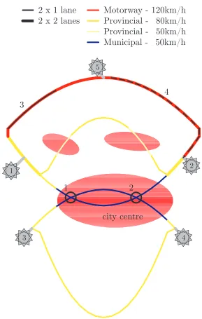
3.1 Layout of Test Network I . . . 38
3.2 Layout of Test Network II . . . 41
4.1 Radial Basis Function Network . . . 51
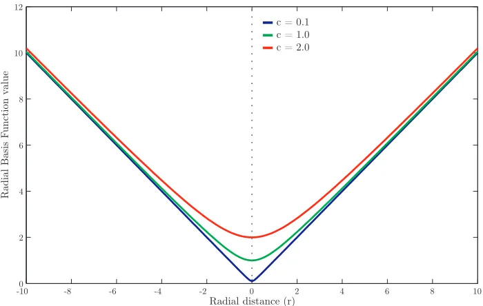
4.2 Multiquadratic Radial Basis Function . . . 53
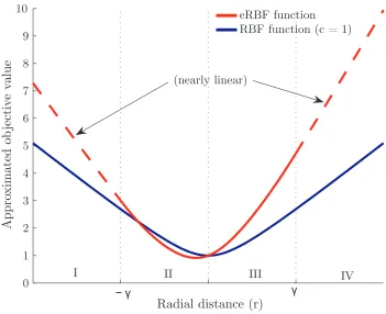
4.3 extended Radial Basis Function . . . 54
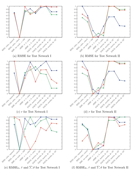
4.4 Overview of Best Scoring Approximation Variants . . . 77
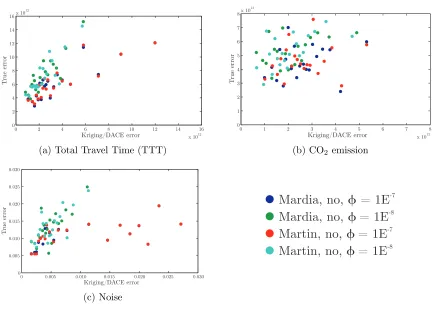
4.5 True vs Kriging/DACE Errors . . . 78
6.1 Example of the S- and D-Metric performance measures . . . 96
6.2 Example of the ∆ and ∆′ performance measure . . . 100
6.3 Performance Measures for Test Network I . . . 106
6.4 Pareto front for Test Network I . . . 107
6.5 Performance Measures for Test Network II . . . 109
6.6 Pareto front for Test Network II . . . 110
6.7 Performance Measures for 100 Final Parents . . . 112
6.8 Convergence of exactly evaluated solutions . . . 113
6.9 Example of expected behaviour of Probability of Improvement in combination with Kriging/DACE . . . 115
7.1 Overview of Almelo Area . . . 120
7.2 Road Network of Almelo . . . 121
7.3 DTM measures on the Almelo network . . . 122
7.4 Performance Measures for the Almelo Network . . . 124
7.5 Pareto Front for the Almelo Network . . . 125
7.6 Example Boxplot of the Effects of DTM measures . . . 127
7.7 Projections of Pareto front with and without rare settings . . . 130
C.1 Pareto front for a biobjective problem with one known solution . . 156
C.2 Strictly dominating and Augmenting solutions . . . 157
C.3 Example for determining PoIaug . . . 158
C.4 Probability cube for a problem with three objectives . . . 159
List of Tables
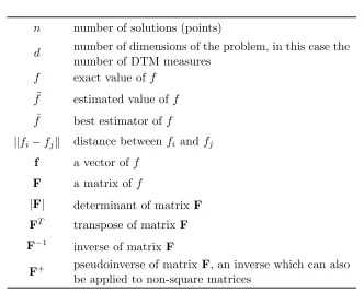
1.1 Notation in Objective Functions . . . 11
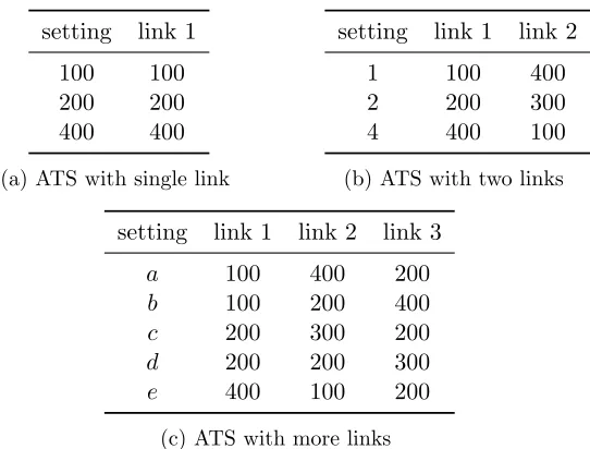
2.1 Examples of Different ATS Setting Scales . . . 30
2.2 Overview of Variables for each of the DTM Measures . . . 33
3.1 Settings of DTM Measures for Test Network I . . . 38
3.2 Settings of DTM Measures for Test Network II . . . 42
4.1 Notation in Approximation Methods . . . 47
4.2 extended Radial Basis Function Values for φ . . . 54
4.3 Possible Outcomes Domination Quality Measure . . . 66
4.4 Variable Values for Response Surface Method . . . 68
4.5 Variable Values for Radial Basis Functions . . . 68
4.6 Variable Values for Kriging/DACE . . . 68
4.7 Best Methods for Approximating Objective Values (RMSEΣ) . . . 75
4.8 Best Methods for Approximating Objective Values (ˆr). . . 75
4.9 Best Methods for Prediction Decisions (ϑ) . . . 76
4.10 Calculation times for Approximation Method Variants . . . 76
4.11 Values of aandR2 for Kriging/DACE methods . . . 79
4.12 Values of a,b and R2 for Kriging/DACE methods . . . . 79
5.1 Categorisation of MAEA approaches . . . 85
6.1 Overview of AMAN approaches . . . 92
A.1 DTM control settings for Test Network I . . . 151
B.1 DTM control settings for Test Network II . . . 153
D.1 DTM control settings for Almelo . . . 162
List of Algorithms
1.1 NSGA-II . . . 13
1.2 Non-dominated Sorting Algorithm . . . 14
1.3 Crowding Distance Algorithm . . . 14
5.1 Inexact Pre Evaluation (IPE) . . . 86
5.2 Probability of Improvement (PoI) . . . 87
List of Abbreviations
AE Algorithmic Effort
AMAN Approximation Model Assisted NSGA-II
ATS Automated Traffic Control Signal (traffic light)
DTA Dynamic Traffic Assignment
DTM Dynamic Traffic Management
EA Evolutionary Algorithm
EI Expected Improvement
eRBF extended Radial Basis Function
FAS Fraction of Acception Solutions
GA Genetic Algorithm
GTC Generalised Travel Cost
IPE Inexact Pre Evaluation
MAE Mean Average Error
MAEA Metamodel Assisted Evolutionary Algorithm
MLE Maximum Likelihood Estimation
MOEA Multiobjective Evolutionary Algorithm
MOGA Multiobjective Genetic Algorithm
NDP Network Design Problem
PoI Probability of Improvement
POS Pareto optimal set
RBF Radial Basis Function
RMSE Root Mean Squared Error
RNI Rate of Non-dominated Individuals
RSM Response Surface Method
SA Simulated Annealing
SO System Optimum
STA Static Traffic Assignment
SUE Stochastic User Equilibrium
TS TABU Search
TT Travel Time
TTT Total Travel Time
VLS Variable Lane Sign
VMS Variable Message Sign
Chapter
1
Introduction
Traffic is only one of the side effects of growth.
Roy Barnes (1948 – )
The quote by Roy Barnes can, in a way, be considered the starting point of this research. Due to the continuous economic growth the demand for traffic has been increasing over the past decades. Not just in the United States of America, to which Roy Barnes probably was referring, but also in Europe and especially in a densely populated area such as the Netherlands.
In the past the solution to the traffic demand problem was found in construct-ing new infrastructure, but this is no longer a viable option as we will infer in section 1.1. The solution that is currently in favour, the use of Dynamic Traffic Management, brings along some other challenges. One of the problems is that there are many different ways in which Dynamic Traffic Management can be applied and we therefore have to define which solutions are considered to be optimal.
In order to be able to determine the effect of different solutions of Dynamic Traffic Management, we first have to define a framework which can be used to model Dynamic Traffic Management measures. In section 1.2 we will therefore explain why the Network Design Problem is a suitable framework for modelling DTM measures. Unfortunately we will also show that it is virtually impossible to find optimal solutions, which is why we have to resolve to algorithms to find good solutions. Consequently we introduce three different algorithms in section 1.3 and will elaborate more on one specific family of algorithms, which are the Genetic Algorithms.
Up to this point we have been diverging the subjects of our research to an extend where we are unable to complete the research within a reasonable period of time. In section 1.4 we therefore determine the scope of this research, by limiting the number of objectives that we are trying to attain. Furthermore
we will select a single modelling framework (from section 1.2) and a single algorithm (from section 1.3) with which we will continue our research.
Something that is probably just as important, is defining the main goal of this research. We therefore first have to determine which problems we can identify and decide how we would like to solve these problems. In section 1.5 we will accordingly briefly discuss two problems that we have identified and select one specific problem, after which the (main) goal of this research can be formulated.
It is at this point that we can, using the results from section 1.4 and 1.5, determine which subjects are relevant for the remainder of the research. In section 1.6 we therefore start by creating a research model, which provides an overview of the different subjects we need to study in detail. In section 1.7 we continue by defining the questions that have to be answered, before we have enough knowledge about the subjects from the research model. Finally in section 1.8 we will explain how we will obtain the information to answer the research questions.
Finally, having defined the main goal of our research and the strategy which we will follow to attain this goal, we will provide an outline of this thesis (section 1.9). In this outline we will explain where you are able to find the answers to the different research questions, and as such where the different subjects are discussed.
Let us now start by introducing the Dutch problem and Dynamic Traffic Management.
1.1
The Dutch Road Network & Dynamic Traffic
Management Measures
In the past decade(s) the Dutch road network has become increasingly busy and traffic-jams are a day-to-day practice for most commuters. In the past these problems might have been tackled by expanding the existing road net-work by constructing new roads or expanding existing ones. European legisla-tion, however, restricts the construction of new roads, by enforcing new rules concerning air and noise pollution. Furthermore there are problems related to the increasing costs of expanding road networks, the time that is required before work can actually start, and a lack of space. Dutch authorities have therefore resolved to using the existing road network more efficiently rather than expanding the current road network.
1.1. The Dutch Road Network & DTM Measures 3
the first is the DTM measure that can be adjusted quite swiftly (but not instantaneous). The most widely known example of such a DTM measure is the Automated Traffic Control Signal (ATS). It is quite easy to change the settings of an ATS (which influences the capacity of the crossing in a certain direction) but this is rarely done in real-time.1 The second type of DTM measure is able to make changes instantly, thus enabling the authorities to react upon the current state of the network (real-time adjustment of the DTM measure), or can be made in a quite short period of time. One of the most commonly used examples of this type of DTM measures is the so-called Variable Message Sign (VMS). These signs can be used to limit or increase the number of lanes (‘crossing off’ lanes, allowing shoulder lanes to be used) which directly influences the capacity of a specific road section, impose variable speed limits and provide travel time, traffic-jam and other information to road users which they can use to alter their route choice. ATS and VMS are therefore amongst the most powerful tools in directing traffic.
In order to determine the resulting traffic conditions of a solution usually a Dynamic Traffic Assignment (DTA) is used, which propagates traffic through a network, simulating the behaviour of traffic over a period of time. These DTA models are well suited to predict the results of different DTM measures, as long as they influence the characteristics of the network (i.e. they should influence speed or capacity of a specific road section). Although DTA models can also be used to predict the effects of non-network changing DTM measures, such as advanced traffic information, this does require a good behavioural model, which is often not available.2 Using the results of these DTAs (flows and speeds on road sections) the effects on travel time, air and noise pollution and road safety (or other objectives) can be estimated.
As mentioned earlier it is possible to use DTM to influence the behaviour of road users in real-time. However it is also possible to use DTM to provide the road users (in fact all those involved) with the ‘best’ road network possible. In that case for each time of the day a decision should be made concerning the settings of the DTM measures, a so called ‘strategic’ policy. Deciding which DTM measures should be implemented and when (which is what makes them dynamic) is one of the most difficult decisions in traffic engineering. Good examples of such ‘strategic’ policies are the speed limits of 100 and 80 km/h on motorways around major cities and the use of additional lanes during peek hours. However the application of these measures seems quite arbitrary. The measures are implemented to attain a single objective, for instance reduction
1The ATS under consideration here is the ATS with a fixed cycle, the more and more
common ATS with detection loops do of course adapt their cycle in real-time.
2The behavioural model is here defined as a model that predicts which fraction of people
objective function 1
ob
jectiv
e function 2
A,D
B
C
(a) Example of Dominance
objective function 1
ob
jectiv
e function 2
(b) Example of Pareto front
Figure 1.1: Dominance and Pareto fronts
of noise, reduction of air pollution, reduction of travel times or (although less frequently used) reduction of the number of casualties and fatalities. Therefore the question arises whether the DTM measures, that are currently applied, might have a deteriorating effect on other objectives. Therefore research has started that tries to find a set of possible settings for DTM measures (for a certain problem area), which are not dominated by other solutions.
In order to understand which solutions are called non-dominated we first have to study the concept of dominance. We will explain dominance us-ing Figure 1.1a. Let i be the index of the objective functions, a and b are two solutions and fi(a) is the objective value for solution a on objective i. Furthermore assume a minimisation problem. First there is the concept of
weak dominance, we say thata weakly dominatesb (denoted byab) when
∀i fi(a)≤fi(b). In Figure 1.1a this means thatB,C and Dall weakly dom-inateA. Next there is dominance,ais said to dominateb (denoted bya≻b) when∀i fi(a)≤fi(b)∧ ∃i:fi(a)< fi(b). In Figure 1.1a we can therefore say that bothB andC dominateA. Finally there isstrong dominance,astrongly dominates b (denoted by a ≻≻ b) when ∀i fi(a) < fi(b). In Figure 1.1a B strongly dominatesA.
Back to our original problem we can now state that we are looking for solutions
1.2. Network Design Problems 5
In the next section we will explain why (and how) our problem can be de-scribed as a Network Design Problem. Furthermore we will provide a brief overview of traffic and transport related Network Design Problems in literat-ure.
1.2
Network Design Problems
A formal (mathematical) Network Design Problem (NDP) usually starts with a given (un)directed graph G= (V, E) a cost ce for each e ∈E (or for each arc in the directed case), and we like to find a minimum cost subset E′ of the edges E that meets certain design criteria. The problem described above (selecting DTM measures in order to attain certain objectives) can easily be translated to a directed NDP. The graphGconsists of a set of links (E), which are connected to each other at a vertex (V). In this case each DTM measure adds one or more arcs e to an edge E, which gives the possibility to select a subset E′ that optimises the objectives.
Literature suggests two ways of modelling the design variables, either dis-crete using the Disdis-crete NDP (DNDP) or continuous using the Continuous NDP (CNDP). The DNDP models are used when the construction of new links (or even complete networks) is considered (see: Poorzahedy & Turnquist, 1982; Drezner & Wesolowsky, 2003; Gao, Wu & Sun, 2005), whilst the CNDP models are used when only the expansion of existing links (e.g. a change in capacity or maximum speed) is considered (see: Meng, Yang & Bell, 2001; Chiou, 2005; Zhang & Lu, 2007; Mathew & Sharma, 2009; Xu, Wei & Wang, 2009; Chen, Kim, Lee & Kim, 2010). However the expansion of an existing link is often a discrete problem, one either adds another lane or one does not. In that sense the use of a CNDP can be considered a relaxed version of the problem, which is why DNDP models can also be used to model expan-sion problems (see: LeBlanc & Abdulaal, 1978; Boyce & Janson, 1980). It is therefore that we decided to model our problem as a DNDP.
Our problem should be described as a bilevel optimisation problem (bilevel NDP). This is due to the fact that there are two decision makers involved (road users and authorities) which have different objectives (Chen et al., 2010). Due to the difference in objectives, a kind of game arises in which the authorities set their decision variables in such a way that their objectives are optimised (upper level optimisation), to which the road users respond by changing their route choice (lower level optimisation). To this change in route choice the authorities respond by adjusting their decision variables, and these reactions circle until convergence has been reached (Figure 1.2).
Road Authorities set DTM in order to optimise the objectives
Road users change routes to optimise travel time
DTM link flows,
objective values
Figure 1.2: Bilevel Network Design Problem
travel time (TT) or (generalised) travel cost (GTC). This minimisation is attained when the so-called (Stochastic) User Equilibrium (SUE or UE, also known as user optimum) is reached, a point in which no road user can reduce his (or hers) objective by changing to another route. (see: Poorzahedy & Turnquist, 1982; Chiou, 2005; Gao et al., 2005; Poorzahedy & Rouhani, 2007; Zhang & Lu, 2007; Xu et al., 2009; Chen et al., 2010). This is in accordance with (and also known as) the first principle of Wardrop, which states ‘the journey times in all routes actually used are equal and less than those which would be experienced by a single vehicle on any unused route’ (Wardrop, 1952). For the upper level the objective is usually to minimise total travel time (Gao et al., 2005; Poorzahedy & Rouhani, 2007; Zhang & Lu, 2007) or travel cost (Poorzahedy & Turnquist, 1982) over the entire network, also known as the System Optimum (SO). At this SO the second principle of Wardrop ‘at equilibrium the average journey time is minimum’ (Wardrop, 1952) applies. When no budget constraints are used in the bilevel NDP, the construction costs can be incorporated in the upper level objective function (Chiou, 2005; Xu et al., 2009). There are only a few papers which use multiple objective functions in the upper level, Chen et al. (2010) use travel time (SO) and construction costs as two separate objective functions, Cantarella and Vitetta (2006) use in-vehicle travel time, access and egress time as a result of parking and CO emissions as their upper level objective functions whilst Friesz et al. (1993) focus on minimising the transport costs, construction costs, vehicle miles travelled and house removal. Sharma, Ukkusuri and Mathew (2009) who provide an overview of multiobjective optimisation for transport NDP are only able to list six papers. This shows that there is very little experience with using externalities as objective functions in bilevel NDP.
1.3. Genetic Algorithms 7
is not possible (at least in reality) because the number of possible solutions usually is very large.3 Determining a single lower level optimisation (using DTA to determine the SUE) in a realistic network easily takes an hour, which means that a full enumeration would take forever.4
In the next section we will introduce Genetic Algorithms and explain why they can be used to reduce the computational effort of searching for the Pareto optimal set.
1.3
Genetic Algorithms
Because the bilevel NDP is a NP-complete problem, a more intelligent ap-proach has to be used in order to find (or at least approximate) the Pareto optimal set (POS). For these kind of problems a lot of algorithms (also known as metaheuristics) have been developed. These metaheuristics, which are de-veloped since the 90s of the previous century, have proven themselves to be flexible and are capable of finding good solutions, even when non-standard objectives and binary or integer variables are involved (D. F. Jones, Mirrazavi & Tamiz, 2002). Unfortunately most of these heuristics focus on single ob-jective problems. If we limit ourselves to algorithms that can be modified to work with multiobjective problems, Genetic Algorithms (GAs, also known as Evolutionary Algorithms; EAs), Simulated Annealing (SA) and TABU Search (TS) are the most commonly used algorithms (see for instance the book by Pham and Karaboga (2000) for an overview of these algorithms).
There is very little literature available about which algorithm will per-form best when being confronted with a multiobjective NDP. In fact even when only considering single objective problems, literature still is uncertain which algorithm performs better. Youssef, Sait and Adiche (2001) applied the three algorithms to a floor planning problem and concluded that TS was best (both in results and computational effort) but GA was a close second (though required a lot of computational effort). Arostegui, Kadipasaoglu and Khu-mawala (2006) applied the three algorithms to the facility location problem and concluded that TS was to be preferred, since it was a more simple approach and was less dependent on the selection of parameters. Strangely Kannan, Slo-chanal and Padhy (2005) concluded more or less the opposite when applying several algorithms to an investment planning problem, they found that TS is amongst the worst solutions. Drezner and Wesolowsky (2003) found that TS en GA were alternating the best solution, but decided that GA was in the end the better approach. Braun et al. (2001) compared eleven heuristics and concluded that GA was the best (although a relatively simple approach was a
3Consider a problem with two ATSs, each with ten possible settings and six time periods,
the number of possible solutions is 1026
= 1012or one trillion solutions.
4In fact if each DTA took only 1 second, the full enumeration of the previous example
good second) and Alabas, Altiparmak and Dengiz (2002) chose TS to be the best algorithm, but this was solely based on the fact that TS only needed to evaluate a small part of the solution space. Taking into account that in the multiobjective NDP searching a large part of the solution space could even be considered an asset (something that is also recognized by Lau, Ho, Cheng, Ning & Lee, 2007) it is difficult to determine which algorithm is better. Note that none of these papers focussed on multiobjective problems, something that was taken into account in Possel (2009). He applied GA and SA to a problem similar to the one under consideration now (a multiobjective NDP, with ex-ternalities as upper level objective functions) and concluded that GA is most likely the better algorithm. Based on these studies it seems that GA could be considered a practical algorithm, something that is also reflected in the use of this algorithm in studies towards NDP (see: Gen, Cheng & Oren, 2001; Chakroborty, 2003; Drezner & Wesolowsky, 2003; Gen, Kumar & Kim, 2005; Cantarella & Vitetta, 2006; Cantarella, Pavone & Vitetta, 2006; Poorzahedy & Rouhani, 2007; Zhang & Lu, 2007; Schm¨ocker, Ahuja & Bell, 2008; Mathew & Sharma, 2009; Sharma et al., 2009; Xu et al., 2009; Chen et al., 2010).
Genetic algorithms are the invention of John Holland (Holland, 1975) and are based on the biological process of ‘natural selection’. The main idea is that each solution (‘chromosome’) can be described by a series of bits (‘genes’), i.e. each solution is described by the state of each explanatory variable. These biological terms are used because the algorithm mimics the process of com-bining two strings of DNA into one or two others. The algorithm moves from one population of ‘chromosomes’ to another by crossover (combining two ‘parents’ into one or two ‘children’, the ‘offspring’), mutation (randomly changing the ‘genes’ of the ‘chromosome’) and inversion (inverting the ‘genes’ of a ‘chromosome’). By selecting only the best solutions found in the total set of ‘parents’ and ‘offspring’ the algorithm ensures that good solutions can be found, whilst preventing itself from finding only local optima. This algorithm has proven itself in the past decades, since it has been applied to numerous problems in the fields of optimisation, economics, immune systems, social sys-tems etc. (Mitchell, 1996). Genetic algorithms, as discussed in the previous paragraph, are designed to find a single optimal solution. However, due to the nature of the algorithm, using a population of solutions, the algorithm can easily be modified in order to cope with multiobjective problems.5 If one selects the population to be large enough, this population will (eventually) describe the Pareto optimal set. This is why at the end of the previous cen-tury (and at the beginning of the current one) a lot of research has been done in developing Multi Objective Genetic Algorithms (MOGAs), the best known examples are Non-dominated Sorting Genetic Algorithm (NSGA; Srinivas &
5Genetic Algorithms only require that one is able to determine whether a solution is
1.4. Research Scope 9
Deb, 1994), Strength Pareto Evolutionary Algorithm (SPEA; Zitzler & Thiele, 1999), Pareto Envelope-based Selection Algorithm (PESA; Corne, Knowles & Oates, 2000) and Pareto Archived Evolution Strategy (PAES; J. D. Knowles & Corne, 2000a). In a fierce competition amongst followers of the different algorithms, each algorithm was proven to be better than others in certain test problems. Therefore additions and alterations were made to each of the al-gorithms, which resulted in M-PAES (J. D. Knowles & Corne, 2000b), PESA-II (Corne, Jerram, Knowles & Oates, 2001), SPEA2 (Zitzler, 2001), NSGA-PESA-II (Deb, Pratap, Agarwal & Meyarivan, 2002) and finally SPEA2+ (M. Kim, Hiroyasu, Miki & Watanabe, 2004).
It is difficult to determine which algorithm is better, since each one out-performs others in specific test problems. It is also not clear if any of these ap-proaches should be preferred when considering traffic related problems. Most papers (see the list mentioned earlier) do use GAs, but do not use a specific predefined GA. In fact only three studies that use a specific predefined GA have been found. Sumalee, Shepherd and May (2009) use NSGA-II in their optimisation of road charges and both Possel (2009) and Sharma et al. (2009) studied a NDP with budget constraints. Although not using predefined GAs might have advantages (one can optimise the GA for a specific case) it fails to take advantage of research that has already been done in this field.
1.4
Research Scope
In the previous three sections we described how DTM measures could be used to optimise traffic flows, how such a process could be modelled and which algorithms can be used to find (or better: approximate) the Pareto optimal set. In this section we will be more specific and decide which specific solutions and approaches we will use throughout this research.
This research will focus solely on DTM measures that directly influence net-work properties. This means that a DTM measure either influences the speed (in fact speed limit) or the capacity of certain links in the network. This is done because these DTM measures can fairly easy be modelled in existing transportation models, whereas modelling DTM measures that influence be-haviour (e.g. traffic jam information) require extensive bebe-havioural models. This leaves only three specific DTM measures that will be considered, which are listed below.
Automated Traffic Control System (ATS) In reality an ATS would
Variable Speed Sign (VSS) These signs alter the maximum speed on cer-tain links;
Variable Message Sign (VMS) Although in reality these signs can be used
for a multitude of things, in this research we will limit its possibilities to adding or removing additional lanes. These lanes can be either a rush-hour lane, which usually is the hard shoulder of a motorway, or a reversible lane. We will refer to this specific use of VMS as Variable Lane Sign (VLS).
It is important to note that these measures will be applied dynamically, i.e. they are allowed to change over time. This means that authorities can create different optimal settings, e.g. for night, morning rush hour, daytime and evening rush hour periods. Of course it is also possible to use different settings within a single rush hour period. This does however also affect the method that is used to determine the user equilibrium that is attained, something that will be addressed later on.
We also limit the number of objectives that we like to attain by using DTM. The main reason for limiting the number of objectives is that adding more objectives only increases computational effort, without significantly contribut-ing to this research. Furthermore it is important that the selected objectives do not have a positive proportionality constant, otherwise minimising one objective would automatically minimise the other. It should be possible to determine the objective value using the information from the network model and the DTA, this means that objective values should be determined using nothing more then maximum speed, capacity, road type, speed and intensity. Therefore three objectives have been selected, each representing another part of the effects that are caused by traffic. In the equations used to describe the objective values, the notation from Table 1.1 is used.
The first objective is the minimisation of congestion, which is measured using the Total Travel Time (TTT; hours). This is probably one of the most used objectives because it tries to attain an optimal solution from a transportation system point of view (SO). Note that this is not the same as the stochastic user equilibrium (SUE) solution that is used in the lower level optimisation. The value of this objective function can easily be determined using:
z1 =T T T = X
k
X
t
X
m
fm k (t)lk
vm k (t)
(1.1)
The second objective is to minimise pollution, which is measured using CO2
1.4. Research Scope 11
lk length of link k
δkd indicator for road type, 1 if road kis of typed, 0 oth-erwise
δkw indicator for urbanisation level, 1 if roadw, 0 otherwise k is of level
ηw correction factor for urbanisation level w(dB(A))
αm, βm noise parameters for mode m
Vmref reference speed for mode m (km/h)
fm
k (t) vehicle inflow on link kduring time periodt (veh)
vmk(t) average speed on linkkduring time periodtfor mode
m (km/h)
ECO2
md (·)
CO2emissions of modemdepending on average speed
(grams / veh ·km)
Lm(·) average sound power level for modeaverage speed (dB(A)) m, depending on
¯
Lw weighted average sound power level on the networkwith urbanisation level w(dB(A))
Table 1.1: Notation in Objective Functions
model database and the following equation:
z2 =CO2 = X k X t X m X d
fkm(t)δkdEmdCO2(vkm(t))lk (1.2)
The third and last objective is to minimise noise, which is measured using the weighted average sound power level at the source (dB(A)). This can be determined using the Dutch standard method (Ministry of Housing, Spatial Planning and the Environment, 2002):
z3 =noise= 10·log P
k
P
wδkwlk10
¯
Lw−ηw
10
P
k
P
wδkwlk
!
with ¯Lw = 10·log
P
k
P
wδkwlkPm10
Lm(·) 10
P
k
P
wδkwlk
!
withLm(·) =αm+βmlog
vkm(t)
vref
m
+ 10·log
qkm(t)
vkm(t)
(1.3)
Assignment model (STA) to optimise the lower level problem, we will use a Dynamic Traffic Assignment model. The main reason for using a DTA instead of an STA is that we would like to be able to change the settings of the DTM measures during the day (in order to allow specific schedules for e.g. morning and evening rush hours or even changing schedules within a rush hour). Al-though this could be modelled using STA in quite small networks (the point at which one reaches a DTM measure is more or less the same as the departure time) this is virtually impossible in larger (real sized) networks. In that case only DTAs are able to give (fairly) good predictions of the changing traffic flows over the network.
In this research we therefore use the software program OmniTRANS (ver-sion 5.1) which uses the Macroscopic DTA called Streamline. This model is based on an adaptation of the fluid transmission model by Messmer and Papageorgiou (1990), which was based on the model by Payne (1971), and uses the single-regime speed-flow-density relationships of Van Aerde (1995).
Because the upper level of the bilevel NDP is a NP-complete problem, a metaheuristic is used to approximate the optimal solution. From literature (see the discussion in section 1.3 about Genetic Algorithms) it is clear that genetic algorithms prove to be a good approach when struggling with complex (hard) problems. Especially NSGA-II (Deb et al., 2002) appears to be robust and capable of creating good solutions when applied to traffic related bilevel NDPs (Possel, 2009; Sumalee et al., 2009). Therefore the NSGA-II algorithm is chosen as the algorithm that will be used in this study.
The approach that is used to solve the bilevel NDP combines the knowledge about bilevel programming, Dynamic Traffic Assignments, Genetic Algorithms and externalities. Let us start by explaining the NSGA-II algorithm, which is shown in Algorithm 1.1 in more detail.
The algorithm starts withN exactly evaluated parent solutions (P0), which
can be generated using Random Sampling (RS), Stratified Sampling (SS), Latin Hypercube Sampling (LHS) or any other sampling approach (McKay, Beckman & Conover, 1979). Based on the objective values the fitness of each solution can be calculated using the non-dominated sorting and crowding dis-tance algorithm. The non-dominated sorting algorithm which is shown in Al-gorithm 1.2 determines for all solutions the rank of the Pareto front in which they are located. The crowding distance algorithm, shown in Algorithm 1.3, determines per front which solutions are farthest apart from all the other solu-tions in that front. Solusolu-tions that are farther apart are considered to be more valuable and thus get a higher fitness value. TheN best performing solutions are stored as the parents for the next generation (Pg+1) and the remainder
are stored in a databaseDthat is used to prevent exactly evaluating the same solutions twice. If we have reached the maximum number of generations G
1.4. Research Scope 13
Algorithm 1.1 NSGA-II
1. Initialisation
Start withN exactly evaluated parent solutionsP0
Define a set of offspringQ0 =∅
Define a database for previously evaluated solutionsD=∅
Furthermore define the maximum number of generations G and set
g= 0
2. Fitness Assignment
CombineRg=Pg∪Qg
Determine fitness value by dominance and crowding distance
3. Selection
SelectN best solutions (based on fitness) from Rg and store asPg+1
Store remaining solutions in database,D=D∪(Rg\Pg+1)
4. Termination
Ifg≥Gterminate the algorithm, otherwise continue with step 5
5. Mating selection
Perform binary tournament selection with replacement and repair on
Pg+1 to determine mating poolP′g+1
6. Variation
Apply recombination and mutation to mating pool P′g+1 to create
offspringQg+1
7. Function Evaluation
Determine objective values for all solutions inQg+1
Setg=g+ 1 and continue with step 2
which will mate in order to create N new children (Qg+1). We then exactly
evaluate the solutions in the offspring set (Qg+1), updateg and continue with
step 2, i.e. we determine the fitness of the solutions in the combined set Rg. When we state that we ‘exactly evaluate the solutions’ we follow the pro-cedure as shown in Figure 1.3. The NSGA-II algorithm provides OmniTRANS with the settings for the different DTM measures6 for all time periods. For
each solution OmniTRANS first determines the resulting links flows and link speeds, after which these results (i.e. link flows and link speeds) are converted to objective values using the objective functions (equations 1.1–1.3), which is actually done by MatlabR for computational convenience. The final objective
Algorithm 1.2 Non-dominated Sorting Algorithm (Deb et al., 2002)
for allp∈P do
Sp =∅
np = 0
for all q∈P do
if p≺q then ifpdominates q
Sp =Sp∪ {q} add p to the set of solutions dominated byq
else if q ≺p then
np =np+ 1 increment the domination counter of p
if np = 0 then pbelongs to the first front
prank = 1
F1 =F1∪ {p}
i= 1 initialize the front counter
while Fi 6=∅ do
U =∅ used to store the members of the next front
for all p∈ Fi do
for allq∈Sp do
nq=nq−1
if nq = 0then q belongs to the next front
qrank =i+ 1
U =U ∪ {q} i=i+ 1
Fi =U
Algorithm 1.3 Crowding Distance Algorithm (Deb et al., 2002)
l=|F| lis the number of solutions in F
for alli= 1. . . ldo
F[i]distance = 0 initialise distance
for allobjectiveso do
sort F on objectiveo
F[1]distance=F[l]distance =∞ ensure that boundary points are always selected
for i= 2. . . l−1 do for all other points
1.5. Research Goal 15
NSGA-II
OmniTRANS
use DTA (StreamLine) to determine the Dynamic SUE and corresponding link flows and link speeds
use objective functions to determine objective values
settings for DTM measures
objective values
Matlab®
link flows and link speeds
Figure 1.3: Procedure for Exactly Evaluating Solutions
values are returned to NSGA-II to be used for the fitness assignment.
The problem solving method described above gives indeed good solutions to the problem of minimising traffic externalities using DTM measures (Wismans, Van Berkum & Bliemer, 2009, 2010). And although a MOGA is already a much more intelligent approach than complete enumeration, it still needs to evaluate a lot of solutions (DTAs and objective evaluations) which makes that it easily takes months to solve a real-life problem. Secondly, there is very little protection from evaluating solutions that are prospectless, which means that computational time is spend in vain.
1.5
Research Goal
should be used more efficiently by only evaluating favourable solutions. A possible way to attain this situation is by developing a method that is able to quickly estimate the objective value of a possible solution (i.e. without evaluating the solution using a DTA) and use the result of this evaluation within the optimisation process (e.g. to determine whether this solution should be evaluated by a DTA). When focussing on this specific problem, we see that there are already a number of solutions available (these solutions are needed as ‘parents’ for the GA) which could be used in the problem solving method. For single objective optimisation problems a well-known method is the trust region optimisation (see e.g. Conn, Gould & Tointe, 2000). This method uses an approximation method (also known as metamodel or surrogate model) to evaluate solutions. There are many different approaches that can be used to approximate the objective values. Another well-known method (often used in social sciences) is regression analysis, which tries to fit a model to a set of known solutions. Besides the standard linear regression functions a variety of non-linear and multivariate functions exist, all serving a specific type of parameters and goal functions. These functions approximate the results of the DTA and could be used to determine whether a specific solution is interesting enough to be evaluated by the DTA.
It seems that a well chosen approximation model, in combination with the right explanatory parameters could be used to give a first estimate of the results of a specific set of DTM measures. To the best of our knowledge such an approach has not yet been developed or applied to a NDP, and the main goal of this research is therefore defined as:
accelerating the search for the Pareto optimal set found by mul-tiobjective genetic algorithms for mulmul-tiobjective network design problems, in which externalities are the objectives and DTM meas-ures the decision variables, using function approximations.
Besides predicting whether a solution is interesting enough to be evaluated by a DTA, approximations can be used in a number of ways. It would for instance be possible to use the approximations to determine in which area more data is required to improve the approximations, or the approximations can be used to determine the results in areas in which a lot of information is available. This means that several ways in which the Pareto optimal set can be improved will be investigated, however which ways are viable is dependent on the accuracy of the approximation function.
1.6
Research Model
1.7. Research Questions 17
Improving the Pareto optimal set
Pareto Front assessment criteria
Possible improvement methods
Approximation methods Acceleration possibilities
Metamodel assisted EA Approximation literature Performance measures
Figure 1.4: Research Model
be drawn. This framework can then be used to define the research questions and research methodology. We therefore developed a compact research model, which is shown in Figure 1.4.
As mentioned above, the main goal is to improve the Pareto optimal set. Improving implies that there is a clear view on what is a better solution (the same solution in less time, a better solution in the same time, a solution of which a higher percentage is indeed part of the Pareto optimal set, etc.) and therefore the subject of Pareto front assessment criteria should be investigated. These criteria can than be used to determine whether a solution (i.e. Pareto front) is better. Based on these criteria a set ofpossible improvement methods
can be evaluated.
This set of possible improvement methods should be derived from the combination of approximation methods andacceleration possibilities. The ap-proximation methods will be derived from literature and will be selected based on their performance on test cases. The acceleration possibilities will also be derived from literature, but we will select suitable ones based on how well they can be integrated in NSGA-II.
1.7
Research Questions
where there are opportunities to incorporate ‘intelligence’ into this genetic algorithm. The third research question focuses on how the results of the two previous questions can be combined into a single improvement method. And finally the fourth and last research question applies the developed methods from question three onto a realistic problem network. For each research ques-tion a set of sub quesques-tions can be defined that explore the subject in greater detail. This results in the following research questions:
1. How can the objective values of the bilevel NDP be approximated?
a) What approximation methods are used for complex problems in literature?
b) What data is needed in order to ‘feed’ these methods?
c) How ‘good’ do these methods approximate the ‘true’ objective val-ues?
i. Which criteria can be used to determine ‘good’ ?
ii. How do these methods score on these criteria when applied to two different test networks?
2. In what way can the genetic algorithm be accelerated?
a) How can the genetic algorithm be accelerated according to literat-ure?
b) Where in the genetic algorithm could ‘intelligence’ be incorporated?
c) What intelligence can be incorporated in the genetic algorithm?
3. Which improvement methods do indeed improve the search for the Pareto optimal set?
a) Which approximation methods can be incorporated in the genetic algorithm?
b) Which criteria can be used to describe an improvement of a Pareto optimal set?
c) How do the improvement methods score on these criteria?
4. How do these methods cope with realistic networks?
1.8. Research Methodology 19
1.8
Research Methodology
Main goal of defining a research methodology is to determine up front which approach is to be used to answer a specific research question. Suitable ap-proaches could for instance be literature study, interviews, testing and simu-lation studies. In this thesis we decided to opt for two main approaches which are literature study and testing. The former approach is mainly used to de-termine what the current ‘state of the art’ is on a specific topic, whereas the latter is used to check whether a chosen model or approach is suitable for our problem.
In the remainder of this section we will discuss the methodology used, by answering the question ‘what do we do, and why do we do it?’
In order to answer research question 1 we decided to perform a literature study into approximation methods, where we focus on approximation methods that are commonly used in combination with optimisation problems. Furthermore we prefer approximation methods that are known to be combined with Genetic Algorithms. So why do we perform a literature study?
Probably the most important reason is that we would like to get a good idea how the different approximation techniques work. It would for instance be interesting to see which equations and/or algorithms are required to obtain the approximated objective values for, after all, applying an approximation method that is so complicated that it requires more time than exactly evalu-ating the objective values is of little use. Furthermore we need to know which information is needed as input data for the approximation techniques, since we have to be able to provide this information. Perhaps just as interesting are the different variants that might have been applied in the past, because they have often been optimised for a specific problem. Similarly it is interesting to see which (predefined) parameters are part of the approximation techniques, since they could be used to ‘fine tune’ the approximation technique.
It seems that after this literature study we should have a good and com-plete overview of the possibilities of the different approximation techniques. In order to reduce the complexity of the research, it seems requisite to reduce the number of variants (i.e. different variants or different parameter settings) of approximation techniques. It seems appropriate to combine this reduction with research question 1c which makes that we a) have to perform a liter-ature study into quality measures for approximation techniques; and b) test which of the variants of the approximation techniques appear to be the ‘best’ according to these quality measures.
to be part of the Pareto front, independent of the estimated objective value. We therefore also try to find quality measures that measure this phenomenon. Finally we will use the ‘testing’ approach to determine how good the vari-ants are able to approximate the objective values (research question 1(c)ii). However at the same time we will use this approach to determine which of the variants are ‘best’ (and will therefore be used in the remainder of this research). Of course there is the risk that a variant, which appears to per-form extremely well in one case, perper-forms extremely poor in another. We therefore decided to use two different road networks for the test, only variants that perform ‘good’ on both networks are considered as ‘best’ variants of ap-proximation techniques. Using two different networks therefore increases the chances that the chosen variants also perform ‘good’ on other networks.
For answering the second research question we follow a slightly different ap-proach, although the start is similar. We start by performing a literature study into the field of the Metamodel Approximated Evolutionary Algorithms (MAEAs). The goal of this literature study is to provide an overview of dif-ferent MAEA approaches that have been used in the past, and we thereby do not limit ourselves to our field of interest (i.e. we do not limit ourselves to traffic and transport related research).
It is likely that we have to reduce the number of MAEA approaches that we are going to consider in the remainder of the research. Theoretically we could use the testing approach again, however, it is likely that this would take to much time since it would require us to combine different variants of approx-imation techniques with all of the MAEA approaches. Furthermore it is likely that not all MAEA approaches can be combined with the NSGA-II algorithm or the approximation techniques that we decided to use. We therefore limit the number of MAEA approaches using more qualitative criteria such as: a) is the approach intuitive; b) can the MAEA approach be used in combination with the chosen approximation techniques; and c) what is the computational effort of the MAEA approach. Especially the latter criterion can be considered relevant, since approaches that require new optimisation and approximation models would probably require to much effort (i.e. evaluating solutions exactly might be less expensive).
At this point we have arrived at research question 3 which we will answer mainly by testing. However we start by combining the results from the pre-vious two research questions into Approximation Method Assisted NSGA-II algorithms (AMANs). We will also check whether the proposed AMANs are indeed viable, i.e. we check whether the data that is provided by the approx-imation methods is sufficient for the MAEA approaches.
1.9. Outline 21
be used to compare the different AMANs with the original NSGA-II algorithm. Since it is likely that there are many different performance measures present in literature, we decide to choose the criteria in such a way that they measure the quality of the Pareto optimal set on different aspects.
We will test the results of the different AMANs and the original NSGA-II algorithm on two different road networks, for reasons we already explained. Main goal of the testing is to determine whether the results of the AMANs are comparable to the results of the original (much more computational expensive) NSGA-II algorithm. At the end we will choose one ‘best’ AMAN based on critical discussion of the scores on the different performance measures.
The AMAN that is chosen as ‘best’ approach cannot be regarded the single best approach, but it is the approach we will use to answer research question 4. Again we will use the testing approach to answer this research question, since we want to compare the solutions that are found by the original NSGA-II al-gorithm and the selected AMAN alal-gorithm. In order to compare the solutions found by the two algorithms, we do again use the performance measures that are defined in research question 3b.
Having answered all our research questions we are able to draw conclusions, and determine whether we have achieved our research goal. Based on the results from research questions 3 and 4 we are able to determine whether the AMANs are indeed capable of producing Pareto optimal sets that are comparable to the sets that are found by the original NSGA-II algorithm. Furthermore we can determine what the possible reduction in computational effort (calculation time) is. It is this reduction in calculation time which, in combination with a comparable Pareto optimal set, can be considered the improvement of the search.
1.9
Outline
In the previous section we have explained in detail which literature studies and tests we are going to perform to answer our research questions and obtain our research goal. In this section we will provide an outline of the remainder of this thesis and explain which research questions are answered where in this document. Figure 1.5 provides an overview of this outline.
1. Introduction
7. Testcase Almelo 6. Accelerating NSGA-II
5. Metamodel Assisted Evolutionary Algorithms 4. Approximation Techniques
3. T
est Net
w
orks
8. Conclusions
2. Mo
delling Dynamic T
raffic Managemen
t
Figure 1.5: Outline of the Thesis
In chapter 2 (Modelling Dynamic Traffic Management) we discuss the problem of how we should model the different Dynamic Traffic Management measures in our Genetic Algorithm and approximation methods. As such, it is a some-what independent chapter that provides a more theoretical background for our research. Besides presenting how we model our DTM measures, we explain what the consequences of this specific model are and provide a brief discussion on how the problem size can be reduced. Furthermore we briefly explain how more complicated DTM measures than the ones used in this thesis can be modelled using our framework.
The test networks that are used in chapters 4 and 6 of this thesis, are introduced in chapter 3 (Test Networks). Not only do we discuss the char-acteristics of these networks, we also explain why these specific networks are used.
1.9. Outline 23
variants of the approximation techniques, we select two approaches that we consider to be the ‘best’ amongst the evaluated variants.
We continue in chapter 5 (Metamodel Assiste