IOA: Improving SVM Based Sentiment Classification Through Post Processing

IOA: Improving SVM Based Sentiment Classification Through Post

Processing

Peijia Li, Weiqun Xu, Chenglong Ma, Jia Sun, Yonghong Yan

The Key Laboratory of Speech Acoustics and Content Understanding Institute of Acoustics, Chinese Academy of Sciences

No. 21 North 4th Ring West Road, Haidian District, 100190 Beijing, China

{lipeijia,xuweiqun,machenglong,sunjia,yanyonghong}@hccl.ioa.ac.cn

Abstract

This paper describes our systems for expression-level and message-level sentiment analysis – two subtasks of SemEval-2015 Task 10 onsentiment analysis in Twitter. First we built two baseline systems for the two sub-tasks using SVM with a variety of features. Then we improved the systems through model iteration and probability-output weighting respectively. Our submissions are ranked the 3rd and 2nd among eleven teams on the 2015 test set and progress test set in subtask A and the 7th and 4th among 40 teams on the two test sets respectively in subtask B.

1 Introduction

Recently sentiment analysis has become one of the most popular research topics in the natural language processing community, mainly due to the exponen-tial growth of social media data replete with sub-jective information. The once neglected topic has spurred immense interests from both academia and industry. Many approaches have been proposed for sentiment analysis in customer reviews, blogs and microblogs (for good reviews, see (Pang and Lee, 2008; Liu, 2012; Kiritchenko et al., 2014)). These approaches can be roughly divided into two cate-gories. One is knowledge intensive or rule-based approaches, e.g., (Taboada et al., 2011; Reckman et al., 2013). Such approaches can achieve reasonably good results when tailored for a specific domain but their maintainability and cross domain portability is usually weak. The other is data intensive or machine learning-based, which learns to analyse sentiment

from data. It is currently the most predominant ap-proach, including supervised learning, deep learning etc. Sentiment analysis is often taken as a classifica-tion task. Widely used classifiers include Support Vector Machines (SVM), Maximum Entropy Mod-els (MaxEnt), and naive Bayes classifiers. Common features include word/character n-grams and senti-ment lexicons, among others. Key research issues for learning approaches include feature engineering, model selection, ensemble learning, etc.

SemEval 2015 task10 (Rosenthal et al., 2015) is a sequel to the two tasks on sentiment analysis in Twitter in the past two years (Nakov et al., 2013; Rosenthal et al., 2014). They have provided freely available, annotated corpus as a common testbed and significantly promoted sentiment analysis in tweet-like short and informal texts. The same metric, i.e., the average F1 score of positive and negative

classes, is used for measuring performances. But this year there are some changes. Besides the classi-cal expression-level (A) and message-level (B) sub-tasks, another three subtasks are added, i.e., subtask C – topic-based message polarity classification, task D – detecting trends towards a topic, and sub-task E – determining strength of association of twit-ter twit-terms with positive sentiment. The organisers make no distinction between constrained and uncon-strained systems, which means participants could utilise any other data. But it has to be described in the submission form.

We submitted systems only for the expression-level and message-expression-level subtasks. In this paper, we provide some details behind the systems.

Data TaskA TaskB

Twittter2013-train 7,639 7,972 Twittter2013-dev 929 1,372 Twittter2013-test 3,625 3,198 SMS2013-test 2,334 2,093 Twittter2014-test 2,028 1,561 LiveJournal2014-test 1,315 1,142 Sarcasm2014-test 124 86 Twitter2015-test 3,092 2,390 Progress2015-test 10,681 8,987

Table 1: Statistics of all the datasets. The last row of Progress2015-test data is composed of all the pre-vious test data sets.

2 Our System

Our systems are built with an SVM classifier us-ing various features and resources, includus-ing sen-timent lexicons and word vectors. To further im-prove the performance, we use model iteration and probability-output weighting.

2.1 Resources

The resources used in our system are as follows:

Labeled training and test data: Although the organisers make no difference between constrained and unconstrained systems, it is not easy to make additional data effective (Rosenthal et al., 2014). So we just use the provided labeled data. However, since we did not participate in the past two evalu-ations, we are unable to get the full labeled data be-cause some tweets are unavailable. But we crawled as much data as possible using the provided script. Table 1 shows the size of the labeled data and test data we get. The 2015 test data is released directly and the results are required to be submitted in one week. We take the training data and development data as our training data. The test data from the pre-vious years can be used for tuning parameters (but NOT for training).

Sentiment Lexicons and Word Embedding: As many researchers have showed, e.g., (Mohammad et al., 2013), sentiment lexicons play an important role in sentiment analysis. In our system, seven sentiment lexicons are used: the Hashtag Sentiment lexicon, the Sentiment140 lexicon (Mohammad and Turney, 2010), the MPQA lexicon (Wilson et al.,

Feature subtask A subtask B

word ngrams X X

POS X

clusters X

word vector X X

negation X X

lexicons X X

characters X

Table 2: Features extracted for each subtask.

2005), the Bing Liu lexicon (Hu and Liu, 2004), the AFINN-111 (Nielsen, 2011), the SentiWordNet (Baccianella et al., 2010) and the Hedonometer lex-icon1_{. In addition, as word embeddings have been}

utilised to produce promising results in various NLP applications, we use sentiment-specific word em-bedding (Tang et al., 2014) in our system.

LibSVM: We used the package LibSVM (Chang and Lin, 2011) to construct the classification model for both subtasks.

CMU Tweet NLP: It is an open resource (Owoputi et al., 2013) for analysing tweets and was used to extract features for tokenising, POS tagging and clustering.

2.2 Preprocessing

The main preprocessing steps are the following:

• All upper case letters are converted to lower case ones

• URLs and user names are replaced with strings ‘http://someurl’ and ‘@someuser’ respectively

• Tokenise and label the tweets with part-of-speech using Carnegie Mellon University (CMU) tool (Owoputi et al., 2013)

2.3 Features

After preprocessing, each tweet is represented as a feature vector made up of part of the following fea-tures, the features used in each subtask are shown in Table 2.

• Word N-grams: A binary value of contigu-ous n-grams of 1, 2, 3, and 4 tokens and non-contiguous n-grams (n=3, 4). Non-non-contiguous

n-grams are those intermediate grams that are replaced with a special symbol like ‘*’. For ex-ample, a 4-gram “I * * guys” is the correspond-ing non-contiguous gram of contiguous gram “I love you guys”.

• Character N-grams: Although character n-grams have been used in sentiment analysis by many researchers, we find that the features are not effective for subtask B, so they are only used for subtask A. This feature is the binary value of the two and three prefix and suffix let-ters.

• POS: Ten features are added by pos tagging. They are respectively the count of interjec-tion, adverb, preposiinterjec-tion, article, verb, punctu-ation, noun, pronoun, adjective and hashtag in a tweet.

• Clusters: Every token in a tweet is mapped to one of Twitter Word Clusters by CMU tool (Owoputi et al., 2013). The features extracted are a boolean vector showing the presence or absence of the tweet in the 1000 clusters which are generated from about 56 million tweets.

• Word Vector:Words are represented as a vec-tor of 50 dimensions. Then we use min, aver-age and max functions to convert the embed-dings into fixed-length features, in a way simi-lar to the pooling technique used in CNN to get a tweet vector representation. So another three features are added.

• Negation: A binary value indicating the negated contexts. The “_NEG” suffix is ap-pended to grams if they are in a negation scope which starts with a negation word and ends with certain punctuation marks2_.

• Lexicons: For each token in one tweet, if it appears in sentiment lexicons in section 2.1, it is mapped to the corresponding score. In the lexicons which have no sentiment score we set the positive +1 and the negative -1. Other to-kens are set to zero. Then a tweet would be represented with its total score, maximal score,

2_{http://sentiment.christopherpotts.net/lingstruc.html#negation}

minimal score, negative score, last word score which does not equal zero, and the count of to-kens with non-negative score.

2.4 Training

SVM is used as the classifier in our systems with the features described in section 2.3. We trained SVM on the labeled tweets with the RBF kernel and tuned the parameters on the dev dataset. For both subtasks, we tuned the parameters for Twit-ter2015 test data using the Twitter2013, Twitter2014 test data as dev dataset and tuned the parameters for the progress2015 test data using all the previous test data as dev dataset. The parameters were tuned to maximise the averageF1 score of positive and

neg-ative classes using brute-force grid search.

2.5 Post-processing

We tried different strategies for the different sub-tasks. For subtask A, we adopted a model iteration approach described in Algorithm 1. For subtask B, we used probability-output weighting to adapt SVM model with RBF kernel to the data set, similar to (Miura et al., 2014).

2.5.1 Model iteration for expression-level subtask

It was found that utilising more external data did not improve the performance as expected because of the different data resource and annotation method (Rosenthal et al., 2014). So we tried a model itera-tion approach.3 _{We added the test data labeled with}

high confidence into the training data and then re-trained a new model. The algorithm for subtask A is given in Algorithm 1 and the experiment results are given in section 3.1.

Data c g I p wpos wneg

A-Twitter15 1100 0.00287 2 0.8 - -A-Progress15 1100 0.00287 2 0.8 - -B-Twitter15 1200 0.00267 - - 3.2 2.2 B-Progress15 1200 0.00267 - - 2.1 1.4

Table 3: The parameters for different test data. I is the maximum number of iteration. wpos andwnegare

weight parameters.

Data: Train dataD; Test dataT; Polarity

C={pos, neg, neu}; Thresholdp; The maximum number of iteration I;

Result: The probability-outputp(c|x)for each instancex∈T; The labell(x)

for each instancex∈T,l(x)_∈C

1 begin 2 i:= 0;

3 do

4 Train a sentiment modelM withD; 5 Computep(c|x)for each instance

x∈T;

6 ∆D:=∅; 7 for xinT do

8 p(_maxx) := max

c∈C p(c|x);

9 l(x):= arg max

c∈C p(c|x); 10 ifp(maxx) ≥pthen 11 removexfromT; 12 add(x, l(x))to∆D;

13 end

14 end

15 D←DS∆D;

16 i++

17 while(∆D6=∅and i≤I); 18 end

Algorithm 1:Model iteration for subtask A.

2.5.2 Probability output weighting for message-level subtask

We applied probability-output weighting (Miura et al., 2014) into SVM and adapted it to subtask B. For a tweet x, the base model output probabil-ityp(c|x)for each polarityc(c∈ {pos, neg, neu}). A weighting factorwcthat adjusted the

probability-output p(c|x) was introduced. The system labeled the tweet with polaritycwhich maximises the

prod-Data _{baseline submitted baseline submitted}subtask A subtask B

Twtitter15 82.31 82.76 60.02 62.62

Twitter13 83.86 83.90 68.79 71.32

SMS 84.38 84.18 68.03 68.14

Twitter14 85.09 85.37 68.70 71.86

LiveJounal 85.47 85.62 71.68 74.52

Sarcasm 71.81 71.81 53.70 51.48

Table 4: The overall results.

uct ofwcandp(c|x), namelyarg max_c wc×p(c|x).

The weighting parameterswcfor each polarity was

tuned by maximising the accuracy using grid-search in the corresponding dev data. The results can be seen in section 3.2.

3 Experiments and Results

The official evaluation metric of the task is the aver-ageF1score of the positive and the negative classes.

After the base training (Section 2.4), we got the base results in Table 4, “baseline” columns. Then we fo-cused on improving systems for both subtasks. And the improved (or not) results are shown in the “sub-mitted” columns.

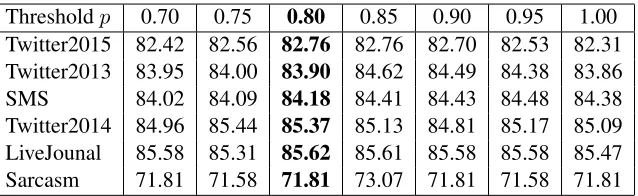
3.1 Subtask A: expression-level sentiment analysis

Thresholdp 0.70 0.75 0.80 0.85 0.90 0.95 1.00 Twitter2015 82.42 82.56 82.76 82.76 82.70 82.53 82.31 Twitter2013 83.95 84.00 83.90 84.62 84.49 84.38 83.86 SMS 84.02 84.09 84.18 84.41 84.43 84.48 84.38 Twitter2014 84.96 85.44 85.37 85.13 84.81 85.17 85.09 LiveJounal 85.58 85.31 85.62 85.61 85.58 85.58 85.47 Sarcasm 71.81 71.58 71.81 73.07 71.81 71.58 71.81

Table 5: The results for subtask A under different thresholdp. Numbers in bold are the submitted results.

3.2 Subtask B: message-level sentiment analysis

We adapted the probability-output weighting ap-proach to subtask B. The experiment result shows that weighting is effective for this subtask. The im-provement using the parameters in Table 3 can be seen from Table 4.

The approach is effective for improving the twit-ter F1 score but degrades the performance on the

Sarcasm data, maybe because it depends too much on the data.

3.3 Experiment analysis

For subtask A, we made iteration stop ati= 2. The reason why there is little improvement is: (1) Af-ter each iAf-teration, the number of new data added to the training data for retraining a new model is rather small. (2) Once the classifier puts a high confidence on a label, this instance is very likely to be similar to existing instances, which means the added instances would not contribute very much to classification.

In the experiments after submission, we tried to interchange the improvement method between the subtasks, but they showed a little decrease on both subtasks. When the model iteration approach was used in subtask B, we did not receive expected im-provement. This may be because that the perfor-mance for subtask B is lower than that for subtask A, which may result in the wrong samples added into the training data. When the probability-output weighting approach was used on subtask A, we only got limited improvement in theF1score.

4 Conclusion

We described our system for two subtasks of Se-mEval 2015 task 10 – Sentiment Analysis in Twit-ter. Our systems are built by integrating a variety of

features into SVM as baselines and then improved by model iteration and probability-output weighting for expression-level and message-level subtasks re-spectively. We compared the results and analyse the reason of the improvement. Our submissions are ranked the 3rd and 2nd among eleven teams on the 2015 test set and progress test set in subtask A and the 7th and 4th among 40 teams on the two test sets respectively in subtask B.

Acknowledgments

We would like to thank the shared task organis-ers for their support throughout this work. This work is partially supported by the National Natural Science Foundation of China (Nos. 11161140319, 91120001, 61271426), the Strategic Priority Re-search Program of the Chinese Academy of Sciences (Grant Nos. XDA06030100, XDA06030500), the National 863 Program (No. 2012AA012503) and the CAS Priority Deployment Project (No. KGZD-EW-103-2).

References

Stefano Baccianella, Andrea Esuli, and Fabrizio Sebas-tiani. 2010. SentiWordNet 3.0: An enhanced lexical resource for sentiment analysis and opinion mining. In

LREC, volume 10, pages 2200–2204.

Chih-Chung Chang and Chih-Jen Lin. 2011. LIBSVM: a library for support vector machines. ACM Trans-actions on Intelligent Systems and Technology (TIST), 2(3):27.

Minqing Hu and Bing Liu. 2004. Mining and summa-rizing customer reviews. In Proceedings of the tenth ACM SIGKDD international conference on Knowl-edge discovery and data mining, pages 168–177. Svetlana Kiritchenko, Xiaodan Zhu, and Saif M.

infor-mal texts. Journal of Artificial Intelligence Research (JAIR), 50:723–762.

Bing Liu. 2012. Sentiment analysis and opinion mining.

Synthesis Lectures on Human Language Technologies, 5(1):1–167.

Yasuhide Miura, Shigeyuki Sakaki, Keigo Hattori, and Tomoko Ohkuma. 2014. Teamx: A sentiment ana-lyzer with enhanced lexicon mapping and weighting scheme for unbalanced data. InProceedings of the 8th International Workshop on Semantic Evaluation (Se-mEval 2014), pages 628–632, Dublin, Ireland, August. Saif M Mohammad and Peter D Turney. 2010. Emo-tions evoked by common words and phrases: Using mechanical turk to create an emotion lexicon. In Pro-ceedings of the NAACL HLT 2010 Workshop on Com-putational Approaches to Analysis and Generation of Emotion in Text, pages 26–34.

Saif Mohammad, Svetlana Kiritchenko, and Xiaodan Zhu. 2013. Nrc-canada: Building the state-of-the-art in sentiment analysis of tweets. In Second Joint Conference on Lexical and Computational Semantics (*SEM), Volume 2: Proceedings of the Seventh Inter-national Workshop on Semantic Evaluation (SemEval 2013), pages 321–327, Atlanta, Georgia, USA, June. Preslav Nakov, Sara Rosenthal, Zornitsa Kozareva,

Veselin Stoyanov, Alan Ritter, and Theresa Wilson. 2013. Semeval-2013 task 2: Sentiment analysis in Twitter. In Second Joint Conference on Lexical and Computational Semantics (*SEM), Volume 2: Pro-ceedings of the Seventh International Workshop on Se-mantic Evaluation (SemEval 2013), pages 312–320, Atlanta, Georgia, USA, June.

Finn Årup Nielsen. 2011. A new ANEW: evaluation of a word list for sentiment analysis in microblogs. In

Proceedings of the ESWC2011 Workshop on ’Making Sense of Microposts’: Big things come in small pack-ages, Heraklion, Crete, Greece, May 30, 2011, pages 93–98.

Olutobi Owoputi, Brendan O’Connor, Chris Dyer, Kevin Gimpel, Nathan Schneider, and Noah A. Smith. 2013. Improved part-of-speech tagging for online conversa-tional text with word clusters. InHLT-NAACL, pages 380–390.

Bo Pang and Lillian Lee. 2008. Opinion mining and sentiment analysis. Foundations and trends in infor-mation retrieval, 2(1-2):1–135.

Hilke Reckman, Cheyanne Baird, Jean Crawford, Richard Crowell, Linnea Micciulla, Saratendu Sethi, and Fruzsina Veress. 2013. teragram: Rule-based de-tection of sentiment phrases using sas sentiment anal-ysis. InSecond Joint Conference on Lexical and Com-putational Semantics (*SEM), Volume 2: Proceedings of the Seventh International Workshop on Semantic

Evaluation (SemEval 2013), pages 513–519, Atlanta, Georgia, USA, June.

Sara Rosenthal, Alan Ritter, Preslav Nakov, and Veselin Stoyanov. 2014. Semeval-2014 task 9: Sentiment analysis in Twitter. InProceedings of the 8th Inter-national Workshop on Semantic Evaluation (SemEval 2014), pages 73–80, Dublin, Ireland, August.

Sara Rosenthal, Preslav Nakov, Svetlana Kiritchenko, Saif M Mohammad, Alan Ritter, and Veselin Stoy-anov. 2015. Semeval-2015 task 10: Sentiment analy-sis in Twitter. InProceedings of the 9th International Workshop on Semantic Evaluation, SemEval ’2015, Denver, Colorado, June.

Maite Taboada, Julian Brooke, Milan Tofiloski, Kim-berly D. Voll, and Manfred Stede. 2011. Lexicon-based methods for sentiment analysis. Computational Linguistics, 37(2):267–307.

Duyu Tang, Furu Wei, Bing Qin, Ming Zhou, and Ting Liu. 2014. Building large-scale Twitter-specific sen-timent lexicon : A representation learning approach. In COLING 2014, 25th International Conference on Computational Linguistics, Proceedings of the Confer-ence: Technical Papers, August 23-29, 2014, Dublin, Ireland, pages 172–182.