An approach to non linear Bayesian forecasting problems with applications

University of Warwick institutional repository: http://go.warwick.ac.uk/wrap

A Thesis Submitted for the Degree of PhD at the University of Warwick

http://go.warwick.ac.uk/wrap/60491

This thesis is made available online and is protected by original copyright. Please scroll down to view the document itself.

An Approach to Non-Linear Bayesian

Forecasting Problems with Applications.

by

Re1io dos Santos MIGON

Thesis submitted to the University of Warwick for the degree

CONTENTS

CHAPTER 1 INTRODUCTION

1.1 - General

1.2 - Outline of Thesis

1.3 - Terminology and Notation

CHAPTER 2 A REVIEW OF DLM AND ARIMA MODELS

2.1 - Introduction

2.2 - Normal Dynamic Linear Model

2.3 - Model Design

2.4

-2.3.1 - Introduction and Definitions

2.3.2 - Similar models and Reparameterization

2.3.3 - Canonical form Models

Constant DLM and Arima Models 2.4.1 - Arima Model

2.4.2 - The State Space Representation

2.4.3 - The Relationship between CDLM and Arima Models

CHAPTER 3 NORMAL DYNAMIC NON-LINEAR MODEL

3.1 - Introduction

3.2 - The Normal Discount Bayesian Model (NDBM)

3.2.1 - Normal Weighted Bayesian Model

3.2.2 - Normal Discount Bayesian Model

3.2.3 - Modified Normal Discount Bayesian Model

3.4

3.5

-Normal Dynamic Non-Linear Hodel

3.4.1 - The Updating Procedure

3.4.2 - Model Summary and Forecasting

3.4.3 - Normal Dynamic Non-Linear Model with Unknown Variance

3.4.4 - A Practical Procedure for Estimating the Observational Variance

The Seasonal Growth Multiplicative Model

3.5.1 - General

3.5.2 - Notation and Definitions

3.5.3 - The Multiplicative Model

3.5.4 - Examples

Appendix 3.1 - General moments for the multivariate normal distribution

Appendix 3.2 - Artificial data generation

CHAPTER 4 AN APPLICATION OF NON-LINEAR BAYESIAN MODELS TO TV-ADVERTISING.

4.1 - Introduction

4.2 - The Advertising Project

4.2.1 - Objectives of the Study

4.2.2 - The Measurements

4.3 - System Model - Basic Assumptions

4.3.1 - Facilities Required

4.3.2 - The Basic Assumptions

4.4 - Dynamic Linear Models

4.4.1 - Introduction

4.4.2 - Broadym Model

4.4.3 - The Local Linear Model

4.5

4.6

-Dynamic Non-Linear Models 4.5.1 - General

4.5.2 - The Assumed Relationship Between Awareness and Advertising

4.5.3 - Notation and Observational Model

4.5.4 - Non-Linear Model with Variable Half Effect

4.5.5 - Non-Linear Model with Fixed Half Effect

Examples

4.6.1 - General

4.6.2 - Examples

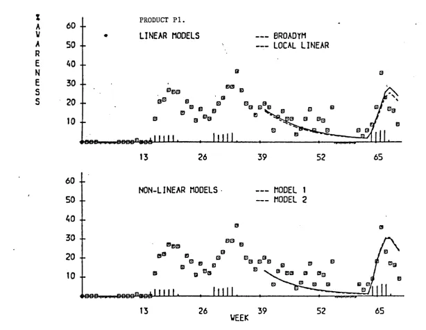
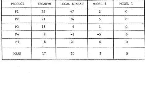
4.6.3 - Comparison

Appendix 4.1 - Memory decay of a population

4.2 - The initial setting for parameters

4.3 - Posterior distribution at the end of the data

4.4 - A comparison of the four models

CHAPTER 5 GENERAL NON-LINEAR MODEL

5.1 - Introduction

5.2 - A Review of Static Generalized Linear Model

5.2.1 - General

5.3

-5.2.2 - The Linear Model for Systematic Effects

5.2.3 - The Genear1ized Exponential Family

5.2.4 - Notation and Some Special Cases

5.2.5 - Comments

Dynamic Generalized Linear Models

5.3.1 - Introduction

5.3.2 - The Model Structure

5.4

-CHAPTER 6

6.1

6.2

6.3

6.4

-CHAPTER 7

7.1

7.2

7.3 7.4

7.5

-General Dynamic Non-Linear Model

5.4.1 - General

5.4.2 - The Guide Relationship

5.4.3 - Updating Recurrence for. the State Vector

5.4.4 - Examples

TRANSFER RESPONSE: MODELLING AND ESTIMATION

Introduction

Transfer Function Modelling and Estimation

6.2.1 - Classical Formulation

6.2.2 - The Box-Jenkins Modelling Procedure

Bayesian Stochastic Transfer Response

6.3.1 - General

6.3.2 - Transfer Response Hodelling

6.3.3 - Stochastic Transfer Response Estimation

Simulation Study

LONG TERM FORECASTING

Introduction

The General Modified Exponential Family of Curves

Characterising the Variation about Trend Curves

The Non-Linear Bayesian Model Applied to Growth Curves

7.4.1 - Trend Plus Random Shock

7.4.2 - The General Model with AR Disturbances

Applications

7.5.1 - General 7.5.2 - Examples

CHAPTER 8 - SUMMARY AND CONCLUSIONS

8.1

8.2

-Introduction

Abstract

This thesis is devoted to the analysis and modelling of time series

and it is concentrated on models and techniques which are of practical value.

In particular we developed a wide class of non-linear dynamic models which

are useful in the handling of real life problems.

Initially we review the basic principles of Bayesian forecasting and

the design of Dynamic Linear Models. The main body of the thesis attacks

the problem of Normal non-linear estimation and forecasting. Some applications

to the seasonal multiplicative model are exhaustively discussed. Following

this we present the results of an application of Bayesian transfer response

in Market Research. This application worked as the very first stimulus to

extend the non-linear models to the exponential family.

Finally we discuss the concepts of stochastic transfer response

modelling and associated sequential estimation, and we report some applications

Acknowledgements.

I should like to express my sincere gratitude to Professor P.J. Harrison

for his efforts in initiating this research, his continuous suggestions, guidance

and general support throughout the period of study.

I am also grateful to Dr. M. West for his discussions and comments and

to Dr. P. Walley for his kindness and attention.

Thanks are also due to Jean Lake, not only for her excellent typing skills,

but for her patience and cheerfulness.

I am deeply grateful to Mirna and the three Musketeers for their patience,

endurance, encouragement and many sacrifices during my period of study.

This research was funded by Conselho Nacional de Desenvolvimento

Cientffico & Tecnologico - CNPq - and I should like to thank the financial

To

Mirna

Marcio

Marcelo

Chapter 1: Introduction.

1.1 General.

This thesis is concerned with the analysis and modelling of time series

and it 1S concentrated on models and techniques which are of practical value.

It· was our decision to develop new models but emphasize the applied and

method-ological aspects of the problem rather than to look for theoretical results.

Time series models can be interpreted as models which are constructed

without drawing on any theories concerning possible behavioural relationship

between variables. This is a distinguishing feature of a time series, as opposed,

say to an econometric model. This field has received an enormous amount of

interest from workers in socio-economics studies, physical and engineering

sciences and in areas such as demography and medicine.

The classical models for time series have been developed since the 40's

and they are based on ARMA processes. A full strategy for time series analysis

was developed by Box and Jenkins in the 70's.

It is worth pointing out that they have started with results of Kolmogorov

and Wiener and are based on the hypothesis of derivable stationarity with

predictors as linear functions of the past observations and mean square error as

criterion of optimality.

The works of Harrison and Stevens (1971, 1976) on Bayesian Forecasting

overcome some of the restrictive hypotheses and opened a very new area for:

practical and theoretical investigation. The approach gives a logically

consistent description of the way in which a forecasting method should deal

with a wide class of situations.

The principle of superposition enables an easy way of building linear models

from separate components, which are structured and facilitates the meaning.

provides a rich and logical framework for mathematical modelling. This is, for

example, the natural way to blend subjective information with data in order to

produce inference. Furthermore, the combination of prior and experimental

information is rigorous and natural.

The Dynamic Linear Models and the Bayesian Forecasting of Harrison and

Stevens have been extended by Ameen and Harrison (1983). The introduction of a

class of Normal Discount Bayesian Models, founded upon the discount concept,

has overcome some difficulties found by practitioners. The innovation or

variance matrix is replaced by a set of discount factors which are invariant to

the measurement scale of the independent and the control variables. This

introduces conceptual simplicity and also removes much of the ambiguity.

The flexibility of these models and their potential as aid to understanding

physical systems as well as forecasting, suggests that more interest will be

centred on their application to diverse fields in the near future.

This thesis is devoted to the examination of a wide class of non-linear

models which, in particular, extends the work of Nelder and Wedderburn (1972)

in Generalized Linear Models. The appropriate sampling distribution should be

used as in West, Harrison and Migon (1983). Some direct application of the

non-linear dynamic models to the estimation of stochastic response is also

discussed.

1.2 Outline of the thesis.

Chapter 2 is concerned with a review of Dynamic Linear Model (D.L.M.)

design and the relationship between constant DLM's and ARIMA models. The main

point is concerned with the design of canonical models which produce desired

forecasting functions. These canonical models can be transformed using similar

linear operators in order to produce a convenient meaningful parametrization.

In Chapter 3 we present a class of non-linear normal dynamic models which

model and reformulates it in order to put forward the non-linear model.

Finally, we present an application to the linear growth seasonal model in a

multiplicative form which avoids transformations and so relates the parameters

in the original measurement scale which is preferred by practitioners.

Chapter 4 consists of a report on an application of Bayesian transfer

response modelling to a marketing problem. At the very beginning of our

study on transfer response, an opportunity to participate in a project involving

the Statistics Department at Warwick University and Millward-Brown Marketing

Research Co. arose. The models developed have been working successfully for

more than two years in their computers and an early practical evaluation can

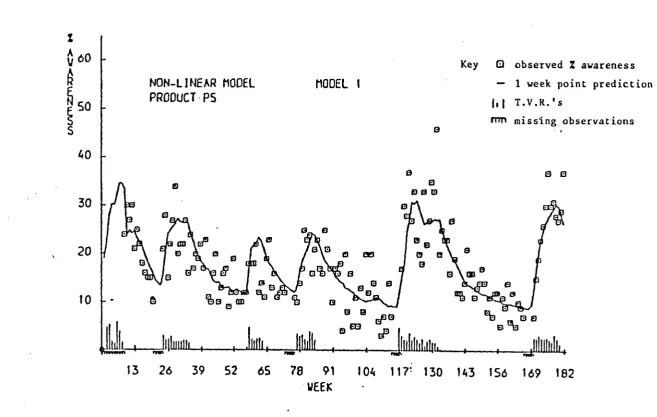
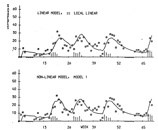
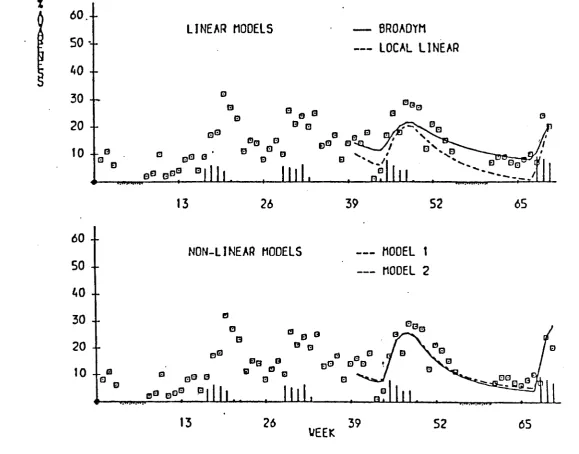
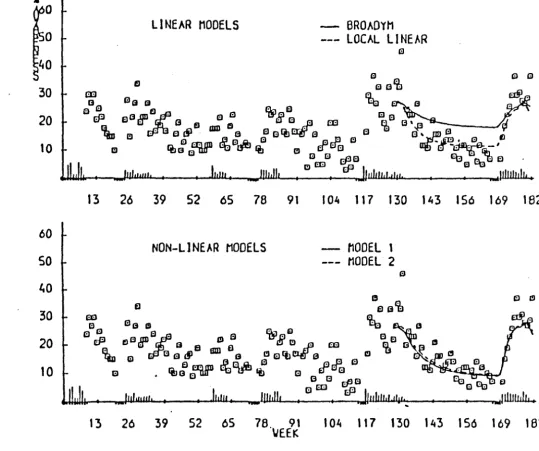
be found in Colman and Brown (1983). Altogether we developed four models, being two linear and two non-linear. The basic linear model is a dynamic extention

of Broadbent's model (Broadbent (1979»). This fortunate application acted as the very first stimulus for the methodological developments presented in this thesis.

An extention of the Normal non-linear models is presented in Chapter 5.

This model can be viewed as a dynamic version of the generalized linear model

of NeIder and Wedderburn (1972).

The linear Bayes approach developed by Hartigan (1969) is extensively used. This method is appropriate to problems of inference when only the first two

moments of the prior distribution and the likelihood are specified. Some

applications for the log-normal and binomial cases are discussed and for

additional applications the paper of West, Harrison and Migon (1983) is recommended.

Chapter 6 considers the on-line estimation of transfer response. The concept

of stochastic transfer response is discussed and some parallels drawn with the

classical approach. The performance of the estimation method was assessed by

a simulation experiment.

forecasting method to the long-term forecasting problem. The low frequency or

trend is represented by a growth curve such as the modified exponential and

the high frequency as an autoregressive process of order p. The parameters are

estimated on-line and it ~s worth pointing out that the principle of superposition

is again used. This method was applied to some real data and the main results

are reported.

The paper of Harrison and Akram (1982) is recommended for a theoretical

discussion of the problem.

1.3 Terminology and Notation

In general we tried to keep the notation as close as possible to other

related works. Throughout the thesis all probability distributions are defined

via densities with respect to Lebesque measure, and they will be represented by

the generic symbol p(.). Some special densities are denoted as:

(i) N8(m,~) is the multivariate normal density of ~, with mean vector

m and variance matrix ~;

(ii) Ge(a,b) is the Gamma density for 8;

(iii) Be(r,s) is the Beta density for e; and

(iv) B(n,p) is the Binomial mass probability function.

The general exponential family has a density given as:

where ~>O and ~ is the natural parameter of the distribution. It includes as

special cases the Normal, Gamma, Poisson and Binomial distributions.

No distinction is made between random variables and their observed value

since, generally, the context will be clear. By x ~ p(.) we mean that x has

multi-variate normal density of x given z; and, in general, (x/z) ~ [~,~J means that

the conditional density is partially specified with mean m and variance matrix C.

All the vectors are underlined, as ~, for example; and matrices appear as

capital letters.

The following abbreviations represent the classes of models discussed in

this thesis.

DLM CDLM

NDLM

NDBM

NWBM

ARlMA

GLM

Dynamic Linear Models;

Constant Dynamic Linear Models;

Normal Dynamic Linear Models;

Normal Discount Bayesian Models;

Normal Weighted Bayesian Models;

Autoregressive integrated moving average models; and

Generalized Linear Models

Finally, it is worth remarking that the equations are numbered according

to the chapters and sections. For example: equation number 4.3.2 means

equation number two in section 3 of Chapter 4. Further notation will be

Chapter 2: A Review of DLM and ARIMA Models.

2.1 Introduction

This chapter is concerned with a review of the Dynamic Linear Model,

model design and the relationship between the class of constant DLM and ARIMA

models.

In Section 2.2 the Bayesian forecasting approach of Harrison-Stevens

(1971 & 1976) is discussed. A more suitable Bayesian formulation is presented. The concept of similar models which is very useful in model design is

introduced in Section 2.3, as well as a strategy to DLM modelling.

Finally in Section 2.4 we show the link between CDLM and ARIMA models.

The Box-Jenkins strategy is briefly discussed and a state space representation

is introduced.

2.2 Normal Dynamic Linear Model

The Bayesian forecasting approach developed by Harrison & Stevens (1976), a reference which we shall abbreviate HS(1976), is based on a complete parametric

description of the process, which is incorporated into a dynamic linear set of

equations describing:

(i) the process observation, and

(ii) the parameter evolution

The parametric structure reduces ambiguity in the model building and so

increases the meaning, which permits communication between the decision maker,

the forecaster and the forecast method in both directions. When building larger

models the forecaster is almost forced into model decomposition, and again

the structure has a great deal to offer.

The dynamics of the system is described by the evolution of the parameters

in time, both as a result of the inherent process and from random shocks as

In its general form the Dynamic Linear Model is stated in terms of an

ordered index which may be regarded as discrete points of time. Such a model

is defined by a quadruple {F,G,V,W} for each time index. The model may then be t

written:

observation equation:

system equation:

where: Y

-t is an mx1 vector

8

-t is an px1 vector F

-t is an mxp matrix

y - t

e

- t of of of

F 8 + \I -t -t -t

G 8 + W - -t-1 - t

observations

parameters at

at time t·

,

time t·

,

independent variables, known at time

G is a known pxp matrix defining the parameter evolution;

'V _{is an mxl vector representing the observation noise;} -t

~ is an pxl vector representing the parameter noise.

(2.2.1)

t;

In general ~ is assumed N(Q'~t) and_w

t is assumed N(Q, ~t) with each being a series of independent random vectors. We should emphasize that the DLM

can be generalized by allowing G to vary throughout the time and by considering

a non zero expected value for 'V and w .

- t - t

An alternative formulation.

Equation 2.2.1 can be rewritten in a more appropriate Bayesian statement for the DLM {F, G, V, W}t,as:

{

observation equation:

parameter relation:

Information

~

Ie

t) '" N[ It

~t; ~t

]

(~tl~t-l)

'"

N[~ ~t-l' ~tJ

(2.2.2)

Definition 2.1: D represents all the available information at t-l. t-l

This includes all available data and subjective information.

However, unless otherwise stated D

t

=

{Dt_l , Yt' It}·

it then follows that given the DLM a future joint forecast distribution can be

obtained for any required time. Further, on reception of the actual observation,

Bayes Theorem can be applied to obtain the posterior parameter distribution

Updating and Forecasting.

The Markovian nature of the model lends itself naturally to a sequential

estimation of -t8 , forecasting future Y k' k~l, and smoothing or filtering, -t+

Le. "forecasting" into the past values of ~t+k' k = -1, -2 ...

The two major operations in the sequential analysis are:

(i) Time update

(ii) Prior to posterior update

where D 1 is as in definition 2.1 and represents all the information up to

t

-and including time t-l.

If p(~tIDt-l) is a N(~~t_l' ~t) then once we observe !t

=

~t' the

parameter posterior distribution at time t is obtained by applying Bayes

Theorem:-L(Yt

I

~t) is the likelihood function. This immediately gives (~tIDt) ~

N(~t' ~t) with the following recurrence relationship for ~t and ~t:

-1

~t

=

R -1 + F' V F --t. - t -:....t - t

m = G m + A e (2.2.3)

- t -t-l - t - t

where as usual in Bayesian Normal Theory e

t Yt - ! t ~~t-l is the one step ahead forecast error and At is the multiple regression vector of ~t on It'

(.!.-A_t !t) R t

or

c

=

R - A Y A' - t - t - t - t - t '

(2.2.4)

where

l t = var(YtID_t_₁)· The latter variance equation together with equation for

~t are often referred to as the Kalman filter recurrence equations [H.S.(1976)].

Forecasting distribution.

The predictive distribution is easily obtained, in an extrapolative way, as

soon as the posterior distribution of the parameter vector

e

at any time - t

t~l is evaluated. The predictions are distributional in nature and derived

from the current parameters uncertainty, future observation noise ~t+k and

the disturbances W k' k=1,2 .•• -t+

From the DLM equation (2.2.1), a future observation variable is written

as:

Y = _F

_e

_{+ '"} -t+k -t+k -t+k -t+k

e

= G

e

+ w

-t+k - -t+k-l -t+k (2.2.5)

Defining

~,t = E(!t+kIDt' !t+k)

~t

= _{var(Q.t+kIDt' .!t+k)}

,

(2.2.6)

C = C are known from the recurrence equations (2.2.3). -0, t - t

Then from (2.2.5) we obtain

~,t

=

G ~-l

,

t

C

=

G C G' + W

~,t - ~-l,t -t+k (2.2.7)

with V k and W k known. _{-t+ -t+}

The prediction mean and variance of the k-steps-ahead process are

written as

and two cases must be considered in order to calculate these values.

Case I: _-t+ F k' k=1,2 ••. known

From (2.2.5) and (2.2.6) we get:

~

with m and

C

obtained recursively for k=1,2 •.• from (2.2.6).

Case II: F k' k=1,2 ••• not known. -t+

(2.2.8)

Let F k be expressed by an expected value F plus a stochastic term

a!,

-t+

where for simplicity we drop the suffix t+k.

Then using a result of Feldstein (1971) we get

~,t

~t

,

F,. t TIl. -r.., -K,t

~

~,t ~,t ~,t

+

~t+k

+ U

where: U

=

(u .. ) is a pxp matrix with elements

1.J

u .. = tr{4J .•

em.

t m.' t +

e,. ]}

1.J 1.J -K, -1<., -r.., t

Finally we would emphasize the basic characteristics of the DLM,

some of which will be largely used in this thesis:

(i) its easy physical interpretation for the parameters, designed

to the requirements of the decision makers;

(ii) its probabilistic information on the parameters at any time;

(iii) its sequential nature which permits a description of systematic changes in the parameters of a system;

(iv) its freedom from stationarity which allows a better description of

"reality", and

(v) its distributional predictive nature.

To complete this section it should be mentioned some new theoretical and

methodological developments in the area of Bayesian Forecasting as the Normal

Discount Bayesian Model [Ameen and Harrison (1983)]; the Generalized Exponential

Weight Regression [Harrison and Akram (1982)]; and the work in robustification

of DLM [West (1981)], the non-normal steady state models of Smith (1979) and

Souza (1981). In the applications of DLM and Bayesian forecasting the papers

of Johnston and Harrison(1980) and Harrison et al (1977) are related with our

2.3 Model Design

2.3.1 Introduction and definitions.

The aims of this section are to show how to design models with a desired

forecast function. The meaning of forecast function is the expected value of

the forecast distribution and it is a local form description of the expected

process trajectory. It is clear that the forecast function is completely

determined by the evolution matrix G, assuming ~+k' k=I,2, ••• known.

A general Normal Dynamic Linear Model is denoted by {!, G, V, ~}t'

with parameterization

e,

where

(e

ID ) ~ N[m , C

J.

Following the same

- - t t - t - t

notational principals a Constant Normal Dynamic Linear Model is {~, ~, V, W}

In order to characterize a class of similar models we have to introduce

the concept of observability. Loosely a deterministic system

is said observable if knowledge of Yt'S over a finite period of time completely

determine the parameter~. Consequently for a constant D.L.M. one can think of

unobservable model as an over-specified model.

Definition 2.1: The deterministic model {~, ~,

Q, Q}

is said to be observable

i f and only i f

1.

=

<!,

!.G, ... F GP-1), is a pxp matrix of full rank p.

The definition 2.1 is extended for a constant Normal DLM {~, G, ~, W}

in a natural way saying that the constant NDLM is observable if the associated

deterministic model is observable.

2.3.2. Similar Models and Reparametrization.

In practice it is very important to transform models in order to get a

meaningful parameterization, so that forecast and information are easily

understood, and subjective knowledge can be incorporated smoothly.

(i) G is similar to

Q.l'

i.e. there exist a full matrix H such that G

₁

= HG

Hl

(ii)

~l

=

!!

~

!!-l ,

=

F H-1

where H ~s a full rank matrix such that H G H-1

= Q.l'

_and

(iii)

!l

Theorem 2.3: Let

e

be the parameterization of the model M and

y

be that of model MI' Suppose that (6 ID ) ~ N[m , C J and (~ ID ) ~ N[m t' C tJ

-t t -t -t -t t -1 , -1 ,

and that M and Ml are similar observable models. Then these models have the same

forecasting function if:

Proof:

!!!.1

,

t

=

- - t ' H ro • with

-1 -1

H

=

T T, T ,exist because Ml is observable

- -1

(';)

_...

_!J.

-1 !!!.1, Gk t = F _ H-L-LH G H k -1J H _mt =

!.

G !!!.t' k :Yk~O

Cii) Because Ml is observable the inverse of !.l exists, and from (i) -1

we can write: T ~

=

2J.

~,t' Then follows that H = ~ T To complete this section we emphasize that having a model

M

with

para-meterization 8 we can reparametrize it through the transformation H: ~~

y,

obtaining the similar model M1

= {!

H-1, H G !!-1, V, H ~ !!-1} with parametrization

it

as stated in Ameen and Harrison (1983).

2.3.3 Canonical form models.

The design of a DLM with some g1ven form to the forecast function, i.e. the

trajectory of the process, can be done in two steps:

(i) write down the canonical design with paramet~ization

!,

and

(ii) reparametrize to any required parametrization, ~

=

g

y,

as discussed in section 2.3.2.

For the model

{!.'

Q.,

~, ~} with parametrization (~tIDt) ~ N(ro , ~t) t

assuming ~+k known, the forecast function

=

F Ok m

- - - t t+k

Using the well known Jordan Decomposition theorem we find a non-singular

matrix~, such that

has p distinctive eigenvalues Xl ••• X

p' and the model

M

is similar to the model

Ml - {!l G₁ ~ ~l}· Hence these models have the same forecast function.

It is not difficult to show that:

=

F H-l Ak

~~t

=

i

_{a. t}

X~

_{, with a. t =}

i=l ~,~ ~, m. ~, t

Now if ~ is of rank p and has r<p distinctive eigenvalues Xl ••• X

p

p

each one with multiplicity p., i=l, ••• ,r, with

~ L p. = p, there exist H

i=l 1

non-singular such that

A. (X.)

1 ~ A. ~ I o ••• 0

o

A. 1. •. 0

1

o

0 O ••• ft..

1:

is a Jordan block of dimension P .•

1

In this case the forecast function is:

=

r

L

i=l

r

=

L P. t (k) X

~

, where P. t

i=O 1, 1 1,

is a polynomial of order p. in k, with degree p.-l.

1 1

Example: A simple cycle is characterized by a pair of distinct eigenvalues

iw -iw .

(e , e ). The model 1n canonical form is completely undesirable since the

the model in canonical form as M

~

{(I ,1);

~

iw

~ -i~;

V, W} with paramet r-ization ~, where (~tIDt) ~ N[~t' ~tJ follows that the forecasting function is:

where:

F (k) = m eiwk t

a .b d

m

=

2"

+

12

an m a ₂ 1

2'

b

- -iwk + m e ,

The forecasting function can be rewritten as:

Ft(k)

=

a cos(kW) - b sin(kw) and it motivates the following model:

- { Ccos (w)

M₁ ::: (1,0); _-S1n . ( ) _w sin(w)l. _{cos (w)J '} V _{, -1 •}

w}

Of course these models are similar and the transformation is defined as:

H

=

~

l

. . =

D

T -1 T.

1 -1 - 1 - The new parametrization is

.it

=

H

e

- - t =

lee

1 , t +

e

2 , t

1

- i

e

1,t 2,t

and

Finally it is worth showing that the forecast function for the model

M

=

{I, ~, ~, w} can be written as a linear function of ~t = (Ft(O) ••• Ft(p-l»)'

Let T

=

(F,

I

G ••• F ~p-l), be of full rank p (the model is observable).

Then Ft(O) ••• Ft(p-l) are linearly independent and Vk>O exist

~

=

(~O"'~P-l)k E ~p such that:

Proof: S

=

T m implies m

- t - - t - t

-1

=

T S.

- t

Hence Ft(k)

=

F Gk T-1

~t

=

~ ~t

p-l

Example:

E ~i,k Ft(i)

i=o

M = {(I,D);

flo

1 llll; V, W} and

(e

ID )

~

N(m ; C ).

T =

n

~)

_,

Gk =

11

kl and St

[Ft(O>] ,

-1

G~

~.

Hence

L9

lJ = T =

F t (1)

Ft(k) F Gk T- 1 S

- - - -t

= F (0) +

k~

(l)-F (08

t t t

=

m₁ t + k m

, 2, t as is well known.

2.4 Constant DLM and ARlMA Models.

2.4.1 ARlMA Models.

Since the developments of Wiener and Kolmogorov in 1940's many studies

have been done based in the hypothesis of stationarity or derivable stationarity,

with predictors as linear functions of the past observations and mean square

error as criterion of optimality.

Box and Jenkins in a series of papers and a book (1976) describe a full

strategy for the construction of linear stochastic difference equations

describing the behaviour of a time series. Briefly, they assume that the

given series Y can be reduced to stationarity by differencing a finite

t

number of times, i.e. by determining the stationary series Z as:

t

z

= (1-B)d Y

t t with d>O integer

and B the backward shift operator in the time index of Y

t' i.e. B Yt

=

Yt-1

An

ARMA

model is assumed for the stationary time series Zt and it is

written as:

where:

(2.4.1)

at' t=1,2 ••• is a sequence of uncorrelated random variables

wi th E

[aJ

=

0 and Y

a (B) = 0

2 _{is the auto covariance}

generating function;

In terms of the original time series we can write:

(2.4.2)

where ~(B) and G(B) are polynomials in B of degree p and q respectively.

These models are the well known ARIMA(p,d,q).

It is worth mentioning the Box-Jenkina procedure to fit a model of the

above form (2.4.2) to a given set of data. It consists of a three steps

procedure:

(i) identification of the order of the model;

(ii) estimation of parameters, i.e. ~'s, e's and 02, and

(iii) a diagnostic check.

These three steps are used iteratively and the popularity of the method

is mainly based in the large quantity of software and relevant literature available.

It is straightforward to show that the mean square error forecast of Y_t+k

from 2.4.2 is its conditional expectation. So rewriting 2.4.2 as ~(B)Yt+k-G(B)at

and taking conditional expectation noting that the conditional expectation

of Y

t , Yt- 1, ••• , at' at-I ••• are their known values at time t, and those for

a

t+k are zero, we get the forecasting as a step by step procedure, taking in turn k=1,2, •.•

2.4.2 The state space representation.

There is a simple and interesting way of obtaining a state space or

Markovian representation for the models described in sec. 2.4.1. The basic

ideas rest on the well known result that any finite order difference or

differential equation can be rewritten as a vector first order equation.

Thus we may rewrite 2.4.2 in an algebraically equivalent form:

e =

G

e

+

r

u

where: 6 is a vector (n+l)xl called the state space vector and _F, C

- t

and

r

are suitably defined matrices.

It should be emphasized that the specific expressions for ~, G and

£

provide merely one way of writing the state space form. Even if we fix the

dimension of

!,

we may still obtain an equivalent state space representation by making a similarity transformation as described in section 2.3.2.

Following Harrison and Akram (1983) a canonical state space representation

for the model:

, where

~(B) and 8(B) are polynomial in B of degree p and q respectively, can be

constructed using:

F = (1,0 ••• 0)

6.=0 if j>q.

J

• G =

La:

1

1

.

, - - n '

° °

max(p,q) and ~.=O if i>p,

1

2.4. The Relationship between CDLM and AR1MA Models.

To complete this chapter we show that any closed Dynamic Linear Model

can be represented as an AR1MA model. The proof of the theorem 2.7 follows from a straightforward application of the following lemmas.

Lemma 2.5: If in the deterministic CDLM, i.e. {!,

Q,

0, O} , the matrix G has eigenvalues A1 ••• A not necessarily distinct nor necessarily non zero then

p

Proof:

P

II

i=l

(l-A. B) Y

=

0

1 t

(l-A_{i B)Yt}

=

_{F[C-A i IJ!t-l and hence}

f(x)

=

P II (X-A.) =

°

is the characteristic equation of G and by the Cayley-1.

i=l

Hamilton theorem f(G) = 0.

Lemma 2.6: Let E be independent identically distributed qxl random vector with - t

zero expectation and let ~. E Rq be (q+l) constant vectors, i=O,l, ••• q. Then

.-:1.

q

Zt

=

L Q" € •

i=l -1. -t-1 (2.4.4)

and cov (Zt' Z )

t-q :f 0, then z t is a Hoving Average Process of order q and can be written

q

Zt e _t + L b. e _t-i' where i=l 1.

the e 's are i.Ld. random variables with zero expectation, and b. 's, i=1,2 ••• p

t 1.

are constants.

A proof of Lemma 2.6 is found in Harrison (1967).

The next theorem shows the representation of a CDLM in the ARMA form.

Theorem 2.7: Given an observable constant DLM

Y =F6 +\1

t - - t t

8

=

G 6 + W

- t - - t - l - t

\I '" [0, V] t

w

t '" [O,,ill

with V>O, dim! = p and G with eigenvalues Al ••• A

p not necessarily distinct nor necessarily non zero

p _P

II (l-A. B) Y = e + L b. e

t .

,

where

i=l 1. t t j=l J -J

the e 's

t are LLd. random variables with zero mean.

Comment: From sections

2.4.2

and

2.4.3

follows that the class of DLM contains the

ARMA class. Since some of the A's can be zero and so can the b.'s, the class

J

Chapter 3: Normal Dynamic Non-Linear Model.

3.1 Introduction

The D.L.M.'s described in the previous chapter provide a comprehensive

framework for the modelling and analysis of a wide class of observed time series.

It is worth pointing out the great flexibility of these models as

components of structural forecasting systems and their potential as aids to

interpreting the observed behaviour of the process.

Although the Dynamic Bayesian Linear Models of HS(1976) have provided

a simple and elegant model formulation and extended the classical models by

offering a reformulisation which includes many facilities which are not

elegantly available in the classical formulation, they have still some

limit-ations.

Indeed, the N.D.L.M. provides a useful approximation to a more general

structure, perhaps after transforming the original data. The problem with

this approach are twofold. First we lose the interpretability of the

parameters, and secondly when transformations are used the requirements of

linearity, constant variance and normality may conflict. In such cases it

is desirable that the appropriate non-normal sampling distribution should be

used, and transformations avoided.

In this chapter we present a class of Normal Dynamic Non-linear Models

which provides a much wider class of applications of the dynamic models to

real life problems. The extension to the general case, i.e. non-normal

In section 3.2 we introduce the Normal Weighted Bayesian Model

[Ameen-Harrison (1983)J, which overcomes some practical

disadvantages associated with Dynamic Linear Models. A discount vector

replaces the DLM system variance matrix; introduces conceptual simplicity;

removes ambiguity and provides a system transition model which is invariant

to the measurement scale of independent and control variables.

As a basis for the development of Normal Non-linear Models in section

3.4, a reformulation of the Normal Discount Bayesian Models is discussed in section 3.3.

Finally, section 3.5 is concerned with the applications of Normal

Non-linear Models. The construction of models is briefly discussed and the discount

concepts used. Some examples of intervention are presented and practical

procedures for estimating the observation variance on-line are discussed; in

particular, slowly changing variances and variance power laws are presented.

3.2 The Normal Discount Bayesian Models (NDBM).

The Normal Dynamic Linear Models presented in chapter 2 require mode1lers

to be familiar with parametric modelling, state space stochastic difference

equations and the Normal probability representation of innovations. The

specification of the associated system variance matrices has proved a major

obstacle in the applications. In general, people have little quantitative

insight for the elements of these matrices. The aim of this section is to

introduce a class of Normal Dynamic Bayesian Models which replaces the

system variance matrix by a set of discount factors.

3.2.1 Normal Weighted Bayesian Model.

A

Normal Weighted Bayesian Model is defined by a quadruple

{F, G, V,

~}t

for each integer t>O. Let D be the available data at time t-l and suppose t-l

that the posterior distribution for

e

~s

Then the model is described by:

(ii) prior distribution:

where:

R

=

H C H' - t - t -t-1 - t

It follows that the predictive distribution is:

where

Further defining e t for !t is:

A

(Y ID _{t t-}1) ~ N[y , _t YtJ

Yt - t - t F G !!!.t-l

Y

t F - t -t -t R F' + V t

= y -y and A = _{R I~/Yt '} t t - t

(~tIDt) ~ N[m , C ]

- t - t

where ~t and ~t may be calculated recursively by

m = G m + A e - t - t -t-1 - t t

C

=

[I-A F ] R

- t - - t - t - t

the posterior distribution

It is worth commenting that the class of Normal D.L.M. is contained in

the class of Normal W.B.M. To see this define

W

=

H C H' - G C G'

-t -t -t-1 -t -t -t-1 -t·

If W

3.2.2 Normal Discount Bayesian Models.

A N.D.B.M. is defined by a quadruple {F, G, V, S} and is a particular

- - - t

N.W.B.M. where always H = B-! G = G' B-!. Interest will be centered on models

-t -t t

-structured such that

Qt = diag{Q.l···~} t has a block diagonal form.

I. - is an identity matrix of dimension p.;

1 1

8.

1 - are

H -t = B

-!

the

G '

- t

=

discount

~

B -!

factors satisfying O<8.~1 ~i=l, ••• p , and

1

the NDBM is obtained.

We have used these ideas in our applications (section 3.5) and a full

account of these models is presented in Ameen and Harrison (1983).

3.2.3 Modified Normal Discount Bayesian Models.

A further class of NWBM's called Modified NDBM's is introduced in this section. The reason for introducing this model class is that there may be a

requirement that the system evolution for the different blocks G. be considered

- 1

as independent of one another. The information from the observation series

Y

t is distributed amongst the components of

!

introducing parameter covariances. However this does not signify that covariances should be developed over time

by discounting or by any other means.

In order to define the modified NDBM consider (~-l/Dt-l) '" N[~t_l ' £t-l]

where, corresponding to any diagonal block structure for G

=

diag{G1 ••• G },

- - - p

at time t-1, the partitioned structure of C is {C •• }, of R is {R •• }.

-t-l -1J - t -lJ for i,j=1,2, ••• p, and B

t = diag{l:p

E.z •••

~}.

Then a modified NDBM {F, G, V,

!l

t defines (~t

I

D t-l) '" N

(2,.

!!!.t-l' !t) where

but R ..

=

G. C •. G! for i;j.

3.3 Reformulation of the DLM.

In order to obtain an extension of the Normal DLM for the non-linear case

we commence by a reformulation of the standard normal analysis.

Suppose we write the NDBM as

(ii) Linear guide relationship: ¢t

= Fe,

where

e

1S a vector of

- t - t - t

the underlying parameters.

(iii) Prior distribution for ¢t given the information up to and including

time t-l

(iv) Finally, the prior distribution for

e

given D

- t t-l

(3.3.1)

If, in addition, we assume that the likelihood of Y

t given ~ and ¢t depends on

e

only through ¢t' then using Bayes theorem we obtain

- t

(3.3.2)

Note that the product of the first two terms in the right hand side of (3.3.2)

is proportional to the posterior density of ~t' so

The posterior density of ¢t has the standard form

r

all

=

r+ V V

On the other hand the second term in the RHS of (3.3.3) is calculated from

the joint prior distribution for (~ ,8 ):

t - t

where:

cov(F

e ; e

In

)

=

F R -t -t -t t-l -t -t

var(F

e In

1)

=

F R F'

-t -t t- -t -t -t

Using the standard Normal theory it follows that the posterior for

e

- t

where:

r' ,..

~t = ~t +

=-

_r [~ _t -ljJ ]

t

~t

=

~t - r' r /r (3.3.4)

Now following West, Harrison and Migon (1983), we show that these updating relations coincide with the Kalman filter equations in the Normal linear case.

First we note that:

where:

r'

= e t + r+ V [y t -Y_{t ]}

- t

Y

t

=

E[Y

t

ID

t-l

]

(3.3.6)

r

Which are the Kalman filter recurrence relations with At

r+V-t

The main conclusions from this sort of analysis, which will help us in the

extension to the non-linear normal case are:

(i) the updating of the distribution of the underlying parameter vector

(ii)

e

follows from the use of Bayes theorem on ~t and from the filtering

- t

back of information via the conditional distribution of _{- t}

e

given

e

and ljit;

-t-l

from equation (3.3.4) it is clear that

e

_-t: depends on D 1 only

t-through the change in the mean of ljit' and similarly C depends only on

- t

D . _t-l through changes in the variance of IjJ • _{t '}

(iii) in the normal case the first and second moments completely characterise

the probability distribution;

(iv) finally the forecast distribution for (YtID t -1) depends on the prior

for !t only through the parameters of (IjJtIDt-l)·

In the coming section we present non-linear analogues for this model where

the prior and posterior for the underlying parameters are only partially

specified in order to obtain a tractable sequential analysis.

3.4 Normal Dynamic Non-linear Model.

Let

e

be a parameter vector with (~t_lIDt-l) _{"" N[mt _1 '£t-l} J, and consider a specified dynamic model, which may be non-linear, applied to this posterior

Let tjJ be a parameter related to

e

through a stated "guide relationship".

g-non-linear,

which may be deterministic or stochastic.

The joint prior distribution for (tjJ ,8 )' is then defined such that: t - t

(3.4.1)

where:

(3.4.2)

Comment: In general the marginal distribution of tjJt does not need to be

normal as we see in chapter 5, even though we consider only the normal

case in this chapter.

In many non-linear models the higher moments of

e

are needed and often we

take the marginal distribution of 8 as normal. In this way we can use the

- t

results about the general moments of products of normal random variables (see

appendix 3.1) in order to use a Taylor expansion including moments of higher

order.

Let the posterior mean and variance of (tjJtIDt) be:

The resulting updating equation derived from (3.4.1) are:

where:

(8

I

D ) 'V N[m ,C ]

- t t - t - t

m - t

h

8 t + _-r' (m-lji ) / r _t

C

=

R - r' _r(r-011)/r

- t - t

3.4.2: Model summary and forecasting

3.4.3

For reference purposes the full system of recursions is summarized here:

(i) observational model

(ii) The guide relationship

(iii) Prior distribution

(iv) Posterior distribution

(v) Underlying parameter updating

h

~

=

~t +

E..'

(m-ljit)/r or ~t

=

!t

+ r' r+V

(vi) Underlying parameter evolution

8 = G m

-t --t-l

!t -~ G C G'

-~

= B B

-t

-

-t-l -t

The predictive distribution for W_{t+k and Yt +k , k>O, for forecasting purposes,}

are available in the following form:

(i) From a practical point of view (Ameen and Harrison (1983») it is most useful to approximate (~t+k/nt) by

(8 _{-t+k t} In) ~ N[mt(k); Rt(k)], _{- -} where:

~(k)

=

Q

~t(k-l), k>O

(3.4.4)

"

(ii) Hence (Wt+k1nt) ~ N[Wt(k); rt(k)]; k>O, where:

"

Wt(O) = W_t and rt(O) = r.

" "

(iii) Finally p(Yt+kln t ) ~ N[Yt(k); Yt(k)], where:

A

wt(k); k>O; and

-3.4.3. Normal Non-linear Model with unknown variance

A simple modification of the model provides a tractable learning procedure

for unknown variance in the normal case. A number of approaches have been

adopted for estimating the observation variance as for example Smith (1977),

Smith and West (1983), Ameen and Harrison (1983).

It is assumed that the variance V

=

~-I

where

~

is an unknown constant. The probability model may be rewritten as:

"-(ii) (wtIDt-l) '" _{N[w t ,} r/~J

. nt-J

, 2J

where the Gamma pdf has the kernel

n

t _1

log¢ 2

-It follows that the recurrence relationships for the updating procedure

and the predictive distribution are exactly as defined in 3.4.2 with the setting

V =1 and: t

(i) Joint prior for (\jJt'~)'

(ii) Posterior distribution for \jJ , ¢ and

e

t - t

(c)

---~

-a + e2 /

t-1 t (r+l)

Note that the point estimates of ~ or l/~ can then be calculated

ex

sequentially; for example

0

2

=

~ is the posterior harmonic

t n

t

mean of the observational variance.

(~IDt ,<p) IV N[~t' ~/~J

( mt

...

=

e

+ r' [m-ljJ

J/r

-t - t

l~

=

R

t - r'r(r-cr )/r2 - - 11

The marginal posterior of

e

can be obtained as a

multi-- t

variate t-student using standard Bayesian analysis.

(d) Finally, the marginal predictive distribution is obtained

from the joint distribution (Y

,¢In)

integrating out

t+1 t

~, given:

3.4.4 A practical procedure for estimating the observational variance.

Although the full Bayesian treatment given in 3.4.3 provides a tractable

learning procedure for unknown observational variance, practitioners would

appreciate some simple but effective robust procedure. In particular, slowly

changing variances and power laws are two important aspects in applications.

A number of approaches have been adopted for estimating the observational

variance, for example Smith and West (1983), Harrison and Stevens (1976),

For a NORMAL DLM (F,G,W,V) , as we have shown in Chapter 2, the predictive

- - - t

" " distribution is (YtID_t

-1) ~ N(yt,Yt), where:

"

Remembering the definition of ~, i.e. ~t

=

!

~'/Yt' it follows that:

"

V

=

[1 - F A Jy

t -t-t t 3.4.5

Using (3.4.5) a simple and effective procedure for variance learning can be

obtained.

an unknown constant V's natural estimate is

where:

x

=

x + d2

t t - l t

n + 1

t - l 3.4.6

In order to robustify the procedure we suggest the practical method:

where k is generally

chosen in the interval [4,6J.

Initial values for (xo,n o) in (3.4.6) may be chosen such that Vo

is a point estimate for V and nO is the accuracy expressed in terms of a number

of degrees of freedom or of equivalent observations.

Cases in which it is suspected that V varies slowly over time, a discount

factor can be introduced so that

Since ¢t has a skew distribution it is wise to choose .95<8<1. Further,

if the initial prior of the parameters vector! is vague, then it is

recommended that variance learning commences at time (p+l) where p is the

vector dimension.

Stevens (1974) g~ves a theoretical basis for the popular empirical variance

law which is often applied in stock control. With positive observations, the

law is:

Empirically a value of b

=

.75 is often appropriate. An estimate of a, at' is then derived from

n

t = 8 n v t-1 + 1 z

t at = _n

t

3.4.8

. f V V -- a"'t+k{E[Y

t+k\Dt]}1' .. 5 Future est~mates 0 are k

t+ If the power is

'" 2b unknown and the variance law written V

t

=

a Yt may be defined

the support for (a,b)

S(a,b\D )

=

S(a,b\D_t ) +

t~

b - loga - 2 b 109;J/2

t -1 2 t

aY t

The best supported values may be used as in Harrison and Pearce (1971).

Ameen and Harrison (1983) recommend that with such a method: '"

d~ = (l-!t~t) min(e~,4 Y

t), S~.98, and that strong prior support must be applied.

It is worth pointing out that in our case F ~s equal to the scalar

- t

r

1 and ~t is just r+ V

t

3.5. The Seasonal Growth Multiplicative Model.

3 • 5. 1 GeneraL

pointed out the importance of the multiplicative model formulation for analysing

seasonal data in forms of separate trend and seasonal components.

Our dynamic non-linear model, when applied to the seasonal growth

multi-plicative case, avoids the inconvenience of transforming the data. The

practitioners may operate with parameters relating to the current level, growth

rate and seasonal effects rather than to transformed mixtures of these

parameters. For example a linear growth on original scale cannot be easily

obtained when a logarithmic transformation is taken - the linear growth

component then produces an exponential growth in the original observations.

Another point we would like to focus on is the often recommended

trans-formation in order to apply stationary time series theory. The work with

X

t =

y~-p,

the transformed series is a clear case of mathematical convenience

leading the modeller to adopt an undesirable model whose meaning is not at all

clear to the decision maker. With the Bayesian approach there is no need to

operate with transformed variables nor to lose interpretability.

Furthermore, it seems to us a quite serious drawback to transfonmed

variables the fact that they may not be robust to departures in the assumptions

on which they are derived. For example if a logarithmic transformation is

taken and a zero or near zero observation occur then the value of x

t =logYt

is

_00.

This means that protection rules need to be introduced to guard against

such occurrences. In general there may be a danger of assigning the much

importance to small values, say at a seasonal trough, compared to the important

values which occur at seasonal peaks.

3.5.2 Notation and Definitions

Let the vector of the underlying parameter ~t be

~

=

[il t '

where:

~t

=

[~lt

and

~

=

(p,oooPr)'

growth; and p ~s the vector of seasonal factors.

The guide relationship is defined as:

where: F

=

(1,0) and ~ (1,0,1,0, ••• ,1,0).

We describe the system evolution by the structure:

(i) systematic evolution - let G be a (T+2) x (T+2) matrix.

where G

~

=

diag{~l; ~2"" '~tTJ

}

- +1

2

d G = [.:os (kw)

an -=1<+1

. -sin(kw)

rTl

=

~

for k=l,2, •.•

L2J;

w T

sin (kw>l

cos (kw)J

3.5.1

(ii) Let B be a (T+2) x (T+2) matrix of discount factors defined as:

B

=

diag{!l; ! 2 " " ' !

rTJ }

LI

+1

where:

matrix of dimension 2, with O<Bi~l, and often B_k+

1

=

B2 for all k=l, •••

[~

3.5.3 The mUltiplicative model.

(i) Observational distribution

h "b ' h l ' d ' d '

were

V

(ii) Prior distribution for 8

- t

Given the information up to and including time t-l,

where:

e

- t

'V

N[m ,C ]

-t-l -t-l

m

=

[ml] and C

-t-l ~2 -t-l

are partitioned to represent the trend and seasonal components.

Let I

=

~ ~t-l ~I be in a corresponding partitioned form. Then

define R ••

-11

-~

-!

B. I .. B. and, for i

I

j, R ..

=

L •. (the modified NDBM).

- 1 -11 - 1 -1J -1J

(iii) Let X

t F - - t IT and U t 1 + - - t H p , then it follows that:

where: x =

!.

~1

u

= H m +1 and - -2

!.

!.II F I ;

=

F R HI

=

V

- -12 21

The joint prior distribution for (~,8) is

- t

where:

=

x u + v

t t 12

r

=

v[~

ID

]

=

V· +v v + v2 +

x

2 v + u2 vII + 2x ~ v_I2

(iv) The updating

(a) The posterior distribution of

W

t is

where:

l/i_t + r

m

=

_r+V e

t, et

t Yt-Yt

all

=

_r_v _{r+V t}

t

and,

(b) The posterior for ~t:

where

3.5.4 Examples

(a) Artificial Data

" m =

e

+ r' [m-'" ]

/r

- t - t - 'l't

c

- t - t R r' r

2. [r-011]/r

For an assessment of the effectiveness of the model an artificial

data series is used comprising 108 months observations. The generating

model, which is described in the Appendix 3.2, combines a linear trend

dynamic model and a 12 period seasonal effect derived from a single first harmonic.

The model is defined as:

sinew)

I}

with w

=

n

cos(w)l '

6

and S

=

diag{Sl I_{z ' SZ} I_{Z}' 61}

=

.99 and Sz

=

.91 and V t A relatively vague prior specification was made:

N[

450.0 10000 0 0

jL

(~IDo) 'V

5.0 0 4.0 _{_ 1 -} which

-0.0 0 I .1 I

1 2

0.0

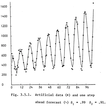
corresponds to a specification of no seasonal pattern! In figure 3.5.1

we can see the observations and the one-step-ahead forecast •

•

1600 1400

•

1200 1000

800

••

600

400

•

•

•

•

•

200

_•

0

0 12 24 36 48 60 72 84 96

Fig. 3.5.1. Artificial data (*) and one step ahead forecast ('V) 8

1

=

.99 82

=

.91.

The performance in terms of the mean absolute desviation (MAD) for each

of the last six years is: year MAD 1 53.8 2 33.3 3 49.7 4 47.0 5 40.9 6 46.0

The observational variance was estimated sequentially given an estimate

of 2510.7. It is worth pointing out that no protection against outliers is

used in the variance estimation.

The final estimates for level and growth are

mean variance

[image:47.581.73.427.201.553.2]

(b) The Turkey Poult Data

The main characteristics of this data set are:

(i) There is clearly a growth in sales over the 10 years and an

annual seasonal pattern.

(ii) Many events, as discussed in Ameen and Harrison (1981) took

place, such as changes in feed price and some promotional

campaigns.

The desirability of incorporating informatiom on these events either by

modelling them or through intervention emphasizes the importance of a flexible

operational system. For illustration purposes an intervention on the level

was made at observation 29. The following seasonal linear growth was applied

to the original data:

F

=

(1,0) H

=

(l,0 ... 1.0), G = diag{G₁···G₆}

B

= diag(B₁I₂; ₈

2 IIO}

~

1]

G

cos kw sin

k~

w rr/6

G _{1 '} ~+l _{• -sin kw} cos kw

,

k .. 1, ••• 6.

The initial information was:

mean variance

level 80 400.0

growth 1.0 .0625

seas. compo 0.0 .18

The power law, with b=l, was estimated on line using a discount factor

B _v

=

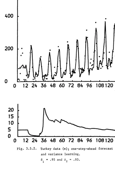
.98

From Fig. 3.5.2 it is evident that, like most practical series, this data

is far from stationarity. Variables such feed price might beneficially be

introduced but they also need to be estimated. Many of the events which

contribute large variation could be anticipated but can only be subjectively

described.

The performance of the non-linear Bayesian model in this case was

quite good. In terms of the MAD for each year we have:

year 6 7 8 9 10 11

MAD 17.5 18.8 21.2 35.7 40.0 23.9*

*This figure is the mean for nine months

The average run length of errors with same sign is 2.16, the MSE for the

last 5 years is 1236.87 and the percentual MAD is 23.5%.

At observation number 29 we drop the level by 30 units and raise the

discount factor to some power in order to represent our extra uncertainty about

the new level. This means that the model is very adaptive with respect to the

trend, and in order to keep the seasonal block unchanged a modified discount

model was used.

Finally it is worth pointing out that the discount factors were not chosen

to optimise a performance criterion but are rounded figures which were thought

400

•

•

•

•

200

•

_•

•

o

o

12 24 36 48 60 72 84 96 108120

20

lS

10

5

o

o

12 24 36 48 60 72 84 96 108120

Fig. 3.5.2. Turkey data (*); one-step-ahead forecast and variance learning.

Sl

=

.95 and ~2

=

.93.

(c) An example of transfer response: Champagne Data.

The main purpose to present this example is the opportunity to

•

introduce an application of transfer response. This data corresponds to the

monthly champaign sales of a French Company, in millions of bottles, from

[image:50.584.140.523.50.626.2]