Development and application of imaging techniques for the investigation of dentinal hypersensitivity

University of Warwick institutional repository: http://go.warwick.ac.uk/wrap

A Thesis Submitted for the Degree of PhD at the University of Warwick

http://go.warwick.ac.uk/wrap/55855

This thesis is made available online and is protected by original copyright. Please scroll down to view the document itself.

Imaging Techniques for the

Investigation of Dentinal

Hypersensitivity

Cara Gail Williams

A thesis submitted for the degree of Doctor of

Philosophy

Department of Chemistry

University of Warwick

Contents

List of Figures... vi

List of Tables... xviii

Acknowledgements ... xviii

Declaration ... xix

Abstract ... xxi

Abbreviations ... xxii

Glossary of Symbols ... xxiii

Chapter 1: Introduction

1.1.1 The Structure of the Tooth: Dentine and Enamel 2 1.1.2 Dentinal Hypersensitivity 3

1.1.3 Treatments for Dentinal Hypersensitivity 4

1.1.4 Sodium Alginate 5

1.2 Microscopy 1.2.1 Optical Microscopy 6

1.2.2 Scanning Electron Microscopy (SEM) 7 1.2.3 White-Light Interferometry 9

1.2.4 Laser Scanning Confocal Microscopy (LSCM) 10

1.2.5 Scanned Probe Microscopy Techniques

1.2.5.1 Atomic Force Microscopy (AFM) 12

1.2.5.2 Scanning Electrochemical Microscopy (SECM) 13

1.3 Dynamic Electrochemistry

1.3.1 Introduction 14

1.3.2 Macroelectrodes vs Ultramicroelectrodes (UMEs) 16

1.3.3 Ultramicroelectrodes: Fabrication 17

1.3.4 Cyclic Voltammetry (CV) 18

1.3.5 Ultramicroelectrode Arrays 20

1.4 Scanning Electrochemical Microscopy (SECM)

1.4.1

1.4.2 Feedback Mode of the SECM 23

1.4.3 SECM: Probing surface topography and activity 26

1.5 Scanning Ion Conductance Microscopy (SICM)

1.5.1

1.6 Carbon as an Electrode Material

1.6.1

1.6.2 Highly Ordered Pyrolytic Graphite (HOPG) 34

1.6.3 Scanning Microcapillary Contact Method (SMCM) 34

1.7 Aims of the Thesis 35

Chapter 2: Experimental

2.1 Preparation of Tooth Surfaces

2.1.1 Dentine Sample Preparation 47

2.1.2 Setup for SECM and LSCM Studies on Dentine 49

2.3 Instrumentation

2.3.1 Cyclic Voltammetry (CV) 53

2.3.2 SECM 54

2.3.3 AFM 54

2.3.4 FE-SEM 54

2.3.5 LSCM 55

2.3.6 SICM 56

2.4 Materials 58

Chapter 3: SECM & SICM Studies of Fluid Flow through

Human and Bovine Dentine, and the Effect of Occlusion Actives

on this Flow

3.1 Introduction 60

3.2 Dentine Structure 68

3.3 Experimental Details 72

3.4 Bulk Examination of Dentine Permeability 75

3.5 Localised Examination of Dentine Permeability using SECM

3.5.1 Results and Discussion: Examination of Redox Mediators 82

3.5.2 Results and Discussion: Effect of Occlusion Actives 87

3.6 Scanning Ion Conductance Microscopy (SICM)

3.6.1 Introduction 92

3.6.1.1 Operating Modes of the SICM 92

3.6.2 Calibration of the SICM 96

3.6.3 SICM Imaging of Dentine 102

Chapter 4: Laser Scanning Confocal Microscopy (LSCM)

Studies of the Permeation of Dentine by Rhodamine B

4.1 Introduction 107

4.2 Experimental Details 111

4.3 Results and Discussion 112

4.3.1 Results and Discussion: Z-Stack Imaging of Dentinal Tubules 4.3.2 Results and Discussion: Time Series Imaging of the Flow of

Rhodamine B through Dentine, and the Effect of Treatments on this Flow

4.4 Conclusions 123

Chapter 5: Localised Dissolution of Enamel

5.1 Introduction 128

5.2 Experimental 129

5.3 Results and Discussion: Analysis of the Etch Pits 131

5.4 Simulations 139

5.5 Conclusions 143

Chapter 6: Carbon as an Electrode Material

6.1 Introduction 146

6.2 Boron-Doped Diamond (BDD) 147

6.3 BDD Microdisc Array: Experimental

6.3.3 Electrical connection to the BDD Microdisc Array 151

6.3.4 Conducting Atomic Force Microscopy (C-AFM) 152

6.3.5 Silver deposition 152

6.3.6 Electrochemical Measurements 153

6.3.7 Laser Scanning Confocal Microscopy (LSCM) 154

6.3.8 Photoluminescence Mapping 155

6.4 BDD Microdisc Array: Results and Discussion 155

6.5 Highly Ordered Pyrolytic Graphite (HOPG)

6.5.1 Introduction 172

6.5.2 Scanning Micropipette Contact Method (SMCM) 173

6.6 SMCM Studies of HOPG: Experimental

6.6.1 Materials 176

6.6.2 Electrical Contact to HOPG 176

6.6.3 Electrochemical Setup 177

6.6.4 Finite element modelling 179

6.7 SMCM: Experimental Results 180

6.8 SMCM: Simulation Results 184

6.9 Conclusions 195

List of Figures

Chapter 1: Introduction

Figure 1.01 The anatomy of the tooth, where i is the crown and ii is the root of the tooth. (a) is the enamel, (b) is dentine, (c) is the pulp, (d) is the gingiva (gum), and (e) is the bone of the jaw. (f) shows the apical foramen, where the blood and nerve supply enters the pulp.

2

Figure 1.02 Schematic showing calcium coordination in the “egg box model”. The dark circles represent the oxygen atoms involved in the coordination of the calcium ion.

5

Figure 1.03 Schematic showing photon and charged particle emission from a surface following electron bombardment. 1 = transmitted electrons, 2 = secondary electrons, 3 = backscattered electrons, 4 = Auger electrons, 5 = absorbed current, 6 = X-rays, and 7 = cathodoluminescence.

8

Figure 1.04 Schematic of a white light interferometer. White light from the light source (1) passes through a collimator (2) before being divided by a beam splitter (3). One beam reflects from the sample (4) while the other reflects from a reference mirror (5). They recombine and pass through an objective lens (6) before being detected by the camera (7).

9

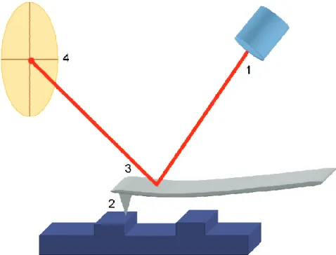
Figure 1.05 The confocal principle. A laser (1) is focused by the objective lens (2) and illuminates the sample (3). Light from the focal place (red) hits the beam splitter (4) and passes through the detector pinhole (5) to the photomultiplier (6). Out-of-focus light (green and blue) is rejected by the pinhole and does not reach the photomultiplier.

11

Figure 1.06 Schematic of the atomic force microscope (AFM). A laser beam (1) is shone onto the cantilever as the tip (2) scans across the surface of the sample. The laser reflects off the back of the cantilever (3) into a photodiode detector (4).

12

Figure 1.07 Processes occurring at the electrode surface. 1: electron transfer at the electrode surface; 2: Surface reactions such as adsorption/desorption; 3: chemical reactions preceding/following electron transfer; 4: mass transport of the redox active from bulk solution to/from the electrode surface.

15

Figure 1.08 Diffusion fields to (i) a macroelectrode, and (ii) a disc UME.

17

Figure 1.09 Typical shapes of cyclic voltammograms obtained at (i) a macroelectrode, and (ii) a UME.

Figure 1.11 Schematic (not to scale) of SECM feedback modes. (i) shows how hindered diffusion leads to negative feedback; (ii) illustrates regeneration of the redox mediator, which leads to positive feedback.

24

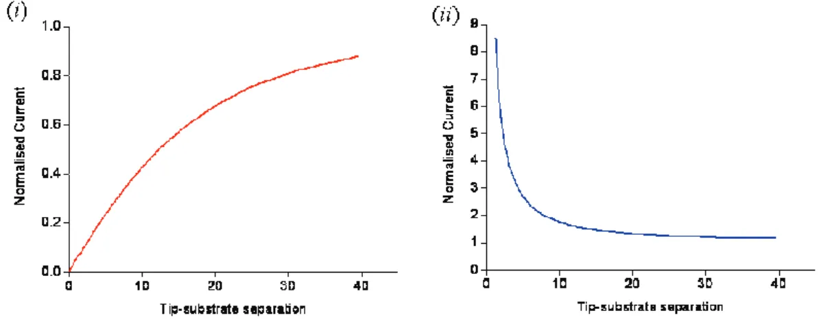
Figure 1.12 Theoretical approach curves for (i) negative feedback and (ii) positive feedback for a 25 µm diameter disc UME.

26

Figure 1.13 An illustration of the varying feedback modes of SECM. The tip is scanned at a fixed height, so the tip-substrate separation, d, and thus the current, changes as the topography of the surface changes (i-iii). Addition of convection to a porous system causes large current increases (iv). The presence of electroactive regions may also be confirmed by large increases in current (v).

27

Figure 1.14 Schematic showing the interaction of diffusion fields in the SG-TC mode of SECM.

28

Figure 1.15 Schematic showing the SICM experimental set-up. A micropipette tip containing an intra-pipette Ag/AgCl reference electrode (1) is filled with an inert electrolyte solution, as is the reservoir (2). A second Ag/AgCl reference electrode (3) sits in the reservoir and a potential is applied between the two electrodes. The magnitude of the resulting migration current that flows is dependent on the distance between the tip and the sample (4).

30

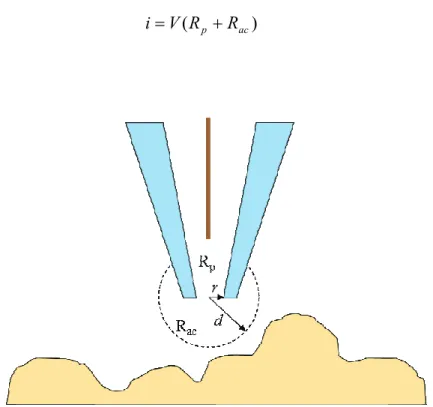
Figure 1.16 Schematic showing the resistances associated with the SICM technique. Rp is the resistance of the pipette

opening; Rac is the access resistance of the pipette. r is

the radius of the pipette and d is the tip-substrate separation.

31

Figure 1.17 (1) Schematic showing grain structure of a polycrystalline diamond film. (2) Differential boron uptake in different grains is indicated by dark and light regions. (3) The sample is processed to remove the growth and nucleation surfaces. (4) Resultant sample for investigation; note the complex interconnection of grains with different dopant densities.

33

Chapter 2: Experimental

Figure 2.01 Schematic displaying the location from which the occlusal and root discs are taken

48

Figure 2.02 Photograph showing the SECM experimental set-up. 50 Figure 2.03 Images obtained using optical microscopy showing (i)

a side view of a 10 µm diameter Pt UME, and (ii) an end-on view of the same Pt UME.

53

Figure 2.04 Schematic showing the experimental set-up for all

Chapter 3: SECM & SICM Studies of Fluid Flow through

Human and Bovine Dentine, and the Effect of Occlusion Actives

on this Flow

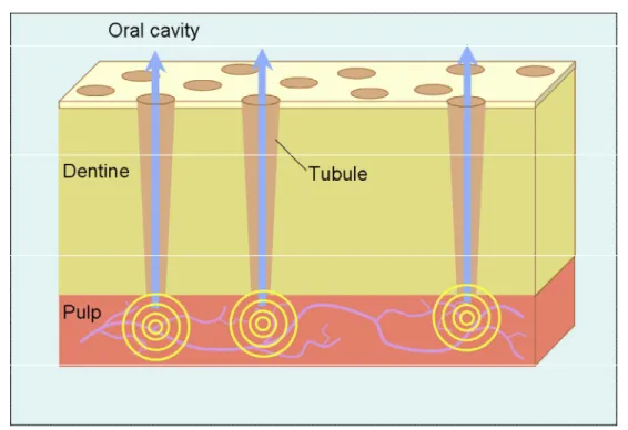
Figure 3.01 Schematic to demonstrate the hydrodynamic theory of dentinal hypersensitivity

59

Figure 3.02 Schematic showing the set-up used for hydraulic

conductance measurements. 63

Figure 3.03 Optical image of bovine dentine showing dentinal tubules. Scale bar represents 10 µm.

69

Figure 3.04 Contact-mode AFM height image showing tubule diameters of 2.61 and 1.94 μm and surface roughness of the order of 500 nm for a bovine dentine sample.

70

Figure 3.05 FE-SEM images of bovine dentine. Scale bar

represents (i) 20 μm and (ii) 5 μm. 71 Figure 3.06 FE-SEM images of bovine dentine. (i) shows the

thickness of the dentine slice (ca. 82 μm); (ii) is a higher resolution image of a region from (i), and shows microtubules (indicated by the red squares) branching normal to the pulp-enamel direction, indicated by the double-headed arrow. Scale bar represents (i) 20 μm and (ii) 2 μm.

71

Figure 3.07 A typical CV recorded using a 25 µm diameter Pt UME in a 5 mM solution of IrCl63-, containing 0.1 M

KNO3 as supporting electrolyte. Also present in

solution were HEPES buffer (20 mM) and CaCl2 (1

mM). The observed limiting current (~27 nA) is slightly higher than the expected current from theory (19.78 nA, applying a diffusion coefficient for IrCl6

3-of 8.2 × 10-6 cm s-142 ); this is probably due to a very slight error in preparing the solution (the observed current would be obtained if the solution had a concentration of 5.0001 mM).

73

Figure 3.08 A plot showing an experimental approach curve to an insulator (black) fitted to a theoretical approach curve (red) for a 25 µm diameter tip UME with RG = 10.

74

Figure 3.09 Plots of pressure vs time showing the difference in the pressure increase for dentine discs of different thicknesses.

76

Figure 3.10 Plots of pressure vs time showing the difference in the pressure increase for dentine discs etched with 3% citric acid for different time periods.

77

Figure 3.11 Plots of pressure vs time showing the difference in the pressure increase for untreated dentine compared with dentine treated with 3% alginate gel. The flow solution was 1 mM CaCl2.

electrolyte. 1 mM CaCl2 was also present in the

solution. CVs were run at a scan rate of 10 mV s-1. Increasing amounts of 3% alginate gel were added in 0.5 cm3 aliquots; black: 0 cm3 added; red: 0.5 cm3 added; dark yellow: 1 cm3 added; blue: 1.5 cm3 added;

purple: 2 cm3 added.

Figure 3.13 Pressure-time profile recorded for flow of Ru(NH3)63+

through dentine over 66 minutes. 83 Figure 3.14 Current images for the diffusion controlled reduction

of Ru(NH3)63+ as a tip UME is scanned over the

dentine surface. (i) is the image obtained with no flow, and (ii) with 3 ml/hr flow, both in the absence of Ca2+. (iii) and (iv) were both obtained in the presence of Ca2+, and are images acquired with no flow and 3 ml/hr flow respectively. The tip UME (a = 12.5 μm) was initially positioned at a distance of 7μm from the surface. The image was recorded with a tip scan rate of 10 μms-1_.

84

Figure 3.15 i-t transient measured for Ru(NH3)63+ over a 20 minute

period with the tip held at a diffusion-controlled potential.

85

Figure 3.16 i-t transient measured for ferrocenemethanol over a 30 minute period

86

Figure 3.17 Large scan current images for the diffusion-controlled oxidation of IrCl63- as a tip UME is scanned over the

dentine surface. (i) is the image obtained with no flow, and (ii) with 3ml/hr flow. (iii) is the image obtained on subtraction of (i) from (ii), i.e. the image due to convection only. The tip UME (a = 12.5 μm) was initially positioned at distance of 7 μm from the surface. All images were recorded at a tip scan rate of 10 μm s-1.

88

Figure 3.18 Pressure-time profile recorded for flow of IrCl63- at a

flow rate of 3 cm3 hour-1 through dentine over 90 minutes.

89

Figure 3.19 Series of SECM images showing it/i∞ for: (i) a dentine sample with no applied pressure; (ii) the same sample after application of a pressure of 2 kPa using a gravity feed system; (iii), (iv) and (v) the same sample after 1, 2 and 3 applications, respectively, of a paste containing 3% alginate gel as a candidate active for dentinal hypersensitivity.

91

Figure 3.20 A typical SICM approach curve to a glass substrate for a 4 µm diameter micropipette, where the tip current is normalised with respect to the bulk current and plotted against the tip-substrate separation (d) expressed in tip radii (r). In this case r=2 μm. The micropipette and reservoir were both filled with 0.1 M NaCl. 2 Ag/AgCl electrodes served as the reference electrodes within the micropipette and in the reservoir.

Figure 3.21 Schematic diagram representing the resistances associated with the micropipette, where Rp is the

resistance due to the micropipette and Rac is the access

resistance of the micropipette aperture.

94

Figure 3.22 Schematic demonstrating the effect of tip oscillation on the tip current. (i) shows the effect of oscillating the tip when it is positioned far from the surface; (ii) exhibits the effect on tip current when the tip is close to the surface.

95

Figure 3.23 Figure to compare the response of the AC current (blue) and the DC current (red) for a 4 μm micropipette tip over the same approach distance (7 μm). The magnitude of the AC current (ie the first harmonic amplitude of the DC current) was measured from peak-to-peak (p2p).

96

Figure 3.24 (i) Optical and (ii) SICM image (micropipette diameter 1 µm) showing a substrate consisting of bands 5 µm in width, separated by 20 µm, that are raised 0.5 µm from the plane. The xy scale bar in both images represents 25 µm; the z scale bar for the SICM image (ii) runs from 0 (black) to 0.5 (white) µm.

97

Figure 3.25 SICM images of the raised band structure on silicon wafer, recorded with a 3.5 μm diameter micropipette under feedback utilising the first harmonic, with two different set-points. The tip was oscillated over 40 nm at a frequency of 80 Hz. The substrate had band width 5 μm and band height 0.5 μm, with a 20 μm repeating pattern. (i) and (ii) are images recorded over the same 100 × 50 μm area, with the set point of (i) approximately 0.85 μm closer to the surface than the set-point for (ii). (iii) shows the average cross section in the direction normal to the bands for (i) black and (ii) red. Lines have been shifted so that the flat areas between bands match approximately.

98

Figure 3.26 SICM image of a calibration grid consisting of 5 µm × 5 µm squares raised 180 nm from the plane. The image was recorded using a 1 μm diameter tip filled with 0.1 M NaCl. The reservoir was also filled with 0.1 M NaCl. The tip was oscillated over 40 nm at a frequency of 80 Hz. The xy scale bar represents 10 µm; the z scale bar runs from 0 (white) to 185 (black) nm.

99

Figure 3.27 Images of a calibration grid, 10 μm pitch, 180 nm depth, recorded using contact-mode AFM (i) and (ii) or and SICM (1 μm diameter pipette) (iii) and (iv). (ii) and (iv) are cross-sections of the 2-dimensional images taken from (i) and (iii), respectively. Curves in (iv) have been offset from one another in the vertical

as it scans over a step at two different set points (d1>d).

Figure 3.29 Schematic showing the path of ion flow as a pipette is positioned above a pit, either (i) offset or (ii) coaxially over a pit.. The weight of the arrow is demonstrative of the relative magnitude of the ion flux out of the pipette. NB: there will be a net flow equal and opposite to this to balance the charge.

101

Figure 3.30 An SICM image of dentine recorded using a 3µm diameter micropipette containing 0.1 M NaCl. The tip was oscillated over 40 nm at a frequency of 80 Hz.

102

Chapter 4: Laser Scanning Confocal Microscopy (LSCM)

Studies of the Permeation of Dentine by Rhodamine B

Figure 4.01 LSCM images of human dentine at (i) an excitation wavelength (λex) of 543 nm. Note there is very little

autofluorescence of dentine. (ii) On dipping the dentine into 10 μM Rhodamine B solution, the tubules become visible. (iii) At λex = 488 nm (i.e. λex for

fluorescein), dentine was seen to autofluoresce. (iv) On dipping the dentine into 10 μM fluorescein solution, the tubules become less apparent as it becomes more difficult to differentiate between them and the dentine background. The scale bar represents 20 µm in all images.

113

Figure 4.02 z-stack at 543 nm of human dentine. A section in the x-axis (*) shows the tubules are all of a similar diameter over the 20 μm stack

114

Figure 4.03 A selection of LSCM images marking the flow of rhodamine B through dentinal tubules for brushed dentine. Blue regions indicate low fluorescence; red regions represent high fluorescence. Image acquisition was started concurrently with the flow. The time indicated in the corner of each frame refers to the time at which that frame began to be recorded (~6 s image duration). The scan direction is indicated by the arrow. Images were recorded continuously in the plane parallel to, and just above, the substrate surface over a time period of 2 minutes. Each frame shows a region 460 μm x 460 μm, and the scale bar denotes 100 µm. Inset: Pressure-time data obtained during the imaging measurement (average of 4 runs).

116

Figure 4.04 Pressure-time data obtained during fluid flow through human dentine, etched in 10% citric acid, after: (a) no further treatment; (b) treatment with a commercial varnish (Cervitec®). Each plot shows the mean pressure observed for 4 fresh dentine samples.

Figure 4.05 Optical DIC micrographs of: (a) untreated dentine; and (b) dentine treated with a commercial varnish (Cervitec®) at a magnification of x200.

118

Figure 4.06 A selection of LSCM images showing the flow of rhodamine B through dentinal tubules for dentine treated with alginate paste. Black regions indicate low fluorescence; white regions represent high fluorescence. The scan was started concurrently with the flow. The time indicated in the corner of each frame refers to the time at which that frame began to be recorded. The scan direction is the same as for Fig. 2. Images were continuously recorded in the plane parallel to the substrate surface over a time period of 2 min. Each frame shows a region 460 × 460 μm. Scale bar: 100 μm. See text for description of processes occurring.

120

Figure 4.07 Black squares: Pressure–time data obtained during fluid flow through human dentine, etched in 10% citric acid, after brushing with a placebo paste. The plot shows the mean pressure observed for 4 fresh human dentine samples. Red triangles: Pressure–time data for fluid flow through human dentine, etched in 10% citric acid, and then brushed with alginate paste average of 4 data sets). The error bars for the alginate data are larger.

121

Chapter 5: Localised Dissolution of Enamel

Figure 5.01 A schematic showing the localised dissolution process. 131 Figure 5.02 An optical micrograph showing a series of etch pits

separated by 250 μm centre-to-centre. Scale bar represents 100 µm.

132

Figure 5.03 A typical set of interferometry images showing (a) a 2D view of the surface, (b) the diameter of the pit, and (c) the depth of the pit.

133

Figure 5.04 Plot showing the change in etch pit diameter with increasing experiment time. The etch solution contained 0.1 M KNO3 only. Etching was achieved by

applying a constant current of 50 nA.

134

Figure 5.05 Plot of the etch pit depth with etching time. The etch solution contained 0.1 M KNO3 only. Etching was

achieved by applying a constant current of 50 nA.

135

Figure 5.06 Plot showing the amount of material lost with increasing experiment time. The etch solution contained 0.1 M KNO3 only. Etching was achieved by

applying a constant current of 50 nA.

presence of sodium L-lactate at a concentration of 50 mM.

Figure 5.08 Plot showing the increase in pit volume with increasing etching time, in the absence (black squares) and presence (red circles) of 50 mM sodium L-lactate.

138

Figure 5.09 The effect of NaF treatment on etch pit development, as a function of etch time. The black squares represent the volume of the pits formed in the absence of NaF, while the red circles show the volumes for a surface treated with NaF.

139

Figure 5.10 Simulation domain for the axisymmetric cylindrical geometry used to model the formation of etch pits in dental enamel.

140

Figure 5.11 Plot showing experimental (black squares) and simulated (red circles) pit volumes in an etching solution containing only 0.1 M KNO3. A rate constant

of 0.3 cm s-1 was applied in the simulations.

142

Chapter 6: Carbon as an Electrode Material

Figure 6.01 Schematic showing the fabrication process for the BDD microdisc array

150

Figure 6.02 (i) is a photoluminescence (PL) image showing approximately 78 BDD microdisc electrodes. (ii) is a FE-SEM image of the same microdisc array after electrodeposition of silver from a solution containing 1 mM AgNO3 in 0.2 M KNO3. A deposition potential of

-0.2 V (vs Ag/AgCl) was applied for 60 s.

156

Figure 6.03 Cyclic voltammograms for the reduction of 10 mM Ru(NH3)63+ (in 0.1 M KCl) at the BDD microdisc

array at scan rates of 5 (lowest peak current), 10, 20, 50 and 100 (highest peak current) mV s-1-.

157

Figure 6.04 Cyclic voltammograms for the reduction of 0.1 mM Ru(NH3)63+ (in 0.1 M KCl) at the BDD microdisc

array at scan rates of 5 (lowest peak current), 10, 20, 50 and 100 (highest peak current) mV s-1-.

158

Figure 6.05 Simultaneously recorded C-AFM (i) height and (ii) conductivity images, recorded at a tip potential of -2.5 V with a 10 MΩ current limiting resistor in series, of a typical BDD microdisc electrode in the array.

160

Figure 6.06 Current – voltage curves recorded with the C-AFM tip held stationary in (i) a high conductivity region, and (ii) a low conductivity region of the BDD microelectrode shown in Figure 6.05. The solid and dashed lines represent repeat measurements recorded

in the same zone. Note that no current limiting resistor was present during these measurements.

Figure 6.07 500 μm × 500 μm SG-TC SECM image recorded for the collection of Ru(NH3)62+ electrogenerated from 5

mM Ru(NH3)63+ (in 0.2 M KNO3) at the surface of the

BDD microdisc array. The substrate potential was maintained at -0.4 V, whilst the 25 μm diameter Pt UME tip was maintained at 0.0 V. A tip-substrate separation of ca. 10 μm was employed during imaging

164

Figure 6.08 100μm × 100 μm SG-TC SECM images of an individual BDD microdisc in the array at substrate potentials of: (i) -0.4 V; (ii) -0.3 V; and (iii) -0.2 V. The 5 μm diameter Pt UME tip was held at a constant bias of 0.0 V, thus enabling collection of surface-generated of Ru(NH3)62+ from 5 mM Ru(NH3)63+ (in

0.2 KNO3) at a diffusion-controlled rate. A

tip-substrate separation of ca. 0.6 μm was employed.

165

Figure 6.09 SG-TC images of a second individual BDD microdisc electrode in the array at substrate potentials of: (i) -0.4 V; (ii) -0.3 V and (iii) -0.2 V. The experimental conditions were as for Figure 6.08, except that a tip-substrate separation of ca. 1 μm was employed.

167

Figure 6.10 Feedback approach curves recorded in the zones of high activity for the two BDD microdisc electrodes shown in Figure 6.09 (●) and 6.10(●). For all measurements, the tip was held at -0.4 V and the substrate was maintained at 0.0 V in a solution containing 5 mM Ru(NH3)63+ in 0.2 M KNO3. the solid

line is the theoretical current response for positive feedback.

168

Figure 6.11 FE-SEM images of two different electrodes within the microdisc array (electrode 1: images (i) and (ii); electrode 2: images (iii) and (iv)) after electrodeposition of Ag (60 s electrodeposition time from a solution containing 1 mM AgNO3 in 0.2 M

KNO3). Two detectors were used: (1) a conventional

SE2 detector; and (2) a high efficiency in-lens detector. The former allowed location of the Ag particles, (i) and (iii), whereas the latter allowed simultaneous imaging of the grain structure and Ag particle morphology, (ii) and (iv).

169

Figure 6.12 A selection of LSCM images of the pH-dependent fluorescence profile of fluorescein at the BDD microdisc array after application of a potential of -1.4 V in a solution containing 0.2 KNO3 and 10 μM

fluorescein, resulting in the local increase of the pH due to reduction of oxygenated water. The scan was started immediately after stepping the potential. The

parallel to the microdisc array surface over a time period of 28 s. The scale bar in the frame represents 100 μm.

Figure 6.13 Schematic showing the crystal structure of HOPG. 172 Figure 6.14 Schematic showing the principle behind the Scanning

Micropipette Contact Method (SMCM).

177

Figure 6.15 Optical image showing a 300 nm diameter micropipette approaching the HOPG surface. Scale bar represents 500 μm.

178

Figure 6.16 Typical tapping mode atomic force microscopy (AFM) images of ZYA grade HOPG. Scale bar 1 μm, height range 0 - 5 nm. (i) shows a region with a step density of 0.2 µm/µm² ; (ii) shows a region with a step density of 0.7 µm/µm².

180

Figure 617 Plot to show the fit between experimental (black) and simulated (blue and red) cyclic voltammograms for a micropipette with rp = 225 nm. The solution was FA+ (2 mM) with 0.1 M NaCl. The arrow indicates the direction of the scan. A clear fit is seen to Nernstian kinetics.

181

Figure 6.18 Linescans to show the current generated when the half-wave potential was applied at a series of points across the HOPG surface, using (a) FA+ or (b) Fe(CN)64- as

the redox mediator.

182

Figure 6.19 Plot showing a series of cyclic voltammograms recorded at consecutive points on the HOPG surface for a 550 nm diameter micropipette. Three CVs were recorded at each position. The scan rate was 150 mV s-1. The arrow indicates the direction of the scan.

183

Figure 6.20 Simulation domain for the axisymmetric cylindrical geometry used to model the micropipet system: (i) the full geometry for a uniformly active surface; and (ii) the modification when the substrate is partially active.

185

Figure 6.21 Plot of simulated data demonstrating how the steady state diffusion-limited current (normalised as described in the text) at a 1 μm radius micropipette (l = 400 µm, γ=7.5°, c*=2 mM, D = 6 ×10-6 cm2 s-1) is affected by the meniscus radius, a.

189

Figure 6.22 Plot of simulated data demonstrating how the steady state diffusion-limited current (normalised as described in the text) at a 1 μm radius micropipette (l = 400 µm, γ=7.5°, c*=2 mM, D = 6 ×10-6 cm2 s-1) is affected by the meniscus height, h.

190

Figure 6.23 Simulated cyclic voltammograms at scan rates of 20, 50, 100, 200, 500 and 1000 mV s-1 for Nernstian ET at a 1 μm radius micropipette (a=800 nm, c*=5 mM, h=200 nm, γ=7.5°). The arrow indicates the direction of the scan.

191

Figure 6.24 Simulations showing the effect of kinetics on the shape of cyclic voltammograms. Black: Nernstian response.

Red: k0 = 0.1 cm s-1. Green: k0 = 0.01 cm s-1. Blue: k0 =

0.001 cm s-1. Scan rate 100 mV s-1. The concentration of electroactive species was 5 mM, with rp = 1µm, a = 800 nm, h = 200 nm, and l = 400 µm. The arrow indicates the direction of the scan.

Figure 6.25 Simulated concentration profile within a micropipette where rp = a = 500 nm, c* = 2 mM, h = 100 nm, and l = 0.4 mm. The contour line on the magnified image shows 95% concentration.

193

Figure 6.26 Simulations showing the voltammetric responses of (i) a uniform surface with Nernstian response (red) and Butler-Volmer (black) kinetics with k0 = 0.5 cm s-1;

compared with (ii) a surface containing a 1 nm width step defect (see Figure 3 for geometry). In this latter situation the data are for Nernstian ET (red) and Butler-Volmer kinetics (black) with k0 = 0.5 cm s-1

inert basal plane. A 580 nm diameter micropipette containing 2 mM redox active species (D = 6 × 10-6

cm2 s-1) was simulated. The arrows indicate the direction of the scans. Horizontal line to aid comparison.

List of Tables

Table 2.01 Grades and suppliers of all chemicals used in the studies described within this thesis.

58

Table 3.01 Summary of results from CV experiments on the effect of adding 0.5 cm3 aliquots of 3% alginate gel to a 5 mM Ru(NH3)63- solution in the presence of 1 mM

CaCl2. The solution also contained 0.1 M KNO3.

81

Table 5.01 Boundary conditions for finite element modelling. 141

Table 6.01 The boundary conditions for the simulation of the voltammetric response of a micropipette in the contact method.

Acknowledgements

Firstly I would like to thank Prof. Julie Macpherson for all her help, patience and guidance throughout my PhD, and for seeing potential in me (no electrochemistry pun intended) when I really couldn’t see it myself. Many thanks also to Prof. Pat Unwin, for sharing his knowledge and his ever-present optimism, even when things weren’t going so well. Huge thanks must also go to Charlie Parkinson at GSK for all his support and enthusiasm during my PhD and for giving me a fantastic insight into industry.

Thanks to Sara Dale for being my singing partner in the office and a great ear to sound off to when things got hard, and to Anna Colley for her constant stream of gossip and for being a fantastic running partner. Special thanks also to Martin Edwards - your patience knows no bounds, even when I’m having my dimmest moments. You’ve helped me more over the past few years than I could even begin to tell you, and I really appreciate it. Plus of course you introduced me to Quean’s, and my palate is indebted to you for that.

To my fellow members of the C111 crew (massive), thanks for helping the days to go quickly whether experiments were going well or otherwise. To all the members of the Electrochemistry and Interfaces group, past and present, I wouldn’t have changed the past four years for anything – thank you.

Thanks must go to Neil Wilson for helpful discussions, and even the odd chocolate biscuit here and there. Thanks to Steve York for his guidance on FE-SEM and not getting annoyed when I was just forgetting something simple. Thanks to Marcus Grant and Lee Butcher for all their help with my rig setup requests, and for the frequent comic interludes. Many thanks to Peter Brindley for the enormous number of SECM cell bodies he made over the duration of my PhD.

Declaration

The work contained within this thesis is entirely original and my own work,

except where acknowledged. I confirm that this thesis has not been submitted for

a degree at another university. All Comsol simulations were developed by Martin

Edwards. All work on boron-doped diamond was carried out in conjunction with

Anna Colley. SMCM and SICM work was carried out with the help of Martin

Edwards. AFM images of HOPG were recorded by Manon Guille.

Parts of this thesis have been published as detailed below:

“Examination of the Spatially Heterogeneous Electroactivity of Boron-Doped

Diamond Microarray Electrodes”, A. L. Colley, C. G. Williams, U. D'Haenens

Johansson, M. E. Newton, P. R. Unwin, N. R. Wilson, J. V. Macpherson, Anal.

Chem. 2006, 78(8), 2539-2548.

“Laser Scanning Confocal Microscopy Coupled with Hydraulic Permeability

Measurements for Elucidating Fluid Flow across Porous Materials: Application

to Human Dentine”, C. G. Williams, J. V. Macpherson, P. R. Unwin and C.

Parkinson, Anal. Sci., 2008, 24, 437–442.

“Scanning Micropipet Contact Method (SMCM) for High Resolution Imaging of

Electrode Surface Redox Activity”, Cara G. Williams, Martin A. Edwards, Anna

“A Realistic Model for the Current Response in Scanning Ion Conductance

Microscopy (SICM) and Implications for Imaging”, Martin A. Edwards, Cara G.

Abstract

The overall aim of this thesis is to examine the underlying physical basis of dentinal hypersensitivity and to assess methods of treating this cause using imaging techniques. The scanned probe microscopy (SPM) techniques are then extended to the study of carbon-based electrode surfaces, as described in the final chapter.

The use of scanning electrochemical microscopy (SECM), combined with in situ pressure-time measurements, is described as a means to investigate the flow of fluid through human and bovine dentine, and the subsequent effect of occlusion treatments on this flow. Scanning Ion Conductance Microscopy (SICM) is also introduced as a technique for imaging dentine, with instrument design and development described, and also calibration of the technique.

Laser scanning confocal microscopy (LSCM) coupled to a constant volume flow-pressure measuring system is introduced as a new technique for the quantitative measurement of fluid flow across porous materials. The methodology described herein firstly allows a ready assessment of the general efficacy of treatments via hydraulic permeability measurements. Second, LSCM images allow the nature of the flow process and the mode of action of the treatments to be revealed at high spatial resolution. For the particular case of dentine, we demonstrate how the method allows candidate treatments to be compared and assessed.

To complement the studies into dentinal hypersensitivity, microscopic dissolution of bovine enamel is investigated. This chapter describes a novel approach, based on SECM, to promote the localised dissolution of bovine enamel, effected by the application of a proton flux to the enamel surface from a UME positioned within 5 μm of the surface, in aqueous solution. The approach results in a well-defined “acid challenge” yielding well-defined etch pits that were characterised using light microscopy and white light interferometry. The effect of etching in the presence of lactate is considered, as is the effect of treating the enamel samples with sodium fluoride prior to etching. The approach described is amenable to mass transport modelling, allowing quantitative interpretation of etch features.

Abbreviations

Abbreviation Description

AFM Atomic Force Microscopy

BDD Boron-doped diamond

CV Cyclic voltammetry /cyclic voltammogram

FE-SEM Field-emission Scanning Electron Microscopy

HOPG Highly Ordered Pyrolytic Graphite

LSCM Laser Scanning Confocal Microscopy

SECM Scanning Electrochemical Microscopy

SG-TC Substrate generation-tip collection

SICM Scanning Ion Conductance Microscopy

SMCM Scanning Microcapillary Contact Microscopy

TG-SC Tip generation – substrate collection

UME Ultramicroelectrode

Glossary of Symbols

Symbol Description

a Radius of disc UME

a Contact radius of the meniscus with substrate

C Concentration

d UME-surface separation D Diffusion coefficient F Faraday’s constant h Height of the meniscus hsyrf Height of the surface

hUME Height of the UME

i Current

it Current at time t

i∞ Diffusion-limited current

j Flux

l Length of pipette

λ Wavelength

λ Pipette semi-angle

n Number of electrons

η Overpotential

R Gas constant

rpit Radius of etch pit

rp Pipette radius

Chapter 1

Introduction

The overall aim of this thesis was to examine the underlying physical basis of

dentinal hypersensitivity and to assess methods of treating this cause using

imaging techniques. Two major themes were considered; the first was the flow of

fluid through exposed dentine and methods used to retard flow, and the second

was the dissolution of the protective enamel layer which covers the porous

dentine. The latter was probed using a localised technique which employed an

ultramicroelectrode (UME) as a source of protons. The former was investigated

using scanned probe techniques and laser scanning confocal microscopy. These

scanned probe microscopy (SPM) techniques were then extended to the study of

carbon-based electrode surfaces, as described in the final chapter.

Chapter 1 briefly introduces a number of techniques and theories that were

important to the studies described herein. These are then explained in more detail

in subsequent, specific chapters. The aims of the studies in this thesis are listed at

the end of this introductory chapter.

1.1 Dentinal

Hypersensitivity

The condition of dentinal hypersensitivity, more commonly known as sensitive

teeth, affects a large proportion of the adult population. It arises from the

when enamel erodes, or gums recess, and the underlying, porous dentine

becomes exposed. As such, this thesis is concerned with two main themes: (i)

occluding open tubules to prevent the movement of fluid; and (ii) investigating

factors which affect the dissolution of dental enamel.

1.1.1 The Structure of the Tooth: Dentine and Enamel

The human tooth consists of two major sections; the crown, which projects from

the gum; and the root, which is embedded within the gum. The structure of the

tooth is shown in Figure 1.01.

Figure 1.01: The anatomy of the tooth, where i is the crown and ii is the root of the tooth. (a) is

the enamel, (b) is dentine, (c) is the pulp, (d) is the gingiva (gum), and (e) is the bone of the jaw. (f) shows the apical foramen, where the blood and nerve supply enters the pulp.

The crown is covered with enamel, the hardest substance in the body. It consists

enamel rods, each of which is shaped like a keyhole in cross-section and is ca. 5

μm in diameter. In between rods there is a region ca. 100 nm in width where the rods pack poorly and some organic material remains.2 Dentine lies centrally

between the enamel and the pulp, and makes up the bulk of the tooth. Dentine is

a hard, yellow-white, avascular tissue, consisting of ca. 70% calcium

hydroxyapatite and ca. 30% (by volume) organic component. The organic

component is made up of a variety of proteins, mainly collagen.3 Dentine acts as

a supporting material for the brittle enamel. The characteristic feature of dentine

is its permeation by closely packed tubules, usually 1-2 μm in diameter, which traverse it completely from the pulp to the enamel.4 The tubules radiate from the

pulp in a near-parallel fashion. The tubules contain cytoplasmic extensions of the

odontoblast cells. Odontoblasts are responsible for the initial formation of

dentine, and then continue to maintain it.

1.1.2 Dentinal Hypersensitivity

Dentinal hypersensitivity is a common problem within the adult population. It

has been defined as a condition “characterised by short, sharp pain arising from

exposed dentine in response to stimuli typically thermal, evaporative, tactile,

osmotic or chemical and which cannot be ascribed to any other form of dental

defect or pathology”.5 It has been estimated to affect approximately 15% of the

adult population.6 _{Several theories have been proposed to explain dentine}

sensitivity. One of these hypotheses suggests that odontoblast processes within

dentine itself contain sections of nerve fibres, and that these effect sensitivity

rather than the nerves in the pulp. Another proposal is that nerve impulses in the

widely accepted hypothesis to date is the hydrodynamic theory of sensitivity,

first proposed in 1900.8 Supporting evidence was collected in the 1950s and

1960s.9 When the enamel is eroded or gums recess, the tubules become exposed,

and dentinal fluid flows outward due to the positive pulpal pressure in the oral

cavity. This fluid flow increases in response to tactile, thermal and osmotic

stimuli. The increased flow causes a pressure change across the dentine. This is

thought to trigger a mechanoreceptor response in the A-δ nerve fibres of the pulp. The A-δ fibres are associated with the rapid transmission of pain impulses,10 and thus pain is experienced by the sufferer.11 If the hydrodynamic

theory is to be considered plausible, then tubules must provide an open pathway

from the dentine surface to the pulpal nerve tissues. Dye penetration studies have

revealed that this is indeed the case in hypersensitive teeth.12

1.1.3 Treatments for Dentinal Hypersensitivity

The methods used to treat dentinal hypersensitivity fall into two categories.

Occlusive (blocking) treatments aim to occlude the dentinal tubules, and thus

retard outward fluid flow or stop it completely. Another approach is to swamp

the nerve fibres with K+ ions, thus preventing the pain response.13 The

mechanism of the potassium ion effect is, as yet, unclear. It has been suggested

that K+ ions exert their effect by sufficiently raising the extracellular K+

concentration to inactivate intradentinal nerves. Peacock and Orchardson14 _found

the required K+ concentration to be approximately 10 mM. Hence, the K+ ions

must diffuse along dentinal tubules to achieve this concentration and

McCormack and Davies16 suggested a model involving the role of a second

messenger in the action of K+.

1.1.4 Sodium Alginate

Alginates are a family of polysaccharides produced by brown algae and

bacteria.17 They are used extensively in the food industry due to their ability to

form stable gels in the presence of divalent cations, such as calcium. This gelling

process may be exploited to occlude dentinal tubules. The mechanism of gelation

has been studied extensively. Morris et al18 showed that calcium ions induce

chain-chain associations in alginates. Calcium ions and blocks of guluronic acid

residues interact strongly and specifically. These chain-chain associations make

up the junctions responsible for gel formation. A model for these junction zones

was derived by Grant et al19, known popularly as the “egg-box model”. This is

shown schematically in Figure 1.02.

Figure 1.02: Schematic showing calcium coordination in the “egg box model”. The dark circles

In this model, pairs of helical chains are packed with Ca2+ ions positioned

between them. However, this model has been criticised as it does not agree with

commonly seen Ca2+ coordination mechanisms.20 Mackie et al21 proposed a

more realistic coordination pattern, supported by molecular modelling.

1.2 Microscopy

There have been many advances in microscopy since Anton van Leeuwenhoek

and Robert Hooke took the first steps in the field during the mid 17th century.22

Scientists now have a huge range of microscopy techniques at their disposal,

ranging from the simpler techniques, such as light microscopy, through to more

complicated scanned probe approaches. Those techniques relevant to the studies

detailed herein are introduced in this section.

1.2.1 Optical Microscopy

Probably the most well known “traditional” method of examining samples is

optical microscopy. A white light source is used to illuminate the sample, and an

image is formed via a series of magnifying lenses. The resolution of this

technique is limited by both the wavelength of the light source employed and the

numerical aperture of the objective lens used.23 _{Light propagates as a wave and is}

thus subject to diffraction. As such, the best possible resolution achievable with

standard light microscopy is 200 nm.24

A variation on optical microscopy is Differential Interference Contrast (DIC)

passes from the source of illumination to the sample, the prism interacts with the

light to produce two separate wavefronts, termed the ordinary and extraordinary

rays. These are polarised perpendicularly to one another, with one lying slightly

offset with respect to the other. The two wavefronts then hit the sample and are

reflected to slightly varying extents. The light enters the prism once again and the

rays are recombined. A rotating analyser is then employed to highlight optical

gradients in the specimen as different colours. In the studies on dentine detailed

in this thesis, the DIC mode of the optical microscope makes it possible to obtain

an estimate of the roughness of the dentine samples. Note that DIC was not used

quantitatively here as interpreting the images can be difficult. For example, a

region that looks like a peak may indeed be a raised feature, or it may simply be

a region of high refractive index.

1.2.2 Scanning Electron Microscopy (SEM)

The development of the electron microscope represented a massive breakthrough

in microscopy. The first working (transmission) electron microscopes were

constructed by German engineers Ernst Ruska and Max Knollin 1931. Scanning

electron microscopy (SEM) as it exists today did not emerge until the mid 1960s,

with the first commercial instrument appearing in 1964.27

SEM is used to study surface structure and generally yields easily interpretable

images, in contrast with transmission electron microscope (TEM) images which

can be difficult to analyse. The electron source produces an electron beam which

is accelerated to an energy of between 1 keV and 30 keV. Condenser lenses then

specimen. A number of phenomena occur at the surface as a result of primary

electron (electrons from the beam) impact, as shown in Figure 1.03.

Figure 1.03: Schematic showing photon and charged particle emission from a surface following

electron bombardment. 1 = transmitted electrons, 2 = secondary electrons, 3 = backscattered electrons, 4 = Auger electrons, 5 = absorbed current, 6 = X-rays, and 7 = cathodoluminescence.

(Figure adapted from ref 27).

Two of these emissions (2 and 3 in Figure 1.03) are of note for SEM. In a thick

specimen, the energy of the electron beam is dissipated, which results in low

energy secondary electrons being emitted (2). Primary electrons may also collide

with atoms in the sample and deflect to the extent that they are “reflected”, or

backscattered, away from the sample (3). Scanning electron microscopes usually

have detectors for both these types of electron. Secondary electrons produce

basic topographic images; backscattered electrons can give information on the

1.2.3 White-Light Interferometry

White-light interferometry (WLI)28 is a non-destructive optical profiling method

which can be used to investigate surface topography. In a typical interferometer,

a beam splitter (a 50% reflective/50% transmitting silvered glass plate) divides

the beam into two parts, as shown in Figure 1.04. One beam is reflected from the

specimen while the other is reflected from a reference mirror. The beams

recombine and interfere as they travel towards the camera. The interferometer is

calibrated to give maximum constructive interference at the point of best focus.

The combination of the two light paths causes the production of a pattern of light

and dark bands, known as fringes.

Figure 1.04: Schematic of a white light interferometer. White light from the light source (1)

passes through a collimator (2) before being divided by a beam splitter (3). One beam reflects from the sample (4) while the other reflects from a reference mirror (5). They recombine and pass

through an objective lens (6) before being detected by the camera (7).

There are two modes of operation: Vertical scanning interferometry (VSI) and

this thesis. VSI employs a white light source and allows relatively coarse

measurements to be made. The lens scans vertically towards the sample,

allowing the height of all points of the sample to be precisely determined,

provided that all regions of the sample reflect enough light back to the lens. This

is achieved through capture of the pattern of the interference fringes at each point

on the sample. This mode of operation allows features as small as a few nm to be

discerned in tandem with larger features in the order of 102 µm. When using VSI,

it is possible to gather images as large as ~ 400 µm x 600 µm in a time frame of

~15 s. PSI allows smaller images (typically tens of µm) to be recorded in one or

two seconds. Compared with AFM, introduced in section 1.2.5.1, WLI allows

imaging of much larger areas of a sample in much shorter times. However, WLI

is restricted to samples which are sufficiently reflective, although this problem

may be overcome by coating samples with a thin layer of gold prior to imaging.

1.2.4 Laser Scanning Confocal Microscopy(LSCM)

Laser scanning confocal microscopy (LSCM) is a powerful imaging technique. A

laser is used to provide a point source of illumination, there is a point focus

within the sample, and there is a detector pinhole, and all three are confocal with

one another. These factors combine to minimise interference from lateral stray

light, and so maximise contrast in the image formed. Figure 1.05 shows a

Figure 1.05: The confocal principle. A laser (1) is focused by the objective lens (2) and illuminates the sample (3). Light from the focal place (red) hits the beam splitter (4) and passes through the detector pinhole (5) to the photomultiplier (6). Out-of-focus light (green and blue) is

rejected by the pinhole and does not reach the photomultiplier.

The basic steps involved in deriving an image using the confocal microscope

may be summarised as follows. The objective lens focuses the laser beam into an

hourglass shape. The brightest part is the waist of this hourglass, and this strikes

a specific point at a certain depth of the sample. This is achieved either by

moving the scanning stage in a raster pattern, computer controlled, or by

reflecting the laser with mirrors, effectively moving the laser beam itself. Light

emitted from this specific spot is focused to a point and passes through a pinhole.

It is detected by a photomultiplier. The pinhole rejects light that would obscure

interest. The entire plane is scanned in this manner. The spatial resolution of the

technique is ultimately governed by the wavelength of laser used.29 As a rule of

thumb, images typically take only a few seconds to acquire, although this

obviously depends upon the number of pixels recorded in the image, and the

signal-to-noise requirements.

1.2.5 Scanned Probe Microscopy Techniques

1.2.5.1 Atomic Force Microscopy (AFM)

AFM 30-32 is a technique in which topographical information is obtained by

scanning a sharp tip attached to a force sensing cantilever over a surface. A

schematic of the technique is shown in Figure 1.06.

Figure 1.06: Schematic of the atomic force microscope (AFM). A laser beam (1) is shone onto

Attractive or repulsive forces result in deflection of the cantilever. A laser beam

reflected from the back of the cantilever into a photodiode detects the

deflections. The AFM is most commonly operated in contact mode32 or tapping

mode. In the studies detailed herein the former was employed, where the sample,

attached to a very sensitive piezo positioner, is moved up or down to maintain a

constant cantilever deflection. The deflections are used to provide a

topographical map of the surface. Lateral resolution is dependent on the radius of

curvature of the apex of the tip. Commercially available silicon nitride tips, as

used in the studies detailed herein, typically have a radius of curvature of 10 – 40

nm.33 A drawback of the technique is the limited xy scan size, usually up to a

maximum of ca. 120 μm. The maximum z range is usually ca. ± 2.5 μm.

1.2.5.2 Scanning Electrochemical Microscopy (SECM)

SECM is a powerful electrochemical SPM technique which allows topographical

imaging and elucidation of electroactivity of a sample. The technique is

discussed in depth in section 1.4.

1.2.5.3 Scanning Ion Conductance Microscopy (SICM)

SICM was first reported by Hansma et al34 in 1989. It was developed to allow

high resolution imaging of biological samples under physiological solution

conditions. The technique employs a micropipette as the imaging probe, and is

1.3 Dynamic

Electrochemistry

1.3.1 Introduction

Dynamic electrochemistry is a term which encompasses all studies of the

processes occurring at the electrode/electrolyte interface. These processes require

the application of a potential to drive them. The consequent current that passes

may be analysed to elucidate a huge amount of information about the interface.

In the simplest case, the electrochemical cell is a two-electrode system. This

comprises a working electrode and a reference electrode, but may only be used

when the current flowing is less than 1 µA. The reaction of interest takes place at

the working electrode. The reference electrode has a constant potential. The

current that passes between the two electrodes is a measure of the rate of reaction

at the working electrode, as defined in equation 1.01:

nAFj

i= (1.01)

Where i is the current, n is the number of electrons transferred, A is the area of the electrode, and j is the flux. This depends on a number of processes, which are

summarised in Figure 1.07.35 Each reaction step (apart from mass transfer) has an

associated overpotential; this is the potential which must be applied to provide

enough energy to drive that particular process. The overpotential for the overall

electrode process is equal to the sum of the overpotentials of these individual

elements. The rate of the electrode reaction therefore depends upon the relative

Figure 1.07: Processes occurring at the electrode surface. 1: electron transfer at the electrode surface; 2: Surface reactions such as adsorption/desorption; 3: chemical reactions preceding/following electron transfer; 4: mass transport of the redox active from bulk solution

to/from the electrode surface. Figure adapted from reference 34.

In simple electrochemical experiments, electron transfer and mass transport are

the only pertinent steps in the reaction. Electron transfer is easily controllable by

altering the applied potential and is often very fast, and thus mass transport of the

electroactive species to the electrode surface often becomes the rate determining

step. There are three modes of mass transport; migration, convection and

diffusion. In order to simplify analysis, the effect of two of these mass transport

components is removed or made negligible. Any additional convection to that

which is present naturally due to thermal considerations may be avoided by

preventing the movement of solution in the cell; solutions are not stirred and

experiments are carried out on vibrationally-isolated tables. Migration is made

negligible by the addition of an excess of an electrochemically inert electrolyte,

and decreases the size of the electrical double layer, acting to provide an

alternative, preferable pathway for the current to flow.36 As such, diffusion is

often the limiting factor for the development of a current at the electrode, under

mass transfer controlled conditions.

1.3.2 Macroelectrodes vs Ultramicroelectrodes (UMEs)

UMEs first emerged in the early 1970s, and are defined as electrodes with a

characteristic feature in the micron or submicron range.37 UMEs have a range of

interesting and useful properties which have led to an enhancement in the variety

of experimental timescales and environments that may be studied using

electrochemically. UMEs are now used routinely for many electrochemical

applications.

The interest in UMEs arose due to their unique properties. These attributes

include (i) fast response times, free from non-faradaic contributions;38 (ii) the

capacity to measure the small currents that arise from low analyte

concentrations;39 (iii) the development of a steady-state current response under

diffusion-limited control;40 and (iv) a reduction in ohmic drop effects.41 Fast

response times to changes in applied electrode potential mean that UMEs may be

used to monitor electrochemical processes free from capacitative charging on a

microsecond timescale. This is particularly useful in the study of short timescale

homogeneous and heterogeneous electron transfer processes. In addition, the

diminutive size of the UME means that it may be used to probe small volumes, to

The size of the working electrode is an important consideration in

electrochemical experiments. First, let us look at the traditional macroelectrode,

which may have a diameter in the millimetre or centimetre range. Diffusion to

this type of electrode is predominately planar, as shown in Figure 1.08(i). In

contrast, the small size of UMEs results in extremely efficient diffusional mass

transport due to the significant contribution of radial diffusion, resulting in the

formation of a steady-state hemispherical diffusion field (in the case of a disc

electrode). This is illustrated in Figure 1.08(ii). Thus, more rapid and efficient

mass transport occurs at a UME than that at a macroelectrode. This has important

ramifications for the voltammetric response of UMEs, as discussed in section

1.3.4.

Figure 1.08: Diffusion fields to (i) a macroelectrode, and (ii) a disc UME.

1.3.3 Ultramicroelectrodes: Fabrication

A number of UME geometries have been developed and applied to various

electrochemical applications.43 These include disc electrodes,44 band

electrodes,45, 46 _{hemispherical or spherical mercury electrodes,}47, 48 _ring

electrodes,49, 50 and carbon fibre electrodes.51, 52 For the studies included herein,

the most important geometry is the disc UME. These are typically fabricated by

typically range from 2 μm to 100 μm in diameter. Characterisation is often achieved using two electrochemical techniques: cyclic voltammetry (CV), and

scanning electrochemical microscopy (SECM) in conjunction with optical

microscopy. These techniques and their application in the characterisation of

UMEs are discussed in sections 1.3.4 and 1.4, respectively.

1.3.4 Cyclic Voltammetry (CV)

Cyclic voltammetry (CV) is one of the simplest electrochemical techniques, and

is used in most electrochemical investigations to provide information on the

electrode/electrolyte interface. This technique provides an “average” response for

the surface, ie for heterogeneously active electrode surfaces, it is extremely

useful to use other techniques to characterise the interface in order to correctly

interpret the voltammetric response of the electrode.

Consider the system O + e- → R. In CV, the potential of the working electrode (in this first case, a macroelectrode) is swept from one where no reduction

occurs, E1, to one where electron transfer is driven very quickly, E2. Upon reaching E2, the direction of the sweep is reversed and the potential is scanned back to E1. At E1, no reduction occurs and so the current is zero. As the potential

increases, the rate of reduction increases, and so the current increases

approximately exponentially with increasing potential (and thus time), as

predicted by the Butler-Volmer equation.54 The current reaches a maximum

value and a peak is seen. This occurs because the current depends not only on the

of mass transport (i.e. diffusion) of reactant to the electrode surface. The fall in

current that occurs is due to an increase in the depth of the depleted region next

to the electrode and the inability of mass transfer to compete with the rate of

electron transfer. Once the sweep reaches the switching potential, E2, the

potential reverses and the reaction proceeds in the opposite direction. The

voltammogram takes the form of a mirror image of the forward sweep, but is

shifted by 59/n mV, as dictated by the Nernst equation (at 298 K). A typical

voltammogram obtained for a macroelectrode is shown in Figure 1.09(i).

Figure 1.09: Typical shapes of cyclic voltammograms obtained at (i) a macroelectrode,

and (ii) a UME.

The cyclic voltammogram observed for a UME takes a different form to that

described above for a traditional macroelectrode. Instead of the peaked reponse,

the voltammogram takes a sigmoidal shape, as shown in Figure 1.09(ii). A

maximum value of the current is observed, and the voltammogram plateaus at

this value. This is termed the diffusion-limited current. This value of the current

is maintained due to efficient replenishment of reactant at the electrode surface,

CV can be used to verify the size and quality (i.e. how well the wire is sealed

into the glass) of an ultramicroelectrode. The current expected at an

ultramicroelectrode is given by equation 1.02:

* 4nFaDc

i_∞ = (1.02)

where n is the number of electrons transferred, F is Faraday’s constant, a is the

radius of the UME, D is the diffusion coefficient and c* is the bulk concentration

of the electroactive species in solution. Thus one is able to calculate the expected

current and compare it to that achieved experimentally. It is also possible to

extract information about the quality of the seal between the microwire and the

surrounding glass sheath from the shape of the CV acquired. If the seal is perfect,

a CV run at a low scan rate (ie 10 mVs-1) will take the perfect sigmoidal form, as

shown in Figure1.09 indicating hemispherical diffusion.

1.3.5 Ultramicroelectrode Arrays

Arrays of UMEs have all the interesting and useful properties of individual

UMEs, but with the added advantage of an increased current, i.e. an increased

signal-to-noise ratio, which is of great importance for systems involving trace

electroanalysis. Under certain conditions, the steady-state current at a UME array

is equal to that for a single UME multiplied by the number of electrodes in the

array. This is only true for an array of UMEs in which the individual electrodes

are spaced a distance greater than 10a apart, where a is the radius of the (disc)

distance of ca. 10a from the UME. The size of the diffusion layer increases with time, and thus high scan rates yield thin diffusion layers, whereas low scan rates

yield thick diffusion layers.

Consider an array of UMEs, as shown in Figure 1.10. If the distance between

individual UMEs is greater than 10a, then the diffusion layers will only interact

on very long timescales, and the array will have the characteristics of a single

UME, but an increased current response equal to the sum of the individual

current responses. This is illustrated in Figure 1.10(i). However, this situation is

complicated when UMEs in an array are separated by less than 10a. The

diffusion layers interact and become pseudo-planar, as shown in Figure 1.10(ii).

This results in linear diffusion, and the electrochemical response is similar to that

of a macroelectrode of the same size as the total size of the array. However, if the

scan rate is high enough, the diffusion layers have less time to develop and may

not interact.

Figure 1.10: Diffusion profile at a UME array when the individual electrodes are spaced

by (i) > 10a and (ii) <10 a.

UME arrays may be fabricated in a variety of ways55-59 and applied to research

in areas such as environmental analysis,60 biomedical applications61 and drug

on the micron scale in an insulating (or low activity) matrix may be considered as

UME arrays. Studies on such a substrate are discussed in Chapter 6

.

1.4 Scanning

Electrochemical Microscopy (SECM)

1.4.1 Introduction

Among chemical mapping techniques, scanning electrochemical microscopy

(SECM)63, 64 is particularly popular and now well established for imaging both

surface topography65 and the chemical reactivity of substrates.66 SECM utilises

an UME as a scanning probe, the response of which provides information on an

underlying substrate. When preparing a UME for use in SECM, it is important to

consider the ratio of the radius of the insulator to radius of the wire, the RG

value, as described by equation 1.03:

a r RG₌ insulator

(1.03)

where rinsulatoris the radius of the insulating glass sheath surrounding the wire and

a is the radius of the wire itself. Typically for SECM disc UMEs are fabricated

with an RG value of 10.

There is a growing family of SECM operation modes,67 among which the

feedback mode68 and generation/collection modes are the most used to

investigate electrode surfaces and related interfaces. In the feedback mode, the