Complete noncompact CMC surfaces in hyperbolic 3 space

(1)

University of Warwick institutional repository: http://go.warwick.ac.uk/wrap

A Thesis Submitted for the Degree of PhD at the University of Warwick

http://go.warwick.ac.uk/wrap/3135

This thesis is made available online and is protected by original copyright.

Please scroll down to view the document itself.

(2)

Complete Noncompact CMC Surfaces

in Hyperbolic 3-Space

by

Thomas Cuschieri

Thesis

Submitted to the University of Warwick

for the degree of

Doctor of Philosophy

Mathematics Institute

(3)

Acknowledgments

First and foremost I would like to thank my supervisor, Dr. Mario Micallef for his support and

encouragement over the years. His passion and enthusiasm for the subject have been and will

remain a constant source of inspiration. I would also like to thank Prof. Peter Topping for

numerous helpful discussions and Prof. Rafe Mazzeo for taking the time to help me understand

the edge calculus.

A very special thank you to all the fantastic people who accompanied me along the way.

In particular: Anita, Stephen & Kath, Ay¸se & Thomas, Mirela & Matthew, Nicky & Tom,

Al & Maggie, Alberto, Masoumeh, Anestis “Arthur” Fotiadis, Jorge, Pavel, Shengtian & Nils,

Kostas & Georgia, Leo, Alvaro, Tim & Becca, Bob, Lu, Azadeh, Yang, Michael, Sarah & Neil,

Lorraine, Umar, Eleonora & Tim, Neha, Giuseppe, Sohail, Sara & Michele, Greg & Nici, Tom,

Eugenia, Sebastian & Tanja, Miho and Lee.

My deepest love and thanks go to CK, who keeps me from falling. You shine so brightly.

I would not have made it without the constant love, encouragement and support of my

(6)

Declarations

I declare that the work presented here is entirely my own except where acknowledged in the

(7)

Abstract

In this thesis we study the asymptotic Plateau problem for surfaces with constant mean curvature (CMC) in hyperbolic 3-space H3_{. We give a new, geometrically transparent proof of}

the existence of a CMC surface spanning any given Jordan curve on the sphere at infinity ofH3_,

for mean curvature lying in the range (-1,1). Our proof does not require methods from geometric measure theory, and yields an immersed disk as solution. We then study the dependence of the solution surface on the boundary data. We view the set ofH-surfaces (CMC surfaces with mean curvature equal to H) as consisting of the conformal H-harmonic maps. We therefore begin by showing smooth dependence on boundary data for H-harmonic maps (with _|H_|<1) which solve a Dirichlet problem at infinity. This is achieved by showing that the linearised

H-harmonic map operator is invertible as a map between appropriate function spaces. Finally we show smooth dependence on boundary data for H-surfaces which lie in a neighbourhood of the totally umbilic spherical caps _{ΣH}. This is achieved by studying the mapping properties

(8)

(9)

Chapter Breakdowns and

Preliminaries

Chapter Breakdowns

Chapter 1 is introductory in nature. In it we survey the relevant results on constant mean

cur-vature (CMC) surfaces in the literature and place our new results in context. We identify the

role played by Yau’s isoperimetric inequality for negatively curved manifolds in the existence

theory for CMC surfaces in such manifolds. Finally we describe what we believe to be some

flaws in a paper which has some overlap with the present work.

In Chapter 2 we solve the (parametric) asymptotic Plateau problem for constant mean

curva-ture surfaces, using purely PDE methods. Our approach yields an immersion of the unit disk

as a solution.

In Chapter 3 we study the space of H-harmonic maps between hyperbolic 2-space H2 _and

hyperbolic 3-space H3 _{that solve a Dirichlet problem at infinity. Using an implicit function}

theorem-type argument we prove a perturbation result for such maps.

In Chapter 4 we prove a perturbation result for complete, noncompact CMC surfaces in H3

(10)

Preliminaries

We now set some sign conventions and give some basic definitions. Let (N, h) denote a Rieman-nian n-manifold, with associated Levi-Civita connection d∇, and covariant derivative ∇. Let Σ_⊂N be an immersed hypersurface inN. At a pointp_∈Σ we define the second fundamental form of Σ to be the symmetric bilinear mappingA:TpΣ×TpΣ→(TpN)⊥ defined by

A(X, Y) := (_∇XY)⊥,

for X, Y _∈ TpΣ, and where ⊥ denotes projection onto the orthogonal complement of TpΣ in

TpN. We define the vector valued mean curvature of Σ in M at pto be

~

H(p) :=₋ 1

n−1trA,

where the trace is taken with respect to the restriction of the metric h to the subbundle TΣ. The (scalar valued) mean curvature H(p) of Σ is defined by the relation H~(p) = H(p)n(p), where n(p) is a unit normal to Σ at p. Σ is said to have constant mean curvature (from here onwards abbreviated toCMC) equal toH∈R_if _H₍_p_{) =}_H _{for all} _p_∈_Σ.

Remark 0.1. With this definition of mean curvature, the geodesic spheres in hyperbolic 3-space

have constant mean curvature strictly greater than 1 with respect to theoutward pointing unit

normal.

We adopt the convention that the curvature tensor_Rof (N, h) at a pointq _∈N is given by

R(X, Y)Z :=_∇Y∇XZ− ∇X∇Y − ∇[Y,X]Z,

for X, Y, Z ∈ TqN. Then for two linearly independent tangent vectors X and Y in TqN, the

sectional curvature of the 2-plane spanned byX andY is given by

K(X, Y) := g(R(X, Y)X, Y)

g(X, X)g(Y, Y)₋g(X, Y)2.

We set the rough Laplacian ∆ associated tod∇_{to be}

∆Z := trh∇2Z,

where _∇2 _{is the second covariant derivative, defined by} _∇2_Z₍_{X, Y}_{) :=} _∇

X∇YZ − ∇∇XYZ.

(11)

all be “geometer’s Laplacians”).

Now consider a smooth map u: (M, g)_→(N, h) between Riemannian manifolds, where dimM =m, dimN =n. Let M have local coordinates x = (x1, . . . , xm). The energy density of uis defined to be the function on M given by

e(u)(x) :=

m

X

i,j=1

n

X

α,β=1

gij(x)hαβ(u(x))

∂uα

∂xi(x)

∂uβ

∂xj(x).

The tension field of u is the smooth section of the pullback bundleu∗_{T N} _{defined by}

τ(u)(x) := trgd∇edu,

whered∇e _{is the induced connection on}_T∗_M

(12)

Chapter 1

CMC Immersions and the

Isoperimetric Inequality

We begin by motivating the work carried out in this thesis, and placing our new results in

context. We revisit the solution for the Plateau problem for CMC surfaces on the interior of

a negatively curved Riemannian manifold and show how Yau’s [52] isoperimetric inequality for

such manifolds lies at the heart of the existence result. Apart from describing the relevant

known results in the literature we also provide a critique of a paper [10] which has some overlap

with our present work, but appears to contain a number of serious flaws.

1.1 The Basic Models

The canonical examples of complete CMC surfaces in H3 _{can be grouped into four families}

which we now describe. As a unifying principle we shall view each family as consisting of the

level sets of a specific function. We presently have the unit ball model of H3 _{in mind.}

We begin with the compact surfaces: these are the geodesic spheres, the level sets of the

distance function to a point. Spheres of (hyperbolic) radiusRhave mean curvature everywhere equal to cothR > 1. If we start with a geodesic sphere and allow the radius R to tend to infinity, whilst simultaneously shifting the centre of the sphere off to the ideal boundary ofH3_,

(13)

a unit-speed geodesic and have mean curvature everywhere equal to limR→∞cothR = 1. We

note that horospheres have a single point as ideal boundary. If we consider the level sets for

the distance function to a geodesic we obtain the hyperbolic cylinders. These have two points

as ideal boundary and mean curvature equal everywhere to 1₂(tanhR+ cothR) >1, where R

is the distance to the geodesic. Once again, if we let R _{→ ∞}, whilst simultaneously bringing the two points at infinity together we end up, in the limit, with a horosphere. Finally we

con-sider the class of complete, noncompact CMC surfaces arising as the level sets for the distance

function to a totally geodesic plane. These surfaces have mean curvature everywhere equal to

tanhR ∈[0,1), and ideal boundary given by a circle. We shall refer to these surfaces asspherical caps, and denote by ΣH the spherical cap with constant mean curvatureH. We remark that

this class of CMC surfaces has no Euclidean analogue: inR3 _{the surfaces equidistant to a plane}

are again planes with zero mean curvature. We will see other examples of howH-surfaces with |H_|<1 inH3 _{exhibit features which have no counterpart in Euclidean space (see, for example,}

the remark immediately following Theorem 1.4).

With these basic models in mind it is perhaps natural to investigate whether we have

any “rigidity” results regarding CMC surfaces in H3_{. We now list some of the known results}

in this direction. For the compact and embedded case, Alexandrov’s proof in the Euclidean

setting [3] goes through unchanged and we have that

The only compact, embedded CMC surfaces in H3 _{are the geodesic spheres}_.

More recently, Meeks & Tinaglia [37] showed that, furthermore

If Σis a simply-connected and embedded H-surface, with H >1, then Σ is properly embedded.

By results of Korevaar, Kusner, Meeks & Solomon [26] such a Σ must necessarily be compact,

and therefore a sphere by Alexandrov’s theorem. If we extend the class to allow immersions, we

again have a result akin to the situation in Euclidean space. We mention the work of Umehara

& Yamada [48], where they obtain CMC tori in H3 _{by deforming Wente’s construction in} _R3_.

(14)

There exist immersed CMC tori in H3_.

Note that by the maximum principle these tori must have mean curvature>1. We now turn to the family of horospheres. In their 1983 paper do Carmo & Lawson [15] prove a number of

Alexandrov-Bernstein type results, amongst them the following:

The only properly embedded CMC surfaces inH3_{with a single point as ideal boundary}

are the horospheres.

Once again, the theorem is false if we allow immersions: counterexamples were constructed

by Gomes in his PhD. thesis [19]. We remark that 1-surfaces have been the subject of much

attention, especially since Bryant’s discovery of a Weierstrass representation for such surfaces [8].

In particular, one can construct (embedded) 1-surfaces with two points at infinity. Focusing

now on the family of cylindrical surfaces, we have the following relevant result of Korevaar,

Kusner, Meeks & Solomon [26]:

Let H > 1. The only complete, properly embedded H-surfaces with two ends in H3 are the surfaces of revolution.

Finally we turn our attention to the class of hyperspheres, with mean curvature satisfying

|H| <1. As we shall see, we have a much richer existence theory for this class of H-surfaces. Let us first recall Bernstein’s result for minimal surfaces, and a generalisation by Fischer-Colbrie

& Schoen [17] and also due to do Carmo & Peng [14]:

Theorem 1.1 (Bernstein). If Σ_∈R3 _{is a minimal surface given by the graph of a}_C2 _function defined on the whole of R2_{, then} _Σ _{is a plane.}

Theorem 1.2 (Fischer-Colbrie & Schoen, do Carmo & Peng). If Σ _∈R3 _{is a stable minimal}

immersion then Σis a plane.

In the 1983 paper cited above, do Carmo & Lawson also prove a form of analogue of

Bernstein’s original result, by showing that

If Σ ∈ H3 _{is a CMC surface which can be written as a (hyperbolic) graph over a}

(15)

here by “hyperbolic graph” we mean with respect to the orthogonal projection given by the

exponential map. But what about analogues of the stronger Theorem 1.2? This is no longer

true in H3_{: Uhlenbeck [47] and independently Wang & Wei [51] give constructions that show}

that

There exist complete, noncompact stable minimal surfaces inH3 _{that are not totally}

geodesic.

We do, however, have the following result of da Silveira [13], which, for reasons explained below,

we feel is the natural analogue of do Carmo & Peng’s Bernstein-type result

Let H >1. If Σis a stable, complete and noncompact immersed H-surface, then Σ

is a horosphere.

The constructions of Uhlenbeck and Wang & Wei are carried out in a hyperbolic

3-manifold, and the minimal surfaces in H3 _{arise when one passes to the universal cover. The}

ideal boundary of these surfaces is given by a Jordan curve on the sphere at infinity. Thus we are

led very naturally to an alternative method of construction, namely, by solving an asymptotic

boundary version of the classical Plateau problem:

(I)Given a Jordan curve Γ on the sphere at infinity of H3_{, does there exist a CMC}

surface Σwhose ideal boundary ∂∞(Σ) is given byΓ?

The above problem shall form the focus of much of the work in the thesis. In the next section

we describe the approaches to tackling (I); we then go on to deal with the issue of continuous

dependence of the solution surface on the given curve at infinity.

1.2 The Plateau Problem for

H

-Surfaces and the Isoperimetric

Inequality

The systematic study of (I) was initiated by Anderson [5] in 1982, where he dealt with the

(16)

of H for which we can hope to solve, as can be readily seen by using the maximum princi-ple with horospheres as comparison surfaces. All of the works just cited employ the powerful

machinery provided by geometric measure theory. As is the norm with GMT methods one is

forced to forfeit control over the topology of the solution surface, and one needs to work harder

to assert the existence of a minimal or CMC disk. Anderson successfully constructs complete

embedded minimal disks asymptotic to a given Jordan curve at infinity in [6], by using the

approach developed by Almgren & Simon in [4], in which they constrained the Jordan curve to

lie on a convex set.

A different approach to the problem was employed by Nelli & Spruck [40] and Guan &

Spruck [21]. Here elliptic PDE methods were used to obtain graph-like solutions over the domain

bounded by Γ inS2

∞. Via this approach one can rather easily obtain solutions of the type of the

disk, but some of the conditions imposed on Γ are somewhat unnatural, from the hyperbolic

viewpoint. In particular, the requirement that Γ bound a starlike domain is a property which is

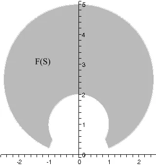
not invariant under a M¨obius transformation ofS2∞: consider, for example, the fractional linear

transformation given by

F :z_{7→ −}1 z.

[image:16.595.352.512.510.681.2]

See Figure 1.1: F maps the starlike domainS to the non-starlike domainF(S).

(17)

There is of course one very natural approach to the problem: consider a sequence of

boundary curves Γi ∈H3 converging to the given curve at infinity, solve the Plateau problem

for H-surfaces for each Γi, and then extract a limit out of the solution surfaces. Indeed, in

Chapter 2 we shall successfully employ this approach to prove the following:

Theorem A. Let H∈(−1,1) and suppose Γi ⊂H3 _{is a sequence of Jordan curves converging} to Γ_⊂S∞2 . Suppose ui:B→H3 is a sequence of conformal H-harmonic maps such that ui|∂B

is a parametrisation of Γi. Then, a subsequence converges uniformly on compact subsets of B to a conformal H-harmonic map u:B_→H3 _{such that} _∂

∞(u(B)) = Γ.

As a build up to this result, we now turn our attention to the Plateau problem for H -surfaces on the interior of a (strictly) negatively curved manifold, and identify the role played

by Yau’s isoperimetric inequality.

Our approach to constructing H-surfaces makes use of the fact that such objects have a variational characterisation: they arise as critical points for the functional IH(·) := A(·)−

2HV(_·), where A denotes the area of the surface and V the “enclosed” oriented volume. If the surfaces under consideration have boundary, we enclose a volume by adjoining a reference

surface. We assume for the duration of this section that (N, h) is a complete, simply connected Riemannian 3-manifold of strict negative curvature, and denote by B_{the unit disk in}R2 _with

Cartesian coordinatesz= (x, y). We identify an “origin” o_∈N. In this setting it is convenient to use as reference surface the geodesic cone over the boundary curve, formed by joining every

point on the curve to o via the connecting geodesic. The volume of the resulting domain can be readily calculated. Letu:B_→_N _{be given, and define a map} _F _:B_×_[0_,_1]_→_N _by

F(z, λ)_7→exp_o(λ_·exp−_o1_◦u(z)).

Then F(B_×_[0_,_{1]) defines an oriented 3-chain, which call the geodesic cone over} _u₍B_{), and its}

volume is given by

V(u) =

Z

B×[0,1]

F∗(dV),

(18)

In the hope of applying the direct method we investigate whetherIH satisfies the crucial

properties such as boundedness from below, coercivity and lower semi-continuity. If we restrict

ourselves momentarily to bounded domains with smooth boundary, then in the setting of

man-ifolds with negative curvature the basic result is Yau’s isoperimetric inequality, which we now

state. We also give the simple proof of this result, as it will serve to motivate some of the later

discussion.

Theorem 1.3 (Yau, [52]). Assume N is complete, simply connected and with all sectional curvatures bounded above by -1. Then for any domain ΩinN with compact closure and smooth boundary we have

A(∂Ω)−2V(Ω)>0.

Proof. The result comes from integrating the well known estimate for the Laplacian of the

distance function r(x) :=d(o, x):

∆r>2 cothr >2.

Letν denote the unit outward normal to ∂Ω. Using the divergence theorem we obtain

A(∂Ω)>

Z

∂Ω

(_∇r, ν)dA=

Z

Ω

∆r dV >2V(Ω).

Thus for all such domains, and forH _∈[₋1,1],

A(∂Ω)₋2_|H_|V(Ω)>0.

We shall attempt to promote the notion that the above result not only motivates the

study of H-surfaces in negatively curved manifolds, but also lies at the heart of any existence result. Furthermore, minimisers for the functional Area₋2_×V olume(i.e. H= 1) play a spe-cial role in H3_{, in that they are the borderline case, and we would expect some kind of rigidity}

result - such as the aforementioned result of da Silveira [13]. In particular, the minimal (H = 0) surfaces here do not distinguish themselves - the area functional by itself in hyperbolic space

allows for an abundance of minimisers. Thus we see another, admittedly more heuristic, aspect

(19)

space (the rigorous correspondence is of course given by Lawson’s result [27] that every minimal

surface in Euclidean 3-space is (canonically) locally isometric to a 1-surface in H3_{). Finally, we}

remark that the role of isoperimetric inequalities in existence proofs for H-surfaces has been highlighted before in the literature. We mention in particular the excellent survey article by

Steffen [41].

Analytically the Plateau problem forH-surfaces is formulated as follows: given a Jordan curve Γ_⊂N and a real numberH, find a map u:B_→_N _{such that}

(i) τ(u) + 2Hux∧uy = 0

(ii) (ux, ux)−(uy, uy) = (ux, uy) = 0

(iii) u maps∂B _{homeomorphically onto Γ.}

Here (_·,_·) and_∧denote respectively the inner product and cross product with respect to the ambient metric h, andτ(u) denotes the tension field ofu. Conditions (i) and (ii) together ensure that u(B_{) is an} _H_{-surface. The solution of Plateau’s problem for} _H_{-surfaces in a}

Rie-mannian manifold with an upper bound (not necessarily negative) on the sectional curvatures

was obtained independently by Gulliver [22] and Hildebrandt & Kaul [23] in 1972.

We now revisit the proof of the result of Gulliver and Hildebrandt & Kaul in the setting

of a negatively curved manifold, and show how all the necessary estimates follow from a suitable

integration of the Laplacian of the distance function. Let e(u) denote the energy density of u, given by

e(u) := 1 2 |ux|

2₊_|_u

y|2

,

where, for a tangent vector X,|X|2 _{= (}_{X, X}_{), and denote by}

D(u) :=

Z

B

e(u)dxdy

the Dirichlet energy of u. We use the well established method of working with the Dirichlet functional rather than the area functional,

A(u) :=

Z

B

q

(20)

since the latter is invariant under any reparametrisation whereas D(_·) is only invariant under conformal reparametrisations. We recall that A(u) 6D(u) for all admissable u, with equality if, and only if, u is conformal. Finally define

EH(u) :=D(u)−2HV(u).

Theorem 1.4 ([22],[23]). Let N be a complete, simply connected Riemannian 3-manifold with sectional curvatures all bounded above by -1. Let Γ be a curve satisfying the property that the

space of maps {v : B _→ _N_|_v _maps _∂B _{continuously and monotonically onto} _Γ _and _D₍_v₎ _is finite_} is non-empty. Then for all H _∈[₋1,1] there exists a map u_∈C2₍_B₎_∩_C₍_B₎ _satisfying

(i),(ii),(iii) above.

Sketch proof. We assume we have normal coordinates centred around o. We shall prove a pointwise estimate at a point p0 =u(z0), wherez0 ∈B. Let r0 =|u(z0)|=d(o, p0). We begin

by writingV(u) as an integral overB_:

V(u) =

Z

B

ω(u)dxdy,

where

ω(u)(z0) := Z 1

0

λ2J(λr0)dλ u(z0)·ux(z0)×uy(z0),

and · and × denote respectively the inner and cross product with respect to the Euclidean

metric. J(λr0) denotes the Riemannian density in normal coordinates, evaluated at F(z0, λ).

By definition of∧we can write

ω(u)(z0) = Z 1

0

λ2J(λr0) J(r0)

dλ(u(z0), ux(z0)∧uy(z0)).

Now set

A(r0) := Z 1

0

λ2J(λr0) J(r0)

dλ >0,

so that

|ω(u)_|(z0) =A(r0)|(u(z0), ux(z0)∧uy(z0))|6A(r0)·r0·e(u)(z0),

and by the estimate on the Laplacian of the distance function,

2A(r0)< Z 1

0

∆r(F(z0, λ))λ2

J(λr0)

J(r0)

(21)

Now let a denote the Riemannian density in geodesic polar coordinates. Then J and a are related byt2J(t) =a(t), and we can write

Z 1

0

∆r(F(z0, λ))λ2

J(λr0)

J(r0)

dλ=

Z 1

0

∆r(F(z0, λ))

a(λr0)

a(r0)

dλ.

But the Laplacian of the distance function is given by

∆r(F(z0, λ)) =

a′₍_λr 0)

a(λr0)

,

(see, for example, [9], Chapter 6), and therefore

2A(r0) <

1

a(r0) Z 1

0

a′(λr0)dλ

= 1

a(r0) Z r0

0

a′(ρ)dρ

r0

= 1

r0

.

We thus obtain_|ω(u)_|< 1₂e(u)(z0), and for anyH in the range [−1,1], we have

e(u)₋2Hω(u)>0.

The lower semi-continuity of the integral follows via an application of a lemma of Morrey ([39],

Theorem 1.8.2) which reduces the issue to one of convexity of the integrand. It is easy to check

that in our case positivity of the integrand implies the convexity (see [23], Lemma 4). With

these estimates in place the rest of the proof proceeds via standard methods: one first fixes a

parametrisation of the boundary, and minimises EH within the Sobolev space of W1,2 maps

which agree (in a trace sense) with the given parametrisation on the boundary. This yields a

weak solution to theH-harmonic map equation, and one must then resort to regularity theory to deduce that the solution is in fact smooth. The regularity results needed are discussed in

more detail at the start of Chapter 2. Finally one varies the parametrisation of the boundary

to obtain a map which is also conformal, and which therefore defines anH-surface.

It is worth comparing this with the analogous result in Euclidean space: we can of

course attempt to integrate the expression for the Laplacian of the distance function, but this

now reads as 1/r. This in turn forces us to make the following restrictions on the values of

(22)

|H_|61/R. Thus manifolds withsectN 6−1 distinguish themselves in that we can continue to

solve the Plateau problem for H-surfaces as the boundary curve Γ “tends to infinity”, for any

H in the range (₋1,1). This fact provides much of the motivation for attempting to solve the asymptotic Plateau problem by limiting the Gulliver-Hildebrandt-Kaul solution.

The proof of Theorem A involves two main elements: the first is the control of the

conformal factor for a conformal H-harmonic map, which in turn leads to a uniform gradient estimate for such maps; this result holds in any manifold of strictly negative sectional curvature.

The second is the use ofbarrier surfaces to essentially “trap” the sequence ofH-surfaces within a subdomain of H3_{, and here we will be forced to restrict ourselves to the constant sectional}

curvature case. The full construction is carried out in Chapter 2.

1.3 Perturbation Results

In Chapters 3 and 4 we focus our attention on the issue of continuous dependence of the solution

surface on the boundary curve. We continue to work in the parametric setting. Following the

work of Tromba [46] and Tomi & Tromba [44] on the global analysis approach to the Plateau

problem in R3_{, we view the set of} _H_{-surfaces with prescribed ideal boundary as lying inside}

the set of properH-harmonic maps (defined below) which solve a Dirichlet problem at infinity. Thus we treat separately the issues of H-harmonicity and conformality, and begin by obtaining a perturbation result for H-harmonic maps into hyperbolic 3-space which solve a Dirichlet problem at infinity.

Perturbation of H-Harmonic Maps

Let (U2_{, g}_{) and (}_U3_{, h}_{) denote respectively the upper half space models for hyperbolic space in}

2 and 3 dimensions respectively. A C2 map u:U2_→_U3 _{is said to be} _H_-harmonic _if

(23)

where τ(u) denotes the tension field of u and (e1, e2) is an orthonormal frame field on (U2, g).

We study the linearisation of τH(u), given by the Jacobi operatorJH,u:

JH,u:C∞(U2, u∗TU3) → C∞(U2, u∗TU2)

JH,u:φ 7→ ∆φ+ trgR(du, φ)du+ 2H(d∇φ∧du)(e1, e2),

where C∞₍_U2_{, u}∗_T_U3_{) denotes the space of smooth sections of the pullback bundle, ∆ is the}

rough Laplacian on u∗_T_U3_, _d∇ _and

R denote the connection and curvature tensor of (U3_{, h}₎

respectively, and we have

(d∇φ_∧du)(e1, e2) =d∇φ(e1)∧du(e2) +du(e1)∧d∇φ(e2).

Let (s, t), t > 0 denote the usual rectangular coordinates on U2_{. A simple calculation shows}

us that in these coordinates JH,u takes the form of a uniformly degenerate operator, meaning

that it can be written as a system of polynomials in t∂s and t∂t whose coefficients are at

least continuous up to the boundary∂U2_{. Such operators have been often studied in the past,}

and their mapping properties become apparent when one works in the setting of appropriately

weighted function spaces, where the weight is given by t raised to a power that reflects the degeneracy. We define these function spaces rigorously in Chapter 3, but for the time being it

shall suffice to think of the spaceC_δk,αas consisting of sections ofu∗_T_U_{of the form}_tδ_φ_{, where}_φ

is a section with locallyCk,α _{coefficients, equipped with an appropriate norm. The main result}

of Chapter 3 is the following

Theorem B. Suppose u: (U2_{, g}₎_→₍_U3_{, h}₎ _{is a proper} _H_{-harmonic map with nowhere} vanish-ing energy density on ∂U2_{. Then the Jacobi operator associated to} _u_, _J

H,u, extends to be an

isomorphism JH,u:C_δk,α→C_δk−2,α for all k≥2, and for all δ satisfying 0< δ <3.

This in turn leads to the desired perturbation result:

Theorem C.Assume _|H_| <1. Let u : (U2_{, g}₎ _→ ₍U3_{, h}₎ _{be a proper} _H_{-harmonic immersion} that extends to be a Ck,α _{map from} _U2 _to U3_{, for some} _k _≥ ₂ _and ₀ _{< α <} ₁_{. Assume that} the boundary map f0 := u|∂U2 : R → R2 has nowhere vanishing energy density. Then there

(24)

H-harmonic extension of f, uf ∈ Ck,γ(U2,U3), and furthermore the map f 7→ uf is Ck,γ

smooth.

Remark 1.5. The caseH = 0 here corresponds tou being a harmonic map fromH2 _to_H3_{. The}

asymptotic Dirichlet problem for harmonic maps between hyperbolic spaces was studied by Li

& Tam in [31] and [32], though the issue of continuous dependence on the boundary data was

not addressed. In the current work we restrict ourselves to studying the H2 _to _H3 _{case since}

we are ultimately interested in H-surfaces, but our methods extend to deal with perturbations of proper harmonic maps between hyperbolic spaces of any dimension. The details will be

available in a forthcoming publication [12].

The Conformality Operator and Perturbation of Spherical Caps

In Chapter 4 we prove the following result:

Theorem D.Let H ∈ (−1,1). There exists a neighbourhood η in H5(S1,R2₎ _{of the identity} map id:S1 _→ _R2 _{such that for every} _f _{∈ N} _{there exists a conformal,} _H_{-harmonic extension}

uf satisfying uf|S1 =f.

This is achieved by studying the linearisation of the conformality operatork, defined by the action

k:u_7→h(u∗∂z, u∗∂z),

where u is an H-harmonic map, and ∂z = 1₂(∂x−i∂y) is a section of the complexified tangent

bundleTCB=TB⊗C. h(·,·) here is the complex bi-linear extension of the hyperbolic metric on

U_{. Our approach is very much in the spirit of the aforementioned work of Tomi and Tromba: we}

use methods from complex geometry to show directly that the linearisation of kat a spherical cap ΣH is an isomorphism.

The work in Chapters 3 and 4 has some overlap with recent results of Alexakis & Mazzeo

[2]. They prove the following structure theorem for embedded minimal surfaces in hyperbolic

(25)

Theorem 1.6. Let M be a convex, co-compact hyperbolic 3-manifold, and let _Mk(M) be the

space of properly embedded minimal surfaces in M of genus k with asymptotic boundary curve a C3,α _{embedded, closed (but possibly disconnected) curve in} _∂M_{. Let} _E _{denote the space of all}

C3,α closed embedded curves in ∂M. Then Mk(M) and E are both Banach manifolds and the

projection map

Π :_Mk(M)→ E

is Fredholm of index zero.

1.4 Concluding Remarks

Chapter 2

The Asymptotic Plateau Problem

for

H

-Surfaces

In this chapter we prove a compactness result for sequences of solutions to the Plateau problem

for CMC surfaces on the interior of hyperbolic 3-space. As a consequence of this result we

obtain an immersed disk-like solution to the asymptotic problem. We begin by discussing the

regularity of weak solutions to theH-harmonic map equation. Then, in Section 2.2 we derive a uniform gradient estimate for conformal H-harmonic maps of the unit disk. In Section 2.3 we give the barrier surface construction, and conclude in Section 2.4 with the convergence result.

2.1 Regularity Theory

Letu:B_→_N _{be a (smooth) immersion of the unit disk into a Riemannian 3-manifold (}_{N, h}_).

Assume we have coordinates (x1, x2) onB_{, and let}_h_ij _{denote the coefficients of}_h_{in some choice}

of local coordinates onN. Then theH-harmonic map foruin local coordinates takes the form

∆ul= 2H√hhlm(D1u∧D2u)m−ΓljkDαujDαuk, l= 1,2,3. (2.1)

Here DαX =∂X/∂xα, the summation convention is in place, and Greek indices run from 1 to

2, Latin indices from 1 to 3. Also √h = det(hij) and hij = (hij)−1. Assume now that (N, h)

(29)

way of defining the Sobolev spaces Wk,p₍_B_{, N}_{) as subsets of the familiar} _Wk,p₍_B_,_R3_).

We say a mapu_∈W1,2₍_B_{, N}_{) is a}_{weak solution} _{of (2.1) if for any smooth test function}

with compact supportφ, we have

Z

B

DαulDαφldx=

Z

B

n

Γl_jkDαujDαuk−2H

√

hhlm(D1u∧D2u)m

o

φldx. (2.2) It is straightforward to check that the map obtained during the “fixed boundary

parametrisa-tion” minimisation stage described in the proof of Theorem 1.4 satisfies (2.2). The transition

from weak W1,2 solutions to smooth solutions is essentially a three step process: because the right hand side of (2.1) is quadratic in Dw, one must first show H¨older continuity for the first derivatives before one can apply standard elliptic regularity theory and the usual

“bootstrap-ping” argument kicks in. We describe these steps below.

Remark 2.1. In the work of Gulliver and Hildebrandt & Kaul, the essential estimates on EH

(i.e. coercivity and lower semi-continuity) are obtained by working in a bounded region K of the ambient manifold N (in [23] K is referred to as a gauge ball). The minimisation process is thus carried out only amongst those maps whose image lies within K, and the minimiser w

need not, a priori, be a weak solution of (2.1). To surmount this difficulty, one must first show

continuity of w on B_{. This is achieved via Morrey’s celebrated Dirichlet Growth Lemma ([39],}

Theorem 6.2). In the setting of strict negative curvature any sufficiently large ball will work as

a gauge ball, but the point is that in such a setting one does not need the notion of a gauge

ball at all (as we showed in our proof of Theorem 1.4). In particular we minimise amongst

all W1,2 _{maps into} _N_{, and our minimiser is automatically a weak solution to the}_H_-harmonic

map equation. Furthermore, working within a bounded subdomainKintroduces the additional complication of requiring a inclusion principle that guarantees that the minimiser obtained also

lies entirely within K. Once again, in the case of sectN <0, this additional complication does

not arise.

Step 1 One first obtains H¨older continuity of the solution via an application of Morrey’s

(30)

at z.

Theorem 2.2 (Morrey, [39]). Let w _∈ W1, p(BR(z0)), 1 6 p 6 n. Suppose that for all

z_∈BR(z0), and all r∈(0, ρ(z)], where ρ=R− |z−z0|, Z

r

(z)_|Dw_|pdx6Cp

r ρ

n−p+pδ

(2.3)

holds with δ ∈(0,1]. Then w∈C0,δ(Bs(z0)) for alls < R.

It can be readily shown that the weak solution obtained via the minimisation process

described in Theorem 1.4 satisfies the estimate 2.3 above.

Step 2 One then deduces C1,α regularity (α ∈(0,1)) by means of the following result of Tomi [43]:

Theorem 2.3 ([43]). Suppose that w is a continuous, weak solution for the system

∆w=f(z, w, Dw),

where f satisfies _|f(z, w, Dw)_| 6 µ(_|w_|)_|Dw_|2 _{for some monotonically nondecreasing function}

µ. Then w∈C1,δ for allδ ∈(0,1).

Step 3 Having ascertained that our weak solutionuis inC1,δ, we define functions flby setting

fl := 2H√hhlm(D1u∧D2u)m−ΓljkDαujDαuk, l= 1,2,3.

By Tomi’s result,fl_∈C0,α. We now apply standard elliptic regularity theory to the equation ∆ul=fl,

to conclude thatul ∈C2,δ. The bootstrapping argument now kicks in, since we now know that

fl_∈_C1,δ_{, which implies that} _ul_∈_C3,δ_{, and so on.}

2.2 Uniform Gradient Bound

Assume now that sectN 6 −1. We now obtain a uniform gradient bound for conformal H

(31)

Lemma 2.4. Suppose _|H_|<1, and let u:B_→_N _{be a conformal,}_H_{-harmonic map. Then at} any point z∈B _{we have}

|∇u_|2(z)< Cρ<∞,

where Cρ is some constant depending only on ρ=|z|.

Proof. Since u is conformal andH-harmonic, u(B_{) is an} _H_{-surface. By the Gauss equation we}

have that

Ru =Ku+Rh

where Ru and Rh are the sectional curvatures of u(B) and (N, h) respectively, and Ku is the

extrinsic curvature (i. e. product of principal curvatures) of u(B_). _K_u _{and the mean curvature}

H are related by the inequality

Ku 6H2.

Therefore, since _|H_|<1 and_Rh 6−1 we have

Ru 6H2−1<0. (2.4)

We set ǫ:=√1₋H2_{, so that}_R

u 6−ǫ2.

Now, sinceu is conformal we can write

u∗(h) =λ2_|dz_|2, (2.5)

for some positive functionλonB_{, where}_|_dz_|_{denotes the flat metric on}B_{. In fact,} _λ2 ₌ 1 2|∇u|2.

Set f = lnλ. Note that f is bounded on B_{, by definition. By the formulae for a conformal}

change of metric we obtain the differential inequality

∆f ≥ǫ2e2f =:η(f).

We wish comparef with the solution to the differential equation

∆φ=η(φ),

given by

φ(z) = ln 2

(32)

Letψ:=f₋φ. We claim thatψ(z) 60 for _|z_|<1. Indeed, supposeψ >0 at some point. We note thatψ→ −∞ as|z| →1, therefore ψ must take a positive maximum at some pointp∈B

with _|p_|<1. By continuity, ψ >0 on some neighbourhood_N of p. Therefore, on _N, we have ∆(ψ) = ∆(f)−∆(φ)≥η(f)−η(φ) >0. Thus ψis subharmonic on N, contradicting the fact that it had a maximum at p. We conclude that

f(z)6ln 2

ǫ(1_{− |}z_|2₎,

so that λmust satisfy

λ(z)6 2

ǫ(1_{− |}z_|2₎,

and

|∇u_|2(z)6 8

ǫ2₍₁_{− |}_z_|2₎2 =:Cρ.

2.3 Construction of Barriers

At this stage we are forced to restrict ourselves to the case N = H3_{. The reason is that our}

barriers are constructed as surfaces equidistant from a totally geodesic surface - a

construc-tion which simply cannot be carried out in a space of variable curvature. Thus from now on

S∞2 =∂∞H3, the sphere at infinity of hyperbolic 3-space, and we assume that we are working

with the unit ball model. Given Γ, an (oriented) Jordan curved on S2

∞ we consider a sequence

Γi of (oriented) Jordan curves converging to Γ. For eachiwe solve the interior Plateau problem for H-surfaces to obtain a sequence ui(B) of surfaces of constant mean curvature H and with

∂(ui(B)) = Γi. We now show that if the sequence of curves {Γi} converges to Γ within some

special, fixed region ofH3_{, then the corresponding surfaces Σ}i_{also lie entirely within this region.}

Similar constructions have previously been described by Alencar & Rosenberg [1], Tonegawa

[45] and most recently Coskunuzer [11].

We begin by noting that Γ separates S∞2 into two disjoint open disks. We fix and label

these two regions as Ω+ _{and Ω}−_{. The given orientation on Γ combined with some fixed}

(33)

H _∈(₋1,1), we wish to span Γ by a CMC surface whose mean curvature isH with respect to this normal. We now take a circle U contained entirely inside Ω+, and we consider the totally geodesic surface spanning U. U also separates S2

∞ into two regions, and we label the region

contained entirely inside Ω+as Ω+_U. Finally we construct the equidistant surface that has mean curvature_|H_|with respect to the normal that points towards Ω+_U. With our convention (mean curvature = ₋1₂tr A, A = second fundamental form) this surface will be the one lying on the side towards Ω+_U. We call these surfaces|H|-caps. In a similar manner we take a circle in Ω−_,

set Ω−_U to be that part ofS2

∞\U entirely contained in Ω− and take the cap of constant mean

curvature |H|with respect to the normal that points towards Ω−_U. Each |H|-cap separates H3

into two regions. Modifying the terminology of [11] we call these regions_|H_|-shifted half-spaces, and if Γ is contained in one of these half-spaces then we say the half-space issupporting.

Finally we perform this construction for all circles lying inS∞2 \Γ, and make the following

definition:

Definition 2.5. The _|H_|-shifted convex hull of Γ is defined to be the intersection of all sup-porting _|H_|-shifted half-spaces, and is denoted by_CH(Γ).

We claim:

Lemma 2.6. If a sequence of curves {Γi} converging to Γ lies entirely within CH(Γ), then so

too does the sequence of H-surfaces _{ui(B)}, where ∂(ui(B)) = Γi.

We shall use the following maximum principle:

Lemma 2.7. Let Σ1 _and _Σ2 _{be two hypersurfaces in a Riemannian manifold that intersect}

tangentially at a common point p. Let Hi be the mean curvature of Σi at p. If Σ1 lies on the positive side of Σ2 then H1> H2.

By positive side we mean the side opposite to the direction indicated by the chosen

reference normal atp. This is dictated by our convention for the mean curvature.

Remark 2.8. We note that since we are working with immersed surfaces, we cannot refine the

(34)

-after choosing a reference normal ν, say, one cannot know beforehand whether the surface one is trying to control has mean curvature +|H|or −|H|with respect toν.

Proof of Lemma 2.6: Let Γ0be a Jordan curve contained inCH(Γ), and let Σ0be theH-surface

with boundary Γ0_{. We must show that Σ}0 _{does not intersect any non-supporting half-space.}

Let W be a non-supporting half-space, i. e. W _⊂H3 _and _W _∩_{Γ =}_∅_{. Suppose Σ}0 _enters _W_.

We can foliate W by |H|-caps whose asymptotic boundaries lie in S∞2 . Since Γ0∩W =∅, Σ0

must intersect some_|H_|-capK tangentially at some pointp. We choose as reference normal at

p the normal νp that places (according to our convention) Σ0 on the positive side ofK. The

maximum principle then implies that the mean curvature of Σ0 _{must be strictly greater than}

that ofK. Our construction ensures that with respect toνp,K will have mean curvature +|H|,

while Σ0 _{will have mean curvature either +}_|_H_|_or _−|_H_|_{. In either case we obtain a violation of}

the maximum principle.

2.4 Compactness

Theorem A. Let H∈(−1,1) and suppose Γi ⊂H3 _{is a sequence of Jordan curves converging} (in the Hausdorff distance) to Γ _⊂ S2

∞. Suppose ui : B → H3 is a sequence of conformal

H-harmonic maps such that ui|∂B is a parametrisation of Γi. Then, a subsequence converges

uniformly on compact subsets of B _{to a conformal} _H_{-harmonic map} _u _: B _→ H3 _{such that}

∂∞(u(B)) = Γ.

Proof. Let Ω be a compact subdomain of B_{. By the uniform gradient estimate there exists a}

constant C such that

sup

z∈Ω|∇

ui(z)|2hyp < C <∞for all i, (2.6)

whereCdepends only on the domain Ω. Letz0∈Ω. From the barrier argument we may assume

that_|ui(z0)|hyp <∞ for all i, so that by the mean value theorem and (2.6), we obtain

sup

z∈Ω|

ui(z)|< C <∞ for all i, (2.7)

(35)

Next, we again define functionsfl

i on Bby setting

f_il:= 2H√h(ui)hlm(ui)(D1ui∧D2ui)m−Γljk(ui)Dαu_ijDαuki, l= 1,2,3.

We apply Schauder theory to the equation

∆ul_i =f_il

to obtain the estimate

|ul_i_|_C1,α_(Ω′₎6C

sup

Ω |

f_il_|+ sup

Ω |

ul_i_|

, α_∈(0,1),

for some Ω′ _⋐_{Ω. But, by definition,}

|fl

i|is bounded above on compact subsets by a multiple of

|∇ul_i|2_{, which is in turn bounded above by some uniform constant, as described above. Therefore}

we obtain a uniformC1,α _{bound for}_ul

i, which in turn implies a uniformC0,α bound forfil. We

then use the estimate

|ul_i_|_C2,α_(Ω′₎6C

|f_il_|_C0,α_(Ω)+ sup Ω |

ul_i_|

to obtain a uniformC2,αbound onul_i, and so on. Thus for every multi-indexγ, the sequence of partial derivatives _{|Dγui|}is uniformly bounded. We may now apply Ascoli-Arzela’s theorem

to conclude that a subsequence of {ui} converges to a mapumΩ′ inCm(Ω

′_{) for all} _m_{, and finally}

using a diagonal process on an increasing sequence of relatively compact domains inB_{we extract}

a further subsequence converging to a map u in C∞₍_B_{) which is} _H_{-harmonic, conformal and}

satisfies∂∞(u(B)) = Γ.

Remark 2.9. The closest result of this kind in the literature is Anderson’s Theorem 4.1 in [6],

where he proves the existence of complete, embedded, minimal surface of the type of the disk,

asymptotic to a given Jordan curveγ on the sphere at infinity ofH3_{. The initial steps are similar}

to our own: he considers a sequence of C2 Jordan curves on the interior of H3 _{converging to}

γ. Through the work of Almgren & Simon [4] he asserts the existence of a smooth, embedded minimal disk spanning each element of the sequence. By establishing appropriate bounds on the

mass (in the GMT setting) of the intersection of these disks with ever increasing geodesic balls,

(36)

result to conclude that Σ is first a regularly embedded minimal surface, and then that it is of

(37)

Chapter 3

Perturbation of Proper

H

-Harmonic

Maps

The main object of study in this chapter is the linear operatorJ that arises as the linearisation at an H-harmonic map of the H-tension field operator τH. We shall apply the implicit

func-tion theorem on Banach spaces to deduce a perturbafunc-tion result forH-harmonic maps between hyperbolic 2-space and hyperbolic 3-space, and for this we require J to be invertible between appropriate function spaces. J turns out to be a uniformly degenerate elliptic edge operator, and the analysis of its mapping properties requires the use of certain weighted function spaces,

which we define in Section 3.3. A simple indicial root analysis, carried out in Section 3.4, yields

a maximal interval for the weights on which we expect J to be invertible. The invertibility result is proved in Section 3.4.3 using a combination of basicL2 estimates and techniques from Mazzeo’s edge calculus [34].

3.1 The

H

-Harmonic Map Equation and its Linearisation

Ultimately our interest lies in the perturbation of maps from the Euclidean unit disk into

hy-perbolic 3-space. However for the purpose of our analysis, it will suit us to also introduce the

hyperbolic metric on the domain. The H-harmonic map equation (Definition 3.1) is confor-mally invariant, so we are free to do this. Furthermore, the calculations become particularly

(38)

and target. Thus let (U2_{, g}_{) denote the upper-half space in} _R2_{, with coordinates (}_{s, t}_), _{t >} _0,

equipped with the hyperbolic metricg:= ge/t2, where ge denotes the Euclidean metric onU2;

(U3_{, h}_{) will, as usual, denote the 3-dimensional upper-half space model.}

Definition 3.1. LetH _∈R_{. For a}_C2 _map _u_{: (}_U2_{, g}₎_→ ₍_U3_{, h}_{) we define the} _H_{-tension field}

of u, denoted τH(u) by

τH(u) :=τ(u) + 2Hdu(e1)∧du(e2), (3.1)

whereτ(u) denotes the tension field ofu, anddu(e1)∧du(e2) denotes the cross-product ofdu(e1)

and du(e2) with respect to the metrich, where e1 =t∂t,e2 =t∂s. u is said to beH-harmonic

if τH(u) = 0.

We will study perturbations of solutions to the equation τH(u) = 0 by means of the

implicit function theorem. We therefore study the linearisation of theH-tension field operator

τH, linearised at an H-harmonic mapu:

JH,u(φ) = ∇∂t|t=0τH(ut) = ∆φ+ trgR(du, φ)du+ 2H(d ∇_φ

∧du)(e1, e2), (3.2)

where {ut} is a variation of u satisfying ∇∂t|t=0ut = φ, ∆ denotes the rough Laplacian on

the pullback bundleu∗₍_T_U3_),_d∇ _and

R denote respectively the connection and the curvature

tensor of (U3_{, h}_{), and}

d∇φ∧du(e1, e2) =d∇φ(e1)∧du(e2) +du(e1)∧d∇φ(e2).

Definition 3.2. We callJH,u theJacobi operator, and solutions to JH,uφ= 0Jacobi fields.

Remark 3.3. Recall that when H = 0 our basic objects are examples of the familiar harmonic maps between Riemannian manifolds. The Jacobi operator in this case has been the subject of

much study, though primarily for situations with compact domain and target. As an example

of recent work in this direction we mention the work of Lemaire & Wood [29] onintegrable (i.e.

arising as the variation vector field through a 1-parameter family of harmonic maps) Jacobi

(39)

In terms of the local coordinates (s, t), the components of the H-tension field of a map

u= (a, b, c) : (U2_{, g}₎_→₍_U3_{, h}_{) are given by}

τ_H1(u) =t2

¯ ∆a₋2

c∇¯a·∇¯c+

2H

c (bsct−btcs)

(3.3)

τ_H2(u) =t2

¯ ∆b₋2

c∇¯b·∇¯c+

2H

c (csat−ctas)

(3.4)

τ_H3(u) =t2

¯ ∆c+1

c |∇¯a|

2₊_|_∇_¯_b_|2_{− |}_∇_¯_c_|2₊2H

c (asbt−atbs)

(3.5)

where ¯∆, ¯∇, · and | · |e denote respectively the Euclidean Laplacian, gradient, inner product

and norm onU2_.

In our current set-up, the “spherical caps” described in Chapter 1 take the form of

sur-faces equidistant to a totally geodesic copy ofU2 _{inside (}_U3_{, h}_{). Their} _H_-harmonic

parametri-sations are given by

ΣH : (s, t)7→

tH, s, tp1−H2_, _H_∈₍₋₁_,₁₎_, _(3.6)

where, if (x, y, z), z > 0, are coordinates on U3_{, the totally geodesic copy of} _U2 _{in (}_U3_{, h}_{) is}

defined by theyz-plane, and the ΣH have the y-axis as shared ideal boundary.

3.2 Asymptotics of

H

-Harmonic Maps

In this section we analyse a formal series solution to theH-harmonic map equation. This anal-ysis serves two purposes: it will allow us to construct a first approximate solution to τH = 0

(which we later perturb to an exact solution), and will also yield the asymptotic behaviour of

H-harmonic maps. This latter information will be important in understanding the nature of the degeneracy of the linearised operator JH,u.

We assume for the moment thatu: (U2_{, g}₎_→₍_U3_{, h}_{) is a proper}_H_{-harmonic map that}

is smooth onU2_{, and solves a Dirichlet problem at infinity. Let} _u₍_{s, t}_{) = (}_a₍_{s, t}₎_{, b}₍_{s, t}₎_{, c}₍_{s, t}_)).

(40)

as formal power series:

a(s, t) = a0(s) +a1(s)t+a2(s)t2+a3(s)t3+O(t4) +. . .+O(tn)

b(s, t) = b0(s) +b1(s)t+b2(s)t2+b3(s)t3+O(t4) +. . .+O(tn)

c(s, t) = c1(s)t+c2(s)t2+c3(s)t3+O(t4) +. . .+O(tn)

(we know that c(s, t) = 0 when t= 0). Denote now by f0 = (a0, b0) :R→R2 the restriction of

u to the boundary, and bye(f0) the energy density off0, given by

e(f0) = ∂a0 ∂s 2 + ∂b0 ∂s 2 .

From now on we will use ′ to denote differentiation with respect to s. Assume that e(f0) is

nowhere vanishing onR_{, and that}_|_H_|_<_{1. Substitution of the above series expansion into the}

H-harmonic map equation yields a system of ODEs for the coefficient functions ai, bi and ci.

This can be done by hand, but is readily handled by a computer algebra system such as Maple.

For example, the first three equations, arising from equating to 0 the coefficients of the tterm in the series expansion of τH(u), are

−2a1+ 2Hb′0= 0

−2b1−2Ha′0= 0

1

c1

a2₁+b2₁+e(f0)−c21−2H(a1b′0−a′0b1) = 0

The resulting system of ODEs can easily be solved either by hand or again using software. It

turns out that a1, b1, c1, a2, b2 and c2 are all formally determined by a0 andb0. The coefficients

for the cubic termt3are formally undetermined by the equation, and all higher order coefficients depend ona0, b0, a3, b3 andc3. More precisely we have the following asymptotics for properH

-harmonic maps whose boundary maps have nowhere vanishing energy density:

a1=Hb′0, b1=−Ha′0, c1 = p

e(f0)(1−H2) (3.7)

a2 = ₂_e₍1_f0) a

′′

0(b′0)2{1−2H2}+ 2a′0b′0b′′0{H2−1} −(a′o)2a′′0

(3.8)

b2 = ₂_e₍1_f0) b

′′

0(a′0)2{1−2H2}+ 2b′0a′0a′′0{H2−1} −(b′o)2b′′0

(3.9)

c2= q

1−H2

e(f0)(a

′

(41)

In particular we note that ∂u ∂t · ∂u ∂s t=0

=a1a′0+b1b′0 = 0

∂u ∂t · ∂u ∂t t=0

= (a1)2+ (b1)2+ (c1)2 =e(f0)

∂u ∂s · ∂u ∂s t=0

= (a0)2+ (b0)2 =e(f0)

where · denotes the Euclidean inner product. Thus such maps are automatically “Euclidean

conformal” at the boundary (cf. Section 1.4).

We can actually derive the first order asymptotics for an H-harmonic map u assuming thatu extends to be merelyC1 onU2_{, and without resorting to a power series analysis. In the}

caseH= 0 this result was obtained by Li & Tam [31]. We will need the following simple lemma from [31]:

Lemma 3.4([31], Lemma 1.2). Letp be aC1 _{function on}_U2 _{that is smooth on}U_{. Let}_t_denote the Euclidean distance to the boundary∂U2_{. Then for any point}_x_∈_∂_U2 _{there exists a sequence}

{xi} ⊂U2 with xi →x such that

lim

i→∞t(xi) ¯∆p(xi) = 0.

We now prove:

Lemma 3.5. Let H _∈ (₋1,1). Suppose u = (a, b, c) : (U2_{, g}₎ _→ ₍_U3_{, h}₎ _{is a proper} _H -harmonic map that extends to be a C1 map from U2 _to U3_{. Assume that the boundary map}

f0 :=u|∂U2 :R→R2 has nowhere vanishing energy densitye(f₀). Thenusatisfies the following

first order compatibility conditions:

∂a ∂t t=0

=H ∂b ∂s t=0 , ∂b ∂t t=0

=₋H ∂a ∂s t=0 , ∂c ∂t t=0

=pe(f0)(1−H2).

Proof. From (3.5) we have that

t2∆¯c+t

2

c |∇¯a|

2₊_|_∇_¯_b_|2_{− |}_∇_¯_c_|2₌ 2Ht2

c ∂a ∂t ∂b ∂s − ∂a ∂s ∂b ∂t . (3.11)

We multiply (3.11) by c/t2 _{to obtain} _c

t

t∆¯c+ |∇¯a|2+|∇¯b|2− |∇¯c|2= 2H

(42)

Now let x _∈ R_{, and let} _{_x_i_} _{be the sequence of points in} B _{converging to} _x _{constructed in}

Lemma 3.4. Evaluating (3.12) at xi and lettingi→ ∞we obtain that at t= 0

∂a ∂t 2 + ∂b ∂t 2 + ∂a ∂s 2 + ∂b ∂s 2 − ∂c ∂t 2

= 2H

∂a ∂t ∂b ∂s − ∂a ∂s ∂b ∂t . Now, ∂a ∂t ∂b ∂s 6 1 2 ∂a ∂t 2 +1 2 ∂b ∂s 2 ,

and similarly for ∂a_∂s∂b_∂t. Therefore

∂c ∂t 2 = ∂a ∂t 2 + ∂b ∂t 2

+e(f0)−2H ∂a ∂t ∂b ∂s − ∂a ∂s ∂b ∂t (3.13) > ∂a ∂t 2 + ∂b ∂t 2

+e(f0)−H ( ∂a ∂t 2 + ∂b ∂t 2)

−He(f0) (3.14)

= (1₋H)

( ∂a ∂t 2 + ∂b ∂t 2)

+ (1₋H)e(f0) (3.15)

>0.

Therefore ∂c ∂t t=0 6

= 0. (3.16)

Applying the same idea to the equation τ1

H(u) = 0, we obtain, at t= 0,

∂a ∂t

∂c ∂t =H

∂b ∂s

∂c

∂t, (3.17)

and since ∂c_∂t ₆= 0, we conclude that

∂a ∂t t=0

=H ∂b ∂s t=0 . (3.18)

Similarly, fromτ2

H(u) = 0, we obtain

∂b ∂t t=0

=₋H ∂a ∂s t=0 . (3.19)

Finally, substituting (3.18) and (3.19) into (3.13) we obtain

∂c ∂t t=0

(43)

In particular we have that for such a mapu= (a, b, c),

lim

t→0

t c =

1

p

e(f0)(1−H2)

<_∞ (3.20)

In fact, we have the following important corollary of Lemma 3.5, entirely analogous to

Corollary 1.4 in [31]:

Corollary 3.6. Assume H ∈ (−1,1). Let u be an H-harmonic map from (U2_{, g}₎ _to ₍_U3_{, h}₎ that extends to be a C1 _{map from} _U2 _to U3_{. Suppose that} _f

0 := u|∂U2 has nowhere vanishing

energy density as map from R _toR2_{. Then the hyperbolic energy density} _e₍_u₎ _{is bounded, and} furthermore

lim

t→0e(u) =

2

1₋H2. (3.21)

We now use the asymptotics (3.7)-(3.10) to extend an arbitrary boundary map to a map

of U2 _whose_H_{-tension field vanishes to second order.}

The Extension Operator _E

Assume we have anH-harmonic mapu: (U2_{, g}₎_→₍_U3_{, h}_{) which extends to be at least}_C2_{up to}

the boundary, and assume, as always, that the boundary mapf0=u|U2 :R→R2 has nowhere vanishing energy density e(f0). Let f = (f1, f2) be some given map again satisfying e(f) 6= 0

everywhere onR_{, that lies in a}_C2,α₍_R_,_R2_{) neighbourhood of}_f

0. We begin by extendingf to a

map ˜f = ( ˜f1_,_f˜2_,_f˜3_{) :}_U2 _→_U3_{, where the ˜}_fi _{are polynomials in}_t_{of order 2 whose coefficients}

are functions of f1(s) and f2(s) determined by the asymptotics (3.7)-(3.10). In the same way we extendf0 to ˜f0. Note that these extensions areC2 only on a neighbourhood of t= 0. Next

we pick a smooth cut-off functionχ which equals 1 on a small enough neighbourhood oft= 0, and define

E(f) :=χ( ˜f₋f˜0) +u. (3.22)

For a section φ of the pullback bundle u∗_T_U3_{, let} _|_φ_|

e denote the Euclidean norm of φ. The

operator E has been specifically concocted to ensure that it extends an arbitrary boundary

Complete noncompact CMC surfaces in hyperbolic 3 space

University of Warwick institutional repository: http://go.warwick.ac.uk/wrap

A Thesis Submitted for the Degree of PhD at the University of Warwick

http://go.warwick.ac.uk/wrap/3135

This thesis is made available online and is protected by original copyright.

Please scroll down to view the document itself.

Complete Noncompact CMC Surfaces

in Hyperbolic 3-Space

Thomas Cuschieri

Mathematics Institute

Contents

Acknowledgments

Declarations

Abstract

Chapter Breakdowns and

Preliminaries

Chapter Breakdowns

Preliminaries

Chapter 1

CMC Immersions and the

Isoperimetric Inequality

1.1

The Basic Models

1.2

The Plateau Problem for

H

-Surfaces and the Isoperimetric

Inequality

1.3

Perturbation Results

1.4

Concluding Remarks

Chapter 2

The Asymptotic Plateau Problem

for

H

-Surfaces

2.1

Regularity Theory

2.2

Uniform Gradient Bound

2.3

Construction of Barriers

2.4

Compactness

Chapter 3

Perturbation of Proper

H

-Harmonic

Maps

3.1

The

H

-Harmonic Map Equation and its Linearisation

3.2

Asymptotics of

H

-Harmonic Maps