WORKING PAPERS SERIES
WP06-19
The Markov-Switching Multifractal Model of
Asset Returns: GMM Estimation and Linear
Forecasting of Volatility
The Markov-Switching Multifractal Model of
Asset Returns: GMM Estimation and Linear
Forecasting of Volatility
April 5, 2006
Abstract
Multifractal processes have recently been proposed as a new formalism for modelling the time series of returns in finance. The major attraction of these processes is their ability to generate various degrees of long memory in different powers of returns - a feature that has been found in virtually all financial data. Initial difficulties stemming from non-stationarity and the combinatorial nature of the original model have been overcome by the introduction of an iterative Markov-switching multifractal model in Calvet and Fisher (2001) which allows for estimation of its parameters via maximum likelihood and Bayesian forecasting of volatility. However, applicability of MLE is restricted to cases with a discrete distribution of volatility components. From a practical point of view, ML also be-comes computationally unfeasible for large numbers of components even if they are drawn from a discrete distribution. Here we propose an alter-native GMM estimator together with linear forecasts which in principle is applicable for any continuous distribution with any number of volatility components. Monte Carlo studies show that GMM performs reasonably well for the popular Binomial and Lognormal models and that the loss incurred with linear compared to optimal forecasts is small. Extending the number of volatility components beyond what is feasible with MLE leads to gains in forecasting accuracy for some time series.
Keyword: Markov-switching, multifractal, forecasting, volatility, GMM estimation
JEL Classification: C20, G12
1
Introduction
The recent proposal of multifractal models (Calvet et al., 1997; Calvet and Fisher, 2001, 2002a) has added an interesting new entry to the rich variety of volatility models available in financial econometrics (cf. Poon and Granger, 2003, for an up-to-date review). The essential new feature of this class of models is its multiplicative, hierarchical structure of volatility components with hetero-geneous frequencies. Research on multifractal models originated from statistical physics where they had been proposed as models for turbulent flows (e.g. Man-delbrot, 1974). The main attraction in the financial sphere is the ability of these models to generate different degrees of long-term dependence in various powers of returns - a feature pervasively found in all financial data (cf. Ding, Engle and Granger, 1993; Andersen and Bollerslev, 1997; Lobato and Savin, 1999). Unfortunately, multifractal models used in physics were of a combina-torial rather than causal nature and they suffered from non-stationarity due to the limitation to a bounded interval and the non-convergence of moments in the continuous-time limit. These major weaknesses were overcome by Calvet and Fisher (2001) who introduced a Markov-switching multifractal model based on Poisson arrival times for which weak convergence to the continuous-time limit could be demonstrated. The interpretation as a Markov-switching process (al-beit with a possibly huge number of states) also allowed maximum likelihood estimation of the parameters for cases with a discrete distribution of volatility components and forecasting based on the current conditional probabilities of volatility states. The implementation of this procedure in Calvet and Fisher (2004) showed that this new model provides gains in forecasting accuracy for medium and long horizons (up to 50 days) over forecasts from GARCH and FIGARCH models.
Our contribution to this emergent literature in this paper is twofold: (i) we introduce an alternative GMM estimator of multifractal parameters which could be used in cases in which ML is not applicable or computationally infeasible, (ii) we propose linear forecasting which also is universally applicable and does not require particular specifications of the distribution or restrictions on the number of volatility components. We first explore the behavior of GMM plus linear forecasting against the benchmark of ML and optimal forecasts for the special case of the Binomial model used in Calvet and Fisher (2004). As it turns out, GMM is, of course, less efficient than ML but it is nicely behaved in that it has small biases and reasonable mean squared errors for the crucial multifractal parameters. Monte Carlo results are in good harmony withT12 consistency and
no problems of non-convergence or multiplicity of solutions are encountered in our simulations. Furthermore, despite the sometimes sizable difference in Monte Carlo MSEs between GMM and MLE, differences are less pronounced with respect to forecasting performance: GMM with linear forecasts typically only has a very slight disadvantage against ML-based optimal forecasts. Additional Monte Carlo runs also show that the performance of GMM and linear forecasts is not adversely affected by increasing the number of volatility components or by replacing the discrete Binomial distribution of multipliers by a continuous Lognormal distribution.
optimal predictors. Section 5 presents our empirical findings before we provide concluding remarks in section 6. Two appendices provide detailed derivations of the moment conditions used for GMM estimation, and closed-form solutions of autocovariances needed to construct best linear forecasts.
2
The Markov-Switching Multifractal Model
Multifractal measures have a long history in physics dating back at least to the early seventies when Mandelbrot introduced them as models for the distri-bution of energy in turbulent dissipation (e.g., Mandelbrot, 1974). The main reason for considering multifractal processes in the financial context is that they share certain properties which are known to be universal characteristics of asset returns as well: they have hyperbolically decaying autocovariances (long mem-ory) and fat tails. Multifractality, furthermore, implies that different powers of the measure have different decay rates of their autocovariances. While early empirical evidence of multifractality in financial data had already appeared in, e.g., Vassilicos et al. (1993), Calvet et al. (1997) were the first to develop a multifractal model for financial data. TheirMultifractal Model of Asset Returns (MMAR) assumes that returns follow a compound process in which an incre-mental Brownian motion is subordinate to the cumulative distribution function of a multifractal measure. Calvet and Fisher (2002a) develop estimators and diagnostic tests for this model on the base of its scaling properties.
However, despite the attractiveness of its stochastic properties, practical applicability of the MMAR suffered from its combinatorial nature and its non-stationarity due to the restriction to a bounded interval. These limitations have been overcome by the iterative time series models introduced by Calvet and Fisher (2001, 2004). Calvet and Fisher (2001) define a continuous-time multifractal model with random times for the changes of multipliers (Poisson multifractal) and demonstrate weak convergence of a discretized version of this process to its continuous-time limit. This approach preserves the hierarchy of volatility components of MMAR but dispenses with its restriction to a bounded interval. In the discretized version of the Poisson multifractal, the volatility dy-namics can be interpreted as a Markov-switching process with a large number of states. As long as the state space from which volatility components are drawn is finite maximum likelihood can be used for parameter estimation and Bayesian probability updating allows forecasting of future volatility. Forecasting algo-rithms developed for this model have been successfully applied for forecasting exchange rate volatility in Calvet and Fisher (2004).
In the following, we shortly review the building blocks of this Markov-Switching Multifractal process (MSM). Returns are modelled as:
xt=σt·ut (1)
with innovationsutdrawn from a standard Normal distribution N(0,1) and instantaneous volatility being determined by the product ofkvolatility
compo-nents or multipliersMt(1),M
(2)
t ...,M
(k)
t and a constant scale factorσ:
σ2t =σ2 k !
i=1
Mt(i). (2)
Each volatility component is renewed at timetwith probabilityγidepending on its rank within the hierarchy of multipliers and remains unchanged with probability 1−γi. The transition probabilities are specified by Calvet and Fisher (2001) as:
with parametersγk∈[0,1] andb∈(1,∞). Estimation of this model, then,
involves the parametersγkandbas well as those characterizing the distribution
of the components Mt(i). In the present paper, we explore two specifications for the distribution of multipliers: the Binomial and Lognormal MSM mod-els. Following Calvet and Fisher (2004) the Binomial MSM is characterized by Binomial random draws taking the values m0 and 2−m0 (1 ≤ m0 < 2)
with equal probability (thus, guaranteeing an expectation of unity for allMt(i)). The model, then, is a Markov switching process with 2k states whose parame-ters can be estimated via maximum likelihood. Conditional state probabilities can be used to compute forecasts of future volatility and these are shown to outperform forecasts derived from GARCH, FIGARCH, and two-state Markov switching GARCH models. While this approach is optimal for the Binomial MSM as well as multinomial generalizations, its general applicability is limited in two respects: First, it is not applicable for models with an infinite state space, i.e. continuous distributions of the multipliers. Second, current computational limitations make choices ofk beyond 10 unfeasible even for the Binomial case
because of the implied evaluation of a 2k
×2ktransition matrix in each iteration.1
In the following we consider both specifications with a continuous distribu-tion of multipliers and large numbers of multipliers, k > 10. As an example
of a multifractal model with a continuous state space we consider the Lognor-mal MSM model with volatility components drawn from a Lognormal distri-bution (cf. Calvet and Fisher (2002a) for the earlier non-stationary Lognormal MMAR). In this model, multipliers are determined by random draws from a Lognormal distribution with parametersλands, i.e.
Mt(i)∼LN(−λ, s2). (4)
Normalisation viaE[Mt(i)] = 1 leads to
exp(−λ+ 0.5s2) = 1, (5)
from which a restriction on the shape parameter can be inferred: s=√2λ.
Hence, the distribution of volatility components is parameterized by a one-parameter family of Lognormals with the normalization restricting the choice of the shape parameter.
Given the successful performance of the Binomial MSM withk ≤10 inves-tigated in Calvet and Fisher (2004), it appears certainly worthwhile to explore whether one would get similar or better results by increasing the number of volatility components or adopting a continuous distribution of the multipliers. To this end, we introduce a GMM estimator as a flexible and versatile estimation method for multifractal parameters and compare its performance to that of ML (where applicable), and we complement GMM estimation by linear forecasting on the base of estimated parameter values which can be used as a substitute for Calvet and Fisher’s Bayesian forecasts if conditional state probabilities are not available. Both approaches are applicable to a wide variety of specifications of (1) and (2). In order to concentrate on the estimation of the parameters of the distribution of volatility components and to confine the overall number of parameters to be estimated via GMM, we restrict the specification of transition probabilities by fixingex antetheir parameters,bandγk, and focusing on
esti-mation of the parameters of the distribution of volatility components. Following the recommendation of an anonymous referee, we imposed the restrictionsb= 2
and γk = 0.5. Note that the later restriction implies that the volatility
com-ponent at the highest frequency has a probability of one-half to be replaced
1For multinomial specifications with more than two states, computational limitations would
by a new draw. We have performed a limited sensitivity analysis by replacing this second parameter byγk= 0.99 which would amount to replacement of the
component at the high-frequency end with a probability close to 1 (reminiscent of the earlier MMAR model in which the high-frequency component is replaced with certainty in every period).2 We found a certain trade-offbetween the
re-striction on γk and results for estimated distributional parameters (reported below), but little overall difference in goodness-of-fit of the MSM model and its forecasting performance.3
3
Estimation of Markov-Switching Multifractal
Models via GMM
Estimation of multifractal models has proceeded from adaption of the so-called “scaling estimator” in Calvet et al. (1997) for the combinatorial MMAR – which is still pervasively used in natural sciences – to the seminal proposal of maximum likelihood estimation for the discretized MSM in Calvet and Fisher (2004). MLE is optimal in those cases in which it can be applied and has the added advantage of providing conditional probabilities of the unobserved volatility states which can be exploited for optimal forecasts on the base of the transition matrix of the model.
However, because of the restriction of MLE to discrete distributions of multi-pliers and computationally feasible values ofk, it appears worthwhile to explore
alternative ways of estimating MSM parameters. To this end, we follow some earlier attempts at investigating method of moments estimation. However, in contrast to the SMM (Simulated Method of Moments) approach in Calvet and Fisher (2002b), we use a GMM (Generalized Method of Moments, cf. Hansen, 1982) approach with analytically solvable moment conditions. We shortly re-view the basic GMM framework before turning to our particular set of moment conditions. In GMM, the vector of parameter estimates of a model, sayϕ, is obtained as:
"
ϕT = arg min ϕ∈ΦfT(ϕ)
"A
TfT(ϕ) (6)
withΦthe parameter space,fT(ϕ) the vector of differences between sample moments and analytical moments, andAT a positive definite and possibly ran-dom weighting matrix. As is well-known, ˆϕT is consistent and asymptotically Normal if suitable ‘regularity conditions’ are fulfilled (sets of which are detailed, for example, in Harris and M´aty´as, 1999). ˆϕT then converges to
T1/2( ˆϕT −ϕ0)∼N(0,Ξ) (7)
with covariance matrixΞ= ( ¯FT"V¯T−1F¯T)−1in whichϕ0is the true parameter vector, ˆVT−1=T varfT( ˆϕT) is the covariance matrix of the moment conditions,
ˆ
FT(ϕ) = ∂f∂ϕT(ϕ) is the matrix of first derivatives of the moment conditions, and ¯
VT and ¯FT are the constant limiting matrices to which ˆVT and ˆFT converge. Applicability of GMM would have been cumbersome for the MMAR ap-proach of Calvet et al. (1997) and Calvet and Fisher (2002a) because of its
2Note that one could also assume additional stages of the cascade at non-observable
fre-quencies beyond the one at which data are available. Any assumption on the number of unobservable submerged components could be used to compute their expected contribution to the marginal distribution at the frequency of available data.
3We have also tried the simpler specificationγi= 2−(k−i), also without much of an effect
non-stationarity violating the required regularity conditions. This problem, for-tunately, does not carry over to the MSM model which rather fits into the class of Markov-switching models with standard asymptotic behavior. As has been pointed out by Calvet and Fisher (2004), although models of this class are par-tially motivated by empirical findings of long-term dependence of volatility, they donot obey the traditional definition of long-memory, i.e. asymptotic power-law behavior of autocovariance functions in the limitt → ∞ or divergence of the spectral density at zero (cf. Beran, 1994). MSMs are rather characterized by only ‘apparent’ long-memory with an asymptotic hyperbolic decline of the auto-correlation of absolute powers over a finite horizon and exponential decline thereafter. In the case of Markov-Switching multifractal processes, therefore,
Cov(|xqt|,|xqt+τ|)∝τ2d(q)−1 (8)
holds only over an interval 1 * τ * bk with b the number of states (i.e.
b= 2 in the binomial MSM) and kthe number of multipliers.
Although applicability of regularity conditions is not hampered by this type of “long memory on a bounded interval”, the proximity to ‘true’ long memory might rise practical concerns. For example, note that withb = 2 and k= 15,
the extent of the power law scaling might exceed the size of most available data for daily financial prices. In finite samples, application of GMM to Markov-Switching multifractals could, then, yield poor results since usual estimates of the covariance matrixVT might show large pre-asymptotic variation.
Our practical solution to this potential problem is using log differences of absolute returns together with the pertinent analytical moment conditions, i.e. to transform the observed dataxt into:
ξt,T = ln|xt|−ln|xt−T|. (9)
As is shown in Appendix A, the transformed variableξt,T, in fact, only has non-zero auto-covariances over a limited number of lags. With non-overlapping observations, we only observe non-zero auto-covariances at lag one, i.e. forξt,T andξt+T,T, while for overlapping log differencesξt,T,ξt+1,T, ...auto-covariances would be non-zero over T lags. In our applications below, overlapping obser-vations are used. One may note that moments ofξt,T only depend on the pa-rameters of the volatility process while the standard deviation of the Normally distributed increments,σ, drops out when computing log differences:
ξt,T = ln # # # #σut(
k $
i=1
Mt(i))
1 2
# # # #−ln
# # # #σut−T(
k $
i=1
Mt(−i)T)12
# # # #
= 0.5
k %
i=1
(ε(i)
t −ε
(i)
t−T) + ln|ut|−ln|ut−T| withε(ti)= ln(M
(i)
t ).
The lack of inclusion of the scale parameter σ in the above parameter set makes it necessary to add another moment condition such as the second moment ofxtthat exactly identifiesσ.
In order to exploit the temporal scaling properties of the multifractal model, our GMM estimator uses moment conditions providing information over various time horizons. In particular, we select covariances of the powers of ξt,T, i.e. moments of the following type:
forq= 1,2 andT = 1,5,10,20 together with E(x2
t
) =
σ2 for identification of
σ. Since the eight moment conditions for m0 or λ are not affected by σ, the
covariance matrix of the parameters should be block-diagonal and estimated values ofσshould be essentially identical to the sample standard deviation.
Note that our moment conditions differ from those used in previous litera-ture. Calvet and Fisher (2002b) had used a variety of moment-scaling properties, parameters of log-log regressions of the sample auto-covariogram, slope parame-ters from log-periodogram regressions, high-frequency auto-covariances and tail index estimates. They report that the covariogram and tail index estimates showed the lowest mean squared errors. Earlier versions of this paper had also applied high-frequency auto-covariances following the example of the stochastic volatility literature (Andersen and Sørensen, 1996). However, experimentation indicated that the performance of these moment conditions was quite sensitive to the underlying parameter values of the multifractal model. In contrast, as will be shown in our Monte Carlo simulations below, using log-moments leads to relatively homogeneous behavior across the parameter valuesm0andλand even
more so across different choices of k. This nice behavior of log-moments might
be attributed to the resulting linear connection of (log) volatility components instead of their multiplicative relationship in the raw data.
An alternative Simulated Method of Moments (SMM) approach has been pursued recently by Calvet, Fisher and Thompson (2006) for estimation of the parameters of a bi-variate MSM model. They use a particle filter to optimize the simulated likelihood of the bivariate Binomial model within a two-step es-timation approach that can be interpreted as a SMM estimator. In comparison to this approach, our GMM estimator is based on analytical moments which considerably reduces computational demands.
It might be worthwhile to also try various combinations of our moment conditions for log increments and other moments used in previous research which might provide additional scope for increasing the efficiency of GMM. However, a comprehensive investigation into potential gains from various sets of alternative moment conditions is beyond the scope of the present paper and might be left for future research.
We proceed by reporting results of several Monte Carlo studies designed to explore the performance of our new GMM estimator. Due to the moderate com-putational demands of GMM, we were able to use an iterative GMM scheme in which a new weighting matrix is computed and the whole estimation process is repeated until convergence of both the parameter estimates and the weighting matrix is obtained (cf. Hansen, Heaton and Yaron, 1996). Variance-covariance matrices of moment conditions and, hence, the weighting matrices of the subse-quent iteration are computed numerically. Inspection of the variance-covariance matrices shows that both in our Monte Carlo simulations and in the empirical application, the block-diagonal structure is apparent as the covariance between the estimators ofmo orλandσis close to zero.
We start with the Binomial Model with a limited number of multipliers,
k= 8, and subsequently increase the number of volatility components and also
switch to the Lognormal model as an example of a specification with continuous state space.4 Our first experiments serve to establish the efficiency of the GMM
4Earlier versions of this paper also included comparisons with the traditional “scaling
estimates vis-`a-vis the ML approach of Calvet and Fisher (2004) for a setting
that is close to the Monte Carlo experiments reported in their paper. To this end, we choose multipliers m0 = 1.3, 1.4 and 1.5 and sample sizesT1 = 2500,
T2= 5000, andT3= 10000. The only difference of our simulation set-up is that
we fixed the parameters of the transition probabilities (3) asb= 2 andγk= 0.5
so that we only have to estimate two parameters compared to four in Calvet and Fisher’s somewhat more general approach. Results are displayed in Table 1. Comparison with the pertinent table in Calvet and Fisher (2004) shows that in the more parsimonious two-parameter model bothm0 andσ can be estimated
somewhat more efficiently than with four parameters. Furthermore, Table 1 indicates that biases and root mean squared errors of the ML estimates ofm0
are hardly affected at all by the choice of parameters, while RMSEs appear to increase for σ for higher m0. This is plausible since with increasing m0
one generates enhanced fluctuations of the product of volatilities which might interfere with the estimation of the constant scale factor.
Table 1 about here
Comparison of MLE and GMM estimates shows, of course, that the later are less efficient.5 Obviously, variability of estimates form
0with GMM is much
higher, ranging from 4 to 10 times that of the ML estimates. The relative difference is the higher, the smaller the sample size and the lower the ‘true’ value m0. While biases and MSEs of ML estimates of m0 were essentially
independent of the true parameter, GMM estimates exhibit a decrease of both the bias and MSEs when proceeding from m0 = 1.3 to m0 = 1.5. A closer
look reveals that the larger bias for smallermo is caused by a certain number of cases in which the estimator gets locked-in at the lower boundary (mo = 1) of the admissible parameter space. The farther the true parameter is above the boundary the fewer are these cases so that formo = 1.4 or 1.5 practically all estimates are located in the interior of the admissible parameter space and the GMM estimators become essentially as unbiased as ML. In contrast, the quality of the estimates of the scale parameterσis almost identical under both methods with only a very slight advantage for ML against GMM. Interestingly, the average bias of the Monte Carlo estimates is moderate throughout and quickly approaches zero for the larger sample sizes.6 It is also worthwhile to
point out that the GMM estimator is quite well-behaved in that we encounter no problems of non-convergence or breakdown of the estimation in all our Monte Carlo simulations. This is in contrast to GMM estimation of standard stochastic volatility models which are plagued by a non-negligible frequency of ‘crashes’, cf. Andersen and Sørensen (1996).
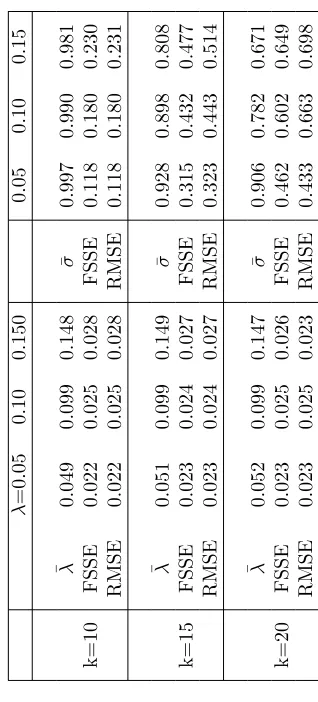
Now, we proceed into territory in which MLE becomes unpractical, at least for the purpose of simulation studies. Table 2 shows GMM results for the same set of parameters but with an increasing number of cascade components,
subsequent development of ML techniques. Experiments with varying numbers of moments in our GMM approach indicated monotonic behavior with a steady reduction of simulated mean squared errors when increasing the number of moments. Because of decreasing returns in the gains in precision, using nine moment conditions appeared to yield a satisfactory balance between computational speed and the quality of the estimates. One might, however, keep in mind that the efficiency of GMM could still be increased at reasonable computational costs.
5However, one might note that obtaining our GMM estimates with nine moment conditions
requires only a small fraction of the time needed for ML estimation.
6In view of our concerns about the proximity of the MSM with its ‘long memory on a
bounded interval’ to processes with pure long-term dependence, it is also interesting to note that our estimates are in harmony withT12 consistency (with a slightly slower convergence rate in the casem0= 1.3 due to the influence of boundary solutions). This underscores that
k= 10, 15 and 20. Here we restrict ourselves to only one sample size,T = 5000,
in order to conserve space. Comparison with the pertinent entries in Table 1 shows that the efficiency of multifractal parameter estimates is practically insensitive with respect to the number of components. Inspection of our moment conditions detailed in Appendix A reveals that this is probably so because high-level multipliers are expected to change only very infrequently and, therefore, would only contribute small increments to log differences. On the other hand, these nearly constant entries should make estimation of the scale factorσmore cumbersome as it would be hard to distinguish between long-lived high-level multipliers and an entirely constant factor. This ambiguity is clearly reflected in the blow-up of the FSSEs and RMSEs forσwith increasingk. However, the
almost complete insensitivity of the estimates ofm0with respect to the number
of components might be viewed as a very welcome feature as it implies that estimation ofm0 is hardly affected by potential misspecification ofk.7
Table 2 about here
In the next step, we consider the Lognormal MSM, for which MLE is not applicable at all because of its continuous state space of volatility components. Moment conditions for this model are spelled out in Appendix B. Note that the admissible parameter space for the location parameterλisλ∈[0,∞) where in the borderline caseλ= 0 the volatility process collapses to a constant (the same ifm0= 1 in the Binomial model). Simulations indicate that increasingλleads
to increasing heterogeneity in volatility with 0<λ< 0.2 giving roughly
real-istic appearances of the resulting time series. In our Monte Carlo simulations reported in Table 3 we cover this interval by considering λ = 0.05, 0.10 and
0.15. Again, we only use one sample size,T = 5,000 and numbers of multipliers k equal to 10, 15 and 20. As can be seen, results are not too different from
those obtained with the Binomial model. Biases are negligible for all parameter values of our Monte Carlo study. Interestingly, the danger of lock-in of estima-tors for λ at the lower boundary λ = 0 seems to be non-existent so that the performance of GMM is almost the same for the whole range of ourλs. Again results for λ are also almost insensitive with respect to k, but RMSEs for σ increase monotonically withk. All in all, the picture from both the Binomial
and Lognormal Monte Carlo runs shows that GMM seems to work as well in the continuous case as with a discrete distribution of volatility components.
Table 3 about here
4
Best Linear vs. Optimal Forecasts
ML estimation comes along with identification of conditional probabilities of the current states of the volatility components. Together with the transition matrix of the model, these conditional probabilities can be uses to compute one-step and multi-step forecasts according to Bayes’ rule. Since ML is restricted to discrete distributions, this elegant and optimal way of generating forecasts for multifractal volatility is also restricted to the multi-nomial cases with a finite state space. Again, it would be useful to have methods at hand for specifications beyond the confines of multi-nomial models. One alternative for cases in which MLE is not applicable is to use best linear forecasts. Since these do not require state probabilities as an input, they could also be computed on the base of
7Note also that form
0 = 1.3 biases are even smaller fork≥10 than fork= 8 due to a
GMM parameter estimates. The standard approach for construction of linear forecasts is outlined, for example, in Brockwell and Davis (1991, c.5). Assuming that the data of interest follow a stationary process{Xt} with mean zero, the best linearh-step forecasts are obtained as
"
Xn+h=
n *
i=1
φ(nih)Xn+1−i=φ(nh)Xn, (11)
with the vectors of weightsφ (nh) = (φ(nh1),φn(h2), ...,φ(nnh))" being any solution ofΓnφ(nh) =γ (nh) and γ n(h) = (γ(h),γ(h+ 1), ...,γ(n+h−1))" denoting the auto-covariances for the data-generating process of Xt at lags h and beyond, and Γn = [γ(i−j)]i,j=1,...,n the pertinent variance-covariance matrix. It is well-known, that this approach produces the best linear estimators under the criterion of minimization of mean squared errors. It is also well known, that for long-memory processes, one should use as much information as available, i.e. the vector Xn should contain all past realizations of the process. One might argue that for the MSM, its “long memory on a bounded interval” would lead to an optimal choice of a number of 2k past observations (as auto-covariances would rapidly drop to zero thereafter). However, in our application we simply use all available data as with a ‘true’ long-memory process although very long lags might have no practical influence on the resulting forecasts. The computa-tional demands of these predictors is immensely reduced by using the general-ized Levinson-Durbin algorithm developed recently by Brockwell and Dahlhaus (2004, in particular their algorithm 6).
What is needed to implement linear forecasts is analytical solutions for the auto-covariances of the quantity one wishes to predict. In our case, our aim is to predict squared returns,x2
t, as a proxy of volatility which requires analytical solutions forE[x2
t+nx2t]. These are also given for the Binomial and Lognormal models in Appendices A and B, respectively. Implementing (11), we have to consider the zero-mean time series:
Xt=x2t−E[x2t] =x2t−"σ2 (12)
whereσ"is the estimate of the scale factorσin eq. (2).8
Again, our aim is to first explore how much is lost by using linear instead of optimal forecasts and, then, to investigate the performance of linear forecasts in cases in which optimal forecasting is infeasible or unpractical.
Our first example parallels the comparison of MLE and GMM for the Bi-nomial model withk = 8 in Table 1. To conserve space, we restrict ourselves
to one sample sizeT = 10,000 using half of the data for in-sample parameter
estimation and the remainder for assessment of the out-of-sample forecasting performance in terms of mean-squared error (MSE) and mean absolute error (MAE). Including MAEs seems interesting since the best linear estimators are those among all linear forecasts which minimize mean squared errors. It, there-fore, appears worthwhile to also explore their performance with respect to a different criterion. Both MSE and MAE are standardized relative to the MSE and MAE of the most naive forecast, i.e. the sample standard deviation or ‘historical volatility’ during the in-sample period, for the same sample, so that values below 1 indicate an improvement against the constant variance forecast by the pertinent model. Three different forecasting procedures are shown in Table 4: “ML” uses Bayesian updating together with ML parameter estimates
8Note that!σonly appears in the mean value of eq. (12), but it drops from the coefficients
as detailed in Calvet and Fisher (2004), “BL1” uses best linear forecasts on the base of GMM parameter estimates, and “BL2” uses best linear forecasts together with ML parameter estimates. The later variant has been added to see how much of a potential loss of efficiency might be due to the use of linear forecasts vs. Bayesian updating and how much to GMM vs. ML. However, as it turned out, we never observe much of a loss of efficiency anyway from using either BL1 or BL2.
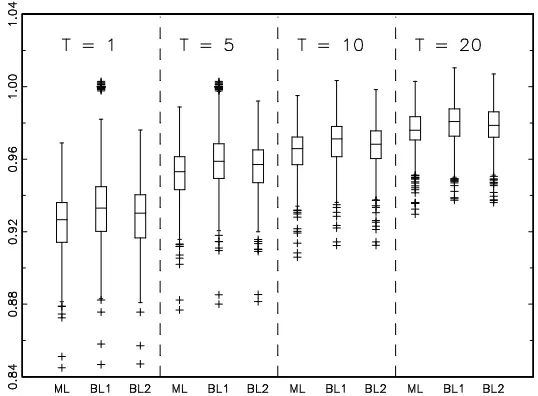
As can be seen from the average MSEs and MAEs in Table 4, as expected, ML mostly comes out as the most efficient method but its advantage against BL1 and BL2 is tiny, with the later on average reaching about 99 percent of the efficiency of ML for most parameters and forecasting horizons. We also illustrate the full distribution of Monte Carlo MSEs for one case (m0 = 1.3)
in Fig. 1. As can be seen from the box-plots, the entire distribution of MSEs seems to be quite similar for our three different approaches. The only slight difference between the three methods is that BL1 produces a number of outliers with standardized MSE equal to one. These corresponds to those cases with parameters estimatesm+0 = 1 for which multifractality vanishes and predicted
volatility is identical to historical volatility. However, the overall performance (in terms of mean and median predictive performance) is hardly affected by these cases and the boundary estimates do hardly occur any more for higher values of m0. Although linear forecasts are geared towards minimization of MSE,
the difference between ML based Bayesian forecasting and linear forecasting are practically the same with the MAE criterion. On the other hand, it also appears worth mentioning that ML seems to come along with a somewhat higher variability than BL1 and BL2 under MAE comparison so that one would have to compare higher average gain with higher dispersion of forecasting quality when choosing between these three methods. Table 4 also indicates that forecast quality depends on the multifractal parameterm0: increasing m0 from 1.3 to
1.4, we observe decreasing MSEs and particularly MAEs. This might be a consequence of the more pronounced volatility clustering with higherm0. Note,
however, that this trend continues for MAEs when proceeding to m0 = 1.5,
while MSEs rather deteriorate slightly at long time horizons.
Table 4 and Figure 1 about here
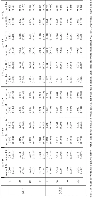
In parallel with our investigation of GMM estimation in sec. 3, we now extend the scope of our Monte Carlo analysis to cases that can not (or only at prohibitive computational cost) be dealed with on the base of ML based meth-ods. To this end, Table 5 shows results for the Binomial model with numbers of volatility componentsk= 10, 15 and 20 and similar experiments for the
contin-uous parameter case of the Lognormal MSM. In both cases, we only have one method available, GMM estimation together with linear forecasts (the former BL1).
The basic message of Table 5 is that with a higher number of volatility components, squared returns have a larger predictable component. For example, for one-day horizons andm0= 1.3, the predictable component (the decrease of
our relative MSEs) increases from 6.5 percent at k = 8 to 15.1 percent with k = 20. For the twenty day horizon we observe an increase from 2.0 percent
(k = 8) which probably is irrelevant in an applied context to 10.4 percent
(k = 20) which might be more interesting. We have also included long time
horizons of fifty and one hundred lags which still have improvements of about 8 to 9 percent compared to the MSE of the sample variance. Results are fairly homogeneous across multifractal parameters as well as for both the MSE and MAE criterion, but forecastability seems to be higher for higher values ofm0.
period constant at T = 5000 in all these experiments. This means that the
information used to estimate the parameters has not been increased with k.
One might also note that the increase in biases and estimation variability of the constant componentσ with increasing k (cf. Tables 2 and 3) does not appear
to be a major obstacle to successful prediction of future volatility.
Pretty similar results are obtained with the Lognormal specification. Gains in predictability are about the same as with the Binomial model for increasing numbers of volatility components. Investigating a larger set of parameter values (available upon request), we found that the variation of MSE and MAE for the Lognormal model is often non-monotonic under variation ofλ. In particular, we observe a rather pronounced U shape in MSEs with forecastability improving forλ= 0.10 againstλ= 0.05 but decreasing again for λ= 0.15. We conjecture
that this variability is due to the lower degree of homogeneity in the volatility clustering of the Lognormal process in which multipliers are drawn randomly from an infinite support. Higher λ also leads to a higher dispersion of the Lognormal variates via s = √2λ so that the volatility of volatility increases,
which might explain the deterioration of forecastability for higherλ.
Table 5 about here
5
Empirical Evidence
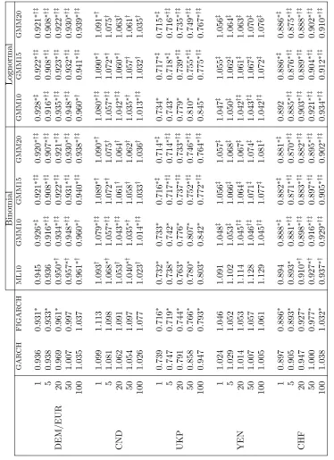
We now turn to empirical data in order to see whether using GMM plus linear forecasting helps improve on previous ML estimates together with optimal fore-casts. Potential gains could result from the accessability of richer specifications, i.e. allowing for additional multipliers beyond the constraints of about k≤10 and from using distributions with continuous rather than discrete state space for the multipliers.
Our empirical analysis uses data from five different foreign exchange markets: The Deutsche Mark exchange rate against the U.S.$ extended by the EURO from 1999 (DEM/EUR) and the exchange rates of the British Pound (UKP), the Canadian Dollar (CND), Japanese Yen (YEN) and Swiss Franc (CHF), all against the U.S. Dollar. All time series start on 1 January 1979 and extend until 31 December 2004. All data were obtained from Datastream. Most series consist of buying rates computed at noon in New York (YEN, UKP, CND), while the DEM/EURO - U.S. Dollar exchange rates are based on snapshots of USD quotes from multi-contribution sources taken at 4 p.m. London time, and the Swiss Franc exchange rate is the one compiled by the Swiss National Bank at 11 a.m. GMT. Investigation of these foreign exchange rates is interesting as these time series (with the exception of CHF) have also been used in the recent study by Calvet and Fisher (2004) who found improvements of the MSM model over GARCH type models in out-of-sample forecasts of volatility. We have also studied the performance of our GMM approach for some other financial data (the stock market indices DAX of the German stock market, the New York Stock Exchange Composite Index, and the price of gold) and report on pertinent results below (details are available upon request).
pertinent GARCH and FIGARCH results. Except for the Canadian Dollar, the MSM model is preferred over the alternative models by these statistics, which nicely confirms results reported in Calvet and Fisher (2004).
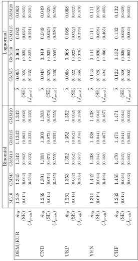
Table 6 reports in-sample parameter estimates for the multifractal param-eters m0 or λ from both the Binomial and Lognormal specification. For the
sake of brevity we skip the second parameterσin eq. (1) as there is less gen-uine interest in this scale factor. For the Binomial model, results based on ML estimation withk = 10 as well as GMM withk= 5,10,15 and 20 are shown,
whereas the lack of applicability of ML estimation only leaves us with the later choice in the case of the Lognormal model.
Inspecting the results, a number of observations are remarkable9: in
particu-lar, for the GMM approach, parameter estimates form0andλare practically the
same with different numbers of multipliers for both the Binomial and Lognormal model. In fact, if one monitors the development of estimated parametersm0
andλwith increasingk, one finds strong variation initially with a pronounced
decrease of the estimates at small numbers for k which becomes slower and
slower until, eventually, a lock-in at a constant value can be found somewhere betweenk= 10 andk= 15. As can be seen from Table 6 estimates still undergo
slight variations when proceeding fromk= 5 to 10 but they remain practically
unchanged thereafter. It is not too difficult to see why this happens: inspection of moment conditions in the Appendix (e.g. eq. (A7) and (A8) for the Bino-mial model, and (B3) and (B4) for the Lognormal model) shows that additional high-level multipliers make a smaller and smaller contribution to the moments so that their numerical values would stay almost constant. This small influence of additional elements in the hierarchy of multipliers also suggests that it should be hard or impossible to distinguish between multifractal models with different numbers of components oncek increases beyond a certain threshold.
While GMM parameter estimates are very homogeneous over different spec-ifications ofk, the ML and GMM parameter estimates show no particular
co-herence across time series. Table 6 also shows the probability of Hansen’s test statisticsJT=fT( ˆϕ)"AˆTfT( ˆϕ), which apparently does not change at all beyond
k = 10. This observation also suggests that the similarity of models with a
different number of volatility components with respect to their moments ham-pers model selection on the base of the objective function. We tried model comparisons along the line of the SMM approach in Calvet and Fisher (2002b) combining the minimized moment functions with simulated weighting matrices for varying numbersk", but results were practically constant across all choices
ofk and k" beyond some threshold. It is plausible that the lack of sensitivity
of moments onkbeyond a certain value would carry over to the weighting
ma-trices as well so that the discriminatory power of such comparisons should be extremely limited. We would expect a similar pattern to apply to likelihood ratio tests for comparison of highkand k" even if the truek is the larger one if these tests were computationally feasible.10 Model selection among
compet-ing specifications of multifractal models with different numbers of multipliers, therefore, remains a challenging task. In view of the inconclusive results, we choose to take an agnostic approach and to investigate the performance of
var-9For the alternative setting with fixed parametersb = 2 and γk = 0.99 the
multifrac-tal parameters (m0 and λ) were typically slightly below those reported here, while overall
goodness-of-fit and forecasting capacity were almost the same. It appears plausible that a higher frequency of replacement at the high-frequency end leads to more volatility and, there-fore, gives rise to a compensatory reduction of the heterogeneity of the multipliers.
10Calvet and Fisher (2004) report results of a likelihood ratio test of models with 10
compo-nents against models withk= 1 to 9 multipliers. Though they find monotonically increasing
ious specifications in predicting future volatility.
Table 7 about here
As another remarkable finding in Table 6, the similarity of the probability of theJ statistic (and therefore, also the optimized value of this statistic) for
the Binomial and Lognormal model stands out. The numbers are, in fact, prac-tically identical for both time series under all specifications of the number of volatility components. This shows that both the Binomial and Lognormal can fit our selection of moments equally well. Therefore, allowing for a continu-ous distribution of multipliers seems not to improve upon the performance of the discrete case with two states only, where 2k possible combinations, for suffi -ciently highk, seem to provide enough flexibility for capturing the heterogenous
volatility dynamics. Note also that estimated MSM models can fit our selection of moments quite well: except for the case of the Swiss Franc theJ-test
statis-tics would not allow to reject the MSM as the data-generating process on the base of our chosen moment function.
Parsimony of model design might suggest to restrict oneself to a relatively small number of multipliers, given the inconclusive results of specification tests for high values k. Note, however, that increasing k does not come along
with additional parameters. On the other hand, higher k implies a larger
re-gion of apparent long memory. In empirical data, hyperbolic decline of the auto-correlations of absolute and squared returns is observed over many or-ders of magnitude without any apparent cut-offand significantly positive auto-correlations have been found at extremely long lags. For the daily S&P 500 returns, Ding, Granger and Engle (1993) found significant auto-correlations at over 2700 lags, i.e. about 10 years. Since higherk implies a longer power-law
range of the autocorrelations, the longer dependence in volatility might improve forecasting performance. As has been shown in section 3, with the same num-ber of in-sample observations, mean squared errors and absolute errors decline at all forecasting horizons for increasing k while the quality of the estimates
of the multifractal parametersm0andλremains essentially unchanged. These
findings provide the perspective that higher choices of k could also improve
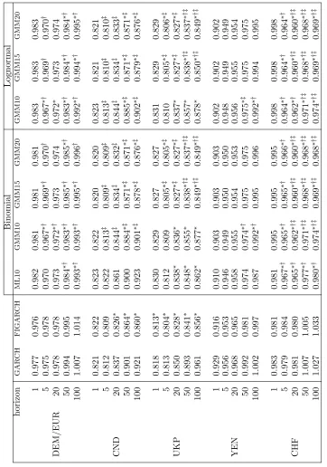
volatility forecasts for empirical data. Tables 7 and 8 explore this issue for our selection of foreign exchange rates. For all five time series we compare forecasts over horizons varying from one day over 5, 20, 50 to 100 days. The models we use are: GARCH and FIGARCH as benchmarks from the traditional time series literature, the Binomial MSM withk= 10 estimated by ML as well as the
Binomial and Lognormal MSM with k= 10, 15 and 20 estimated by GMM.11
MSEs and MAEs are again reported relative to those of historical volatility. Results are not entirely homogenous, but are quite encouraging. First, in-specting out-of-sample MSE (cf. Table 7), we see that in all cases but one some or all versions of MSM do outperform GARCH and FIGARCH. The one excep-tion is the Canadian Dollar where FIGARCH has a slight advantage over MSM at most time horizons (which is in nice conformity with the in-sample domi-nance of the FIGARCH model for this series). Multistage forecasts typically exhibit an increasing advantage of MSM against GARCH/FIGARCH at longer
11Estimated GARCH and FIGARCH models can be found in Appendix C. Despite certain
prediction horizons. The Diebold-Mariano test for differences in predictive ac-curacy allows to reject GARCH in favor of MSM in the Canadian Dollar and both, GARCH and FIGARCH in favor of MSM for the Deutsche Mark/EURO, British Pound and Swiss Franc at long horizons. For the Japanese Yen, the MSM’s relative mean squared errors are the lowest over all time horizons, but differences are not significant at the 5 percent confidence level. For the MAE criterion (cf. Table 8) results are very similar. We find an overall dominance of MSM against (FI)GARCH in four time series: Deutsche Mark/EURO, Cana-dian Dollar, British Pound and Swiss Franc. The one outlier here is the Japanese Yen, for which the baseline GARCH model has the lowest MAE. Note, however, that the best predictor for both the Canadian Dollar and Japanese Yen exchange rate volatility under MAE is the historical average and all time series models lead to a deterioration against this naive prediction (i.e. MAEs are larger than one) in the two cases.
So far our results essentially confirm the findings reported in Calvet and Fisher (2004). Now turn to a detailed assessment of the new linear forecasts based on GMM parameter estimates for Binomial models with k > 10 and
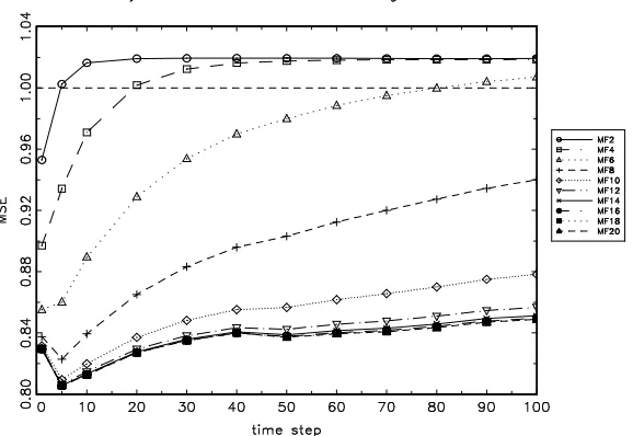
Lognormal models with their continuous distribution of multipliers. The first question on which we would let our data speak is whether a higher number of components improves forecasting performance. Considering the development of MSEs and MAEs with increasing numbers of multipliers in Table 7 and 8, we find that the quality of forecasts improves in the majority of cases. Significant differences between ML and GMM based forecasts are found at the 5 percent confidence level for the Canadian Dollar, British Pound and Swiss Franc under the MSE criterion and for all time series except the Canadian Dollar under the MAE criterion. The effect of the number of multipliers on forecast quality is underscored by Fig. 2 which depicts MSEs for the British Pound/U.S.Dollar exchange rate obtained with linear forecasts on the base of ten multifractal models with k ranging from 2 to 20. As can be seen, increasing k yields a
monotonic improvement which saturates at aboutk≈15. The same behavior
can be found for other exchange rates. Note that we would normally not expect GMM10 to dominate the optimal forecasts from ML10 because of the higher sampling variability of GMM estimates and the suboptimality of linear forecasts. Under this perspective, a somewhat inferior behavior of GMM10 against ML10 would not be surprising. However, in some cases, even atk= 10 GMM estimates
dominate those from maximum likelihood, while for other series increasing k
appears to amount to an overcompensation of the ‘natural’ disadvantage of GMM versus ML.
Tables 7 and 8 about here
Turning to our second objective, it seems worthwhile to remark that the Lognormal model has practically the same performance as the Binomial for each choice ofk at all time horizons so that the added flexibility of the continuous
distribution does not seem to provide an advantage over the simpler discrete structure. This practically identical performance out-of-sample is in harmony with their identical goodness-of-fit in-sample under theJ statistic.
We have also investigated other asset prices along the above lines. For two stock market indices (the German DAX and the New York Stock Exchange Composite Index) and the price of gold we also estimated multifractal parame-ters and investigated their forecasting performance for the same in-sample and out-sample horizons. The in-sample fit of the multifractal model with k= 10
estimated via ML again outperformed the GARCH and FIGARCH models. In contrast, however, theJ test based on GMM parameters estimates rather
moment conditions for all three series. Nevertheless, the comparison of forcast-ing performance turned again out rather favorable for MSM: Under the MSE criterion, we found the estimated MSM models to dominate over GARCH and FIGARCH albeit with fewer significant cases (at the 5 percent level) than with exchange rates. For the DAX and the price of gold, GMM with higher numbers of multipliers also improved upon ML10 forecasts. For the NYSE index, in con-trast, Bayesian forecasts were slightly better than GMM based ones. They also dominated GARCH and FIGARCH forecasts but were not significant at the 5 percent level. The picture was less positive under the MAE criterion, however: for both stock markets, all time series models performed worse than historical volatilities, while in the case of gold, FIGARCH dominated over all other mod-els under the MAE criterion. These somewhat more mixed results certainly call for a more comprehensive analysis of the performance of multifractal models in different types of financial markets.
Before concluding this section, it appears worthwhile to point out another remarkable feature in Table 7 and 8: In quite a number of cases, we see a U-shaped development of MSEs and MAEs at the lower end of our forecast horizons, i.e. the performance increases when moving from the one-period hori-zon to multi-step forecasts over five days and deteriorates thereafter. While one could argue that such behaviour could be due to the lack of parameters modulating short-run dependencies in the MSM framework, the observation of a similar behaviour with FIGARCH in some cases (e.g. Canad. Dollar and UK Pound) casts doubts on such an explanation. Theoretically, all of our candidate models would, of course, lead to a monotonic decline of the quality of forecasts with forecasting horizon as shown in the Monte Carlo simulations in sec. 5 for MSM. While we do not have a ready explanation for this phenomenon at hand, it seems worthwhile to explore in future research whether this is a pervasive feature of financial data or whether it is a particularity of our data sets and the choice of out-of-sample time horizon.
Fig. 2 about here
6
Conclusion
percentage deviation being much smaller than that of mean squared errors of estimated parameters). Extending the state space beyond what is practical with ML (and probably simulated ML as well) could, in principle, lead to higher fore-casting accuracy through the increase of the predictable component of volatility with a higher number of multipliers.
Our empirical application shows, that at least for the majority of foreign ex-change rates investigated, this promise indeed materializes itself. While better performance of MF vis-`a-vis (FI)GARCH had already been demonstrated by
Calvet and Fisher (2004), we show that specifications with a larger state space could provide further improvements in forecasting accuracy. In contrast, re-placing the simple discrete Binomial model by the continuous Lognormal MSM had practically no effect at all: both goodness-of-fit as well as forecasting ca-pability were almost exactly the same for both models. The confirmation of the previous positive results and the further improvements by some alternative specifications documented in this paper underline that multiplicative volatility models with a hierarchy of components should be a promising area of further empirical research.
7
Acknowledgement
References
Andersen, T.G. and T. Bollerslev (1997) Heterogeneous Information Arrivals and Return Volatility Dynamics: Uncovering the Long Run in High Frequency Data,Journal of Finance,52, 975-1005.
Andersen, T.G. and B.E. Sφrensen (1996) GMM Estimation of a Stochastic Volatility Model: A Monte Carlo Study, Journal of Business and Economics Statistics,14, 328-352.
Baillie, R.T., T. Bollerslev and H.O. Mikkelsen (1996) Fractionally Integrated Generalized Autoregressive Conditional Heteroskedasticity, Journal of Econo-metrics,74, 3-30.
Beran, J. (1994) Statistics for Long-Memory Processes. New York: Chapman & Hall.
Brockwell, P.J. and R. Dahlhaus (2004) Generalized Levinson-Durbin and Burg Algorithms,Journal of Econometrics,118, 129-149.
Brockwell, P.J. and R.A. Davis (1991)Time Series: Theory and Methods. New York, Springer.
Calvet, L. and A. Fisher (2001) Forecasting Multifractal Volatility,Journal of Econometrics, 105, 27-58, working paper version: NYU Stern Working Paper FIN-99-017 (1999).
Calvet, L. and A. Fisher (2002a) Multifractality in Asset Returns: Theory and Evidence,Review of Economics&Statistics,84, 381-406.
Calvet, L. and A. Fisher (2002b)Regime Switching and the Estimation of Mul-tifractal Processes, Mimeo: Harvard University.
Calvet, L. and A. Fisher (2004) Regime Switching and the Estimation of Mul-tifractal Processes,Journal of Financial Econometrics,2,49-83.
Calvet, L., A. Fisher and B.Mandelbrot (1997) Cowles Foundation Discussion Papers no. 1164-1166, Yale University, available at http://www.ssrn.com.
Calvet, L., A. Fisher and S. Thompson (2006) Volatility Comovement: A Multi-Frequency Approach,Journal of Econometrics,131, 179-215.
Chung, C.-F. (2002) Estimating the Fractionally Integrated GARCH Model. Mimeo: Academia Sinica.
Diebold, F. and R. Mariano (1995) Comparing Predictive Accurancy, Journal of Business and Economics Statistics,13, 253-263.
Hansen, L.P (1982) Large Sample Properties of Generalized Method of Moments Estimators,Econometrica, 50, 1029-1054.
Hansen, L.P., J. Heaton and A. Yaron (1996) Finite-Sample Properties of Some Alternative GMM Estimators,Journal of Business&Economics Statistics,14, 262-280.
Harris, D. and L. M´aty´as (1999) Introduction to the Generalized Method of Mo-ments Estimation, Chap. 1 in: L. M´aty´as, ed.,Generalized Method of Moments Estimation, Cambridge: University Press.
Lobato, I.N. and N.E. Savin (1998) Real and Spurious Long-Memory Properties of Stock Market Data,Journal of Business&Economics Statistics,16, 261-283.
Mandelbrot, B. (1974) Intermittent Turbulence in Self Similar Cascades: Diver-gence of High Moments and Dimension of Carrier,Journal of Fluid Mechanics,
62, 331-358.
Poon, S.-H. and C. Granger (2003) Forecasting Volatility in Financial Markets: A Review,Journal of Economic Literature,41, 468-539.
Vassilicos, J.C., A. Demos and F. Tata (1993) No Evidence of Chaos But Some Evidence of Multifractals in the Foreign Exchange and the Stock Market, in: Crilly, A.J., R.A Earnshaw and H. Jones, eds., Applications of Fractals and Chaos. Berlin: Springer.
Vilasuso, J. (2002) Forecasting Exchange Rate Volatility, Economics Letters,
76, 59-64.
Appendix
A
Moments of Binomial Model
In order to apply GMM and to compare its performance with that of the ML approach, we have to compute closed-form solutions for selected moments of the Binomial model. As pointed out in the main text, we use a selection of moments of log increments together with the second moment of the raw data. In order to apply GMM, we have to derive analytical solutions for this set of moment conditions. Let
µt=
k !
i=1
Mt(i) (A1)
denote the volatility process andηt,T its log increments:
ηt,T = ln(µt)−ln(µt−T) = k *
i=1
ln(Mt(i))− k *
i=1
ln(Mt(−i)T). (A2)
It is readily apparent thatE[ηt,T] = 0 for all T. Let us now consider the first
auto-covariance ofηt,1:
E[ηt+1,1ηt,1] =E
. k
*
i=1
/
ε(ti+1) −ε(ti)
01
k *
j=1
/ ε(tj)−ε
(j)
t−1
0
(A3)
withε(ti)= ln /
Mt(i)
0 .
Because of independence of any pair of volatility componentsiand j, only
summands withi=jgive non-zero contributions to the term on the right-hand
side. Furthermore, it can easily be seen that these components, i.e.
E&/ε(ti+1) −ε (i)
t 0 /
ε(ti)−ε
(i)
t−1
0'
are themselves different from zero only if the relevant multiplier changes two times betweent−1 andt+ 1.
In general,
E&/ε(ti+1) −ε (i)
t 0 /
ε(ti)−ε
(i)
t−1
0' =
E&ε(t+1i) ε(ti) '
−E8/ε(ti) 029
−E&ε(ti+1) εt(−i)1'+E&ε(ti)ε
(i)
t−1
'
.
(A4)
Since in order to get non-zero entries, we have to have: ε(ti+1) =ε (i)
t−1 ,=ε
(i)
t and
this happens with probability (1 2γi)
2, the above expression becomes:
:1
2γi ;2
<
2 ln(m0) ln(2−m0)−ln2(m0)−ln2(2−m0)=. (A5)
We, therefore, arrive at
E[ηt+1,1ηt+1] = <2 ln (m0) ln (2−m0)−ln2(m0)−ln2(2−m0)=
·
k *
i=1
:1
2γi ;2
In passing, we note that auto-covariances at higher lagsτ>1, i.e.
E[ηt+τ,1ηt,1] =E
>. k *
i=1
/
ε(ti+)τ−ε
(i)
t+τ−1
01 .*k
i=1
/ ε(ti)−ε
(i)
t−1
01?
are all equal to zero because of the independence of changes betweent−1 and
tand betweent+τ−1 andt+τ (τ>1), respectively.
Considering the autocovariances of the log changes over time intervalsT >1,
we have to replace the probabilities for renewal after one time step by the pertinent probabilities for T steps which leads to:
E[ηt+T,Tηt,T] = <2 ln (m0) ln (2−m0)−ln2(m0)−ln2(2−m0)=
·
k *
i=1
1 4
/
1−@1−γiAT02. (A7)
The calculations become slightly more involved when considering the auto-covariances of squared log increments:
E(ηt2+T,Tη2t,T
)=
E
.*k
i=1
/
ε(ti+)T −ε
(i)
t
012
k *
j=1
/ ε(tj)−ε
(j)
t−T
0
2
. (A8)
Again, one can arrive at a relatively simple formula by identifying the non-zero entries and their probabilities of occurrence. Let us start with T = 1.
Three cases are relevant here:
(1) i=j andε(ti+1) ,=ε (i)
t ,=ε
(i)
t−1:
This leads to entries of the form:
(ε(i)
t+1−ε
(i)
t )2(ε
(i)
t −ε
(i)
t−1)2
= (ln (m0)−ln (2−m0))2(ln (2−m0)−ln (m0))2
= ln4(m
0) + ln4(2−m0) + 6 ln2(m0) ln2(2−m0)
−4 ln3(m0) ln (2−m0)−4 ln (m0) ln3(2−m0)≡χ.
Note that the relevant sequences m0 → m1 → m0 or vice versa again
happen with probabilities (1 2γi)2.
(2) i,=j andε(tj+1) ,=ε (j)
t andε
(i)
t ,=ε
(i)
t−1.
It can easily be seen that for non-zero entries, this leads again to /
ε(tj+1) −ε(tj) 02/
ε(ti)−ε
(i)
t−1
02
= (ln (m0)−ln (2−m0))4=χ
which is the same as in (1) and occurs for each pairi,=jwith probabilities
(1 2γi)(
1 2γj).
(3) i,=j andεt(+1n) ,=ε(tn),=ε
(n)
t−1,n=i, j in entries of the form
(εj
t+1−ε
j
t)(εit+1−εit)(ε
j
t−ε
j
which again is identical to (ln(m0)−ln(2−m0))4=χ . The probability
of this to happen is (1 2γi)
2(1 2γj)
2 but we also have to take into account
that each of these terms appears two times in the expansion ofη2
t+1,1ηt,21
in (A8).
Putting cases (i) to (iii) together we arrive at:
E(η2t+1,1η2t,1
)=
k *
i=1
:1
2γi
;*k
j=1
:1
2γj
;
+ 2
k *
i=1
:1
2γi
;2 *k
j=1,j$=i
:1
2γj ;2
χ.
(A9)
For arbitrary T, we get:
E(ηt2+T,Tηt,T2
)=D%k
i=1
.
1 2
/
1−(1−γi)T0%k
j=1
1 2
/
1−(1−γj)T0 1
+2%k
i=1
.
1 4
/
1−(1−γi)T02 %k
j=1,j$=i
1 4
/
1−(1−γj)T02 1E
χ.
(A10)
Turning to the log innovations of the compound process,
ξt,T = ln|xt|−ln|xt−T|, we find:
E[ξt+T,Tξt,T] =E
F: 0.5
k %
i=1
/
ε(ti+)T −ε(ti) 0
+ln|ut+T|−ln|ut| ;
: 0.5
k %
i=1
/ ε(ti)−ε
(i)
t−T
0
+ln|ut|−ln|ut−T| ;G
= 0.25·E[ηt+T,Tηt,T] + (E[ln|ut|])2−E &
(ln|ut|)2 '
,
(A11)
and
E(ξ2
t+T,Tξt,T2
) =
E
.
0.5
k *
i=1
/
ε(ti+)T −ε(ti) 0
+ln|ut+T|−ln|ut| 12
. 0.5
k *
i=1
/ ε(ti)−ε
(i)
t−T
0
+ln|ut|−ln|ut−T| 12
= 0.252·E(η2t+T,Tη2t,T )
−<E(η2t,T )
−E[ηt+T,Tηt,T]=
·N(E[ln|ut|])2−E &
(ln|ut|)2 'O
+ 3·E&(ln|ut|)2 '2
−4·E[ln|ut|]E &
(ln|ut|)3 '
+E&(ln|ut|)4 '
. (A12)
We also note that the expectation of the squared log increment of the volatil-ity process is:
E(η2t+T,T
) =
k *
i=1
1 2
/
1−(1−γi)T0
·(ln (m0)−ln (2−m0))2.
(A13)
Furthermore, for computing linear forecasts we also need the second moment and the auto-covariances of the volatility process itself which are easily derived as follows:
E(µ2t
)=/0
.5(m20+ (2−m0)2)
0k
(A14)
and
E[µt+Tµt] =
k !
i=1
N/
1−(1−γi)T00
.5m0(2−m0) + (A15)
/
(1−γi)T + 0
.5/1−(1−γi)T00 /0.5m20+ 0.5 (2−m0)2
0O
.
In (A15), the first term on the right-hand side gives the probability of observ-ing different multipliers times the two different valuesm0 and 2−m0, whereas