University of Warwick institutional repository: http://go.warwick.ac.uk/wrap
This paper is made available online in accordance with
publisher policies. Please scroll down to view the document
itself. Please refer to the repository record for this item and our
policy information available from the repository home page for
further information.
To see the final version of this paper please visit the publisher’s website
.
Access to the published version may require a subscription.
Author(s): JE Griffin
Article Title: On the Bayesian analysis of species sampling mixture
models for density estimation
Year of publication: 2006
Link to published article:
http://www2.warwick.ac.uk/fac/sci/statistics/crism/research/2006/paper
06-13/
On the Bayesian analysis of species sampling mixture
models for density estimation
J.E. Griffin
∗Department of Statistics, University of Warwick, Coventry, CV4 7AL, U.K.
Abstract
The mixture of normals model has been extensively applied to density estimation prob-lems. This paper proposes an alternative parameterisation that naturally leads to new forms of prior distribution. The parameters can be interpreted as the location, scale and smoothness of the density. Priors on these parameters are often easier to specify. Alternatively, improper and default choices lead toautomatic Bayesian density estimation. The ideas are extended to multivariate density estimation.
Keywords: Density Estimation, Species sampling models, Dirichlet process mixture models, Mixtures of normals.
1 Introduction
The problem of density estimation has a long history in the statistical literature. We assume thaty1, . . . , ynare i.i.d. draws from a distributionF, with densityf, that must be estimated. In some recent work the focus has shifted from the distribution of observables to the distrib-ution of unobserved random quantities. For example, Bush and MacEachern (1996) consider an unknown distribution of the block effect in a two-way analysis of variance and M¨uller and Rosner (1997) estimate the distribution of a random effect nonparametrically. In both cases we would be interested in replacing the standard parametric assumption of a normal distrib-ution by a more flexible nonparametric choice which iscentredover the standard parametric
∗Corresponding author: Jim Griffin, Department of Statistics, University of Warwick, Coventry, CV4 7AL, U.K.
form. However, in neither paper is the nonparametric model (using mixtures of normals) cen-tred over the standard model since the hyperparameter of the distribution have different prior distributions under the two models. This paper attempts to address this issue by proposing a structure for the nonparametric model which allows the model to be centred.
A number of approaches and priors have been proposed in the Bayesian literature, which are reviewed in Walkeret al(1999) and M¨uller and Quintana (2004) and include: mixture distributions, Dirichlet process priors, Polya trees, and random histograms. In this paper I will concentrate on modelling the unknown distribution by a species sampling model mixture of normals.
f(y) =
Z
N(y|µ, σ2)dG(µ, σ2) (1) where
G=
q
X
i=1
piδµi,σ2
i. (2)
The number of componentsq is an integer or infinity,Pqi=1pi = 1, and N(y|µ, σ2)is the
probability density function of a normal distribution with meanµand variance σ2, which
is often called a component of the mixture. The concept of a species sampling model was introduced by Pitman (1996) and makes the assumption thatp isa priori independent of µ andσ2, which are i.i.d. from some distributionH. The class includes: finite mixture
models (Richardson and Green 1997), Dirichlet process mixtures (Ferguson 1983, Lo 1984), normalized random measures (Nieto-Barajaset al 2004) and many more. In this paper, it will be assumed thatq is infinite. Recent work on infinite-dimensional mixture models has concentrated on specifying alternative species sampling models to the Dirichlet process, see
e.g.normalized inverse gaussian processes (Lijoiet al2005) and Poisson-Dirichlet processes (Ishwaran and James 2002). In fact the only non-species sampling model prior developed is the spatial neutral to the right model (James 2006). The mixture of normals is a standard choice and I will assume it throughout the paper (although the ideas are readily extended to other continuous component distributions). The Bayesian analysis of mixture models is reviewed in Marinet al(2006) who describe in detail the possible computational approaches to inference and the potential pitfalls in their use.
This paper follows Robert and Titterington (1998) by using uninformative prior for location and scale whilst placing prior information (with possible “benchmark” values) on other as-pects. In combination these benchmark values define automatic or semi-automatic Bayesian density estimation procedures. By providing prior information about the unknown density directly, we hope to sensibly provide a compromise between prior and data. The framework also allows us to think sensibly about shrinkage effects, which are inherent in any Bayesian procedure. The approach allows us to replace a parametric distribution in the model by a nonparametric distribution whilst retaining the prior structure on hyperparameters.
This paper will concentrate on specification of H, and the prior distribution of its pa-rameters, rather than the more commonly studied specification of the prior for p. There have been several choices previously discussed. The orignal work of Ferguson (1983) and Lo (1984) assumes that the component variancesσ2
i in equation (2) share a common value
σ2
k and to unify notation I will write their prior asH(µ, σ2) = N(µ|µ0, σ2
k
n0)δσ2i=σ2k. This prior has recently been studied by Ishwaran and James (2002). Typically a hyperprior would be assumed forσ2
k which can be made vague. This prior distribution will act as a starting
point for the suggestions in this paper. A drawback with this model is the single variance hyperparameterσ2
k which may be an overly restrictive assumption. If parts of the density
can be well-represented by a normal distribution with different variances then imposing this constraint will lead to the introduction of many extra normal distributions to model areas with larger spreads. Therefore, it is useful to also consider models where the variance is allowed to vary over the components. A popular choice is a conjugate model for each com-ponent, discussed by Escobar and West (1995) whereH(µ, σ2) =N(µ|µ
0,σ
2
n0)IG(σ
2|α, β)
where IG is an inverted Gamma distribution with meanαβ−1 and variance (α−1)(β2α−2) if they exist. Its attraction stems from the analytic form of the predictive density of an observa-tionypredwhich is equal to
R
N(ypred|µ, σ2)h(µ, σ2)dµdσ2, which plays a key role in
stan-dard computational methods. A drawback in the mixture context is the role of n0. It is
not clear why a component with a larger variance should be associated with more uncer-tain means and unlike the usual normal model we cannot setn0 to be “small” leading to a
“default” analysis since the choice has serious implications for inference about the unknown distribution. Escobar and West (1995) suggest interpreting n0 as a smoothness parameter
and the idea will be developed in this paper. It is also often difficult to chooseα andβ. A further alternative, discussed by MacEachern and M¨uller (1998) removes the conjugacy H(µ, σ2) =N(µ|µ
0, σµ2)IG(σ2|α, β). An important problem is the choice of the
hyperpara-meter and the effect on the posterior distribution. If we consider how these priors enter the model it becomes clear that although density estimation problems are commonly approached using this model, the parameterisation and structure ofH(µ, σ2) relates to an alternative
sep-arate subpopulations, which underlies the use of mixture models for cluster analysis. In this case we express the model in terms of latent allocation variabless1, . . . , snwhich link each
observation to a subpopulation represented by a component of the mixture where yi|si, θ∼N(µsi, σ
2
si) p(si=j) =pj.
The purpose of this paper is to suggest a simple prior structure when our goal is density estimation.
The paper is organised in the following way: section 2 discusses an alternative parameter-isation of the normal mixture model and useful prior distributions for this parameterparameter-isation, section 3 describes computational methods to fit these models, section 4 applies these meth-ods to four previously analysed univariate data sets with different levels of non-normality and a bivariate problem, section 5 discuss these ideas and some areas for further research.
2 An alternative parameristation and some prior
spec-ifications
This section introduces an alternative parameterisation of the mixture model. If we assume a model with equal component variance, H(µ, σ2) = N(µ|µ
0, σ02)δσ2=σ2
k, the predictive distribution of yi is normal with meanµ0 and variance σk2 +σ20. The reparameterisation
defines σk2 = aσ2 and σ20 = (1 −a)σ2. It seems natural to define a prior distribution on the parameters of the marginal distribution of the observables, µ0 andσ2, rather than
the centring distribution of component means,µandσ2
k. As Mengersen and Robert (1996)
note this is linked to standardisation of the data. Transforming to yi−µ0
σ allows subsequent
development of the model to be considered scale and location free. We now need to interpret the parametera. A simple interpretation is in terms of the smoothness of the unknown density f. Ifais large then all component means µi will tend to be close to µ0 and the marginal
M = 5 M = 15 M = 50
a = 0.02
123456789101112 0 0.1 0.2 0.3 0.4 0.5 0.6 0.7 0.8 0.9 1
−5 −4−3 −2 −1 0 1 2 3 4 5 0 0.2 0.4 0.6 0.8 1 1.2 1.4 1.6 1.8
123456789101112 0 0.1 0.2 0.3 0.4 0.5 0.6 0.7 0.8 0.9 1
−5−4 −3−2 −1 0 1 2 3 4 5 0 0.2 0.4 0.6 0.8 1 1.2 1.4
123456789101112 0 0.1 0.2 0.3 0.4 0.5 0.6 0.7 0.8 0.9 1
−5 −4−3 −2−1 0 1 2 3 4 5 0 0.1 0.2 0.3 0.4 0.5 0.6 0.7
a = 0.05
123456789101112 0 0.1 0.2 0.3 0.4 0.5 0.6 0.7 0.8 0.9 1
−5 −4−3 −2 −1 0 1 2 3 4 5 0 0.2 0.4 0.6 0.8 1 1.2 1.4
123456789101112 0 0.1 0.2 0.3 0.4 0.5 0.6 0.7 0.8 0.9 1
−5−4 −3−2 −1 0 1 2 3 4 5 0 0.1 0.2 0.3 0.4 0.5 0.6 0.7 0.8
123456789101112 0 0.1 0.2 0.3 0.4 0.5 0.6 0.7 0.8 0.9 1
−5 −4−3 −2−1 0 1 2 3 4 5 0 0.1 0.2 0.3 0.4 0.5 0.6 0.7
a= 0.1
123456789101112 0 0.1 0.2 0.3 0.4 0.5 0.6 0.7 0.8 0.9 1
−5 −4−3 −2 −1 0 1 2 3 4 5 0 0.2 0.4 0.6 0.8 1 1.2 1.4
123456789101112 0 0.1 0.2 0.3 0.4 0.5 0.6 0.7 0.8 0.9 1
−5−4 −3−2 −1 0 1 2 3 4 5 0 0.1 0.2 0.3 0.4 0.5 0.6 0.7 0.8 0.9
123456789101112 0 0.1 0.2 0.3 0.4 0.5 0.6 0.7 0.8 0.9 1
−5−4 −3−2 −1 0 1 2 3 4 5 0 0.05 0.1 0.15 0.2 0.25 0.3 0.35 0.4 0.45 0.5
a= 0.2
123456789101112 0 0.1 0.2 0.3 0.4 0.5 0.6 0.7 0.8 0.9 1
−5 −4−3 −2 −1 0 1 2 3 4 5 0 0.1 0.2 0.3 0.4 0.5 0.6 0.7
123456789101112 0 0.1 0.2 0.3 0.4 0.5 0.6 0.7 0.8 0.9 1
−5−4 −3−2 −1 0 1 2 3 4 5 0 0.1 0.2 0.3 0.4 0.5 0.6 0.7
123456789101112 0 0.1 0.2 0.3 0.4 0.5 0.6 0.7 0.8 0.9 1
−5−4 −3−2 −1 0 1 2 3 4 5 0 0.05 0.1 0.15 0.2 0.25 0.3 0.35 0.4 0.45 0.5
a= 0.8
123456789101112 0 0.1 0.2 0.3 0.4 0.5 0.6 0.7 0.8 0.9 1
−5−4 −3−2 −1 0 1 2 3 4 5 0 0.05 0.1 0.15 0.2 0.25 0.3 0.35 0.4 0.45
123456789101112 0 0.1 0.2 0.3 0.4 0.5 0.6 0.7 0.8 0.9 1
−5 −4−3 −2−1 0 1 2 3 4 5 0 0.05 0.1 0.15 0.2 0.25 0.3 0.35 0.4 0.45
123456789101112 0 0.1 0.2 0.3 0.4 0.5 0.6 0.7 0.8 0.9 1
[image:6.595.87.521.90.347.2]−5−4 −3−2 −1 0 1 2 3 4 5 0 0.05 0.1 0.15 0.2 0.25 0.3 0.35 0.4 0.45
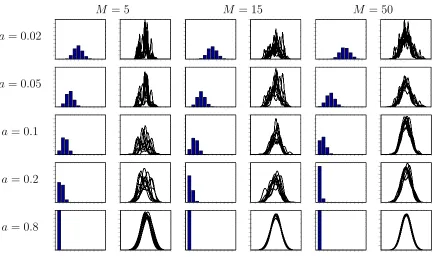
Figure 1: The prior distribution of the number of modes of F and a sample of densities under different hyperparameter choices
features of the realized distribution. The parameteracan be interpreted as a measure of local dependence (and so local variability) and the parameterM as measure of global variability. The figure also gives us an indication of the link betweenaand the modal number of modes. A values of abetween 0.1 and 0.2 indicates a prior belief of bi- or tri-modality wheareas a = 0.02 indicates support to a number of modes between 3 and 9. These observations are helpful for defining a variety of prior distributions ofa. The new prior distribution is a reparameterisation of the usual conjugate prior distribution wherea= n0
1+n0, which is usually
assumed fixed and small which implies unsmooth densities. The scaling is surprising since n0 = 0.01would be considered a large value but implies many modes. A notable exception
is Richardson and Green (1997) who defineH(µ, σ2) =N(ζ, κ−1)Ga(σ−2|α, β)in a finite
mixture model with a Gamma hyperprior onβ. Another interesting aspect of the prior is the importance of the role playedarelative toM in the realised distributions.
I will use various moments of the observables and the unknown distributionf to clarify, and quantify, the roles of the parameters. The constant component-specific variance can be generalized toσ2
kζi, where E[ζi] = 1 to allow greater flexibility. A standard choice is
an inverse gamma distribution forζi with shape parameterα and scale parameter 1, which
of parameters to be estimated in the model which we hope will lead to more tighly fitting model but a random effects specification for the variance can lead to a smaller number of components with certain data. A mixture distribution forζiwould define a compromise prior
p(ζi) =w δζ=1+ (1−w) (α−1)IG(α,1).
If we consider a more general form of mixture density forf f(x) =
∞
X
i=1
pik(x|µi, σk2, φ)
wherek is a symmetric probability density function with meanµi, variance σk2ζi and any
other parameters of the density function denoted byφ. Let the mean of the centring distribu-tionHbeµ0then the first two predictive central moments have the form
E[yi] =E[µi] =µ0, V[yi] =V[µi] +σk2E[ζi] =σ2
and the overall predictive variability can be divided into a component due to the variability within components and between components so that
V[µi] = (1−a)σ2, σ2k=
aσ2 E[ζi].
The predictive skewness have the form
E[(yi−µ0)3] =E[E[(yi−µi+µi−µ0)3|µi, σki2]]
=E[(yi−µi)3|µi] +E[(µi−µ0)3],
the sum of the within-component and between-component skewness, and the kurtosis can be expressed as
E[(yi−µ0)4] =E[E[(yi−µi+µi−µ0)4|µi]]
=E[E[(yi−µi)4|µi]] + 6a(1−a)σ4+E[(µi−µ0)4].
If both distributions are chosen to be normal then this expression equals3σ4. However
heav-ier tailed predictive distribution will arise through either changes to the component distrib-ution or, perhaps more usefully, the distribdistrib-ution of the component means. These properties are unaffected by the choice of by the choice of the species sampling model. Of course, the species sampling model will effect the variability in the moments of realized distribution. To consider the effect of the species sampling model and the parameter a, we look at the following quantity
Cov[f(x1), f(x2)] =C(x1, x2)
∞
X
i=1
a= 0.1 a= 0.2 a= 0.4 a= 0.7
0 0.5 1 1.5 2 2.5 3 3.5 0
0.05 0.1 0.15 0.2 0.25
0 0.5 1 1.5 2 2.5 3 3.5 0
0.02 0.04 0.06 0.08 0.1 0.12
0 0.5 1 1.5 2 2.5 3 3.5 0
0.005 0.01 0.015 0.02 0.025 0.03 0.035 0.04 0.045 0.05
0 0.5 1 1.5 2 2.5 3 3.5 0
[image:8.595.107.498.92.179.2]0.002 0.004 0.006 0.008 0.01 0.012 0.014 0.016 0.018 0.02
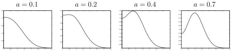
Figure 2:C(x1, x1)with a standard normal predictive distribution and various values ofa
where
C(x1, x2) =E[k(x1|µ, aσ2ζi, φ)k(x2|µ, aσ2ζi, φ)]−E[k(x1|µi, aσ2, ζi, φ)]E[k(x2|µi, aσ2, ζi, φ)].
The variability off(x1)is then
V[f(x1)] =C(x1, x1)
∞
X
i=1
E[p2i].
The first part of the product, C(x,x1), on the right-hand side is related to the choice ofk andaand the second part is related to the choice of species sampling model. If we use a Dirichlet process mixtureP∞i=1E[p2
i] = M1+1. Figure 2 showsC(x1, x1)when we assume
a standard normal predicive distribution in the mixture of normals model with various values ofa. The variability decreases as the value ofaincreases but a second effect is also clear: the variability will only be monotone decreasing inxfor small values of a. Consequently largearepresents a confidence in the density at the mean but less confidence in the density in the region around one standard deviation. An alternative measure, which underlies our understanding of the species sampling models themselves is the variability in the probability measure on a setBwhich can be expressed as
V[F(B)] =
Z
B
Z
B
C(x, y)dx dy.
The correlation between the density values at two points can be expressed as Corr[f(x1), f(x2)] = p C(x1, x2)
C(x1, x1)C(x2, x2)
.
a= 0.1 a = 0.2 a= 0.4 a= 0.7
0 0.5 1 1.5 2 2.5 3 3.5 0
0.5 1 1.5 2 2.5 3 3.5
0 0.5 1 1.5 2 2.5 3 3.5 0
0.5 1 1.5 2 2.5 3 3.5
0 0.5 1 1.5 2 2.5 3 3.5 0
0.5 1 1.5 2 2.5 3 3.5
0 0.5 1 1.5 2 2.5 3 3.5 0
[image:9.595.112.496.92.179.2]0.5 1 1.5 2 2.5 3 3.5
Figure 3: Prior correlation between the density values at two pointsx1 andx2 for a model with
a standard normal predictive distribution and various values ofawhere darker colours represent larger correlations
xare associated with much larger ranges (the distance at which the autocorrelation is equal to some small prespecified value). The autocorrelation between two setsB1 andB2can be
expressed as
Corr(F(B1), F(B2)] =
R
B1
R
B2C(x, y)dx dy
qR
B1
R
B1C(x, y)dx dy
R
B2
R
B2C(x, y)dx dy
=
Z
B1
Z
B2
w(x, y)Corr(f(x), f(y))dx dy where
w(x, y) =
s
C(x, x)C(y, y)
R
B1
R
B1C(x, y)dx dy
R
B2
R
B2C(x, y)dx dy
.
The measures considered in this section quantify the relationships that are evident from the figure 1. The parameteracontrols the local prior behaviour of the density function and, at least in the Dirichlet process case, the parameter of the species sampling model controls the general variability. It seems reasonable given the results on the variance and correlation of the density function to assume that these relationship will largely carry over to other species sampling models. The following section uses these ideas to develop prior distribution fora and the location and scale parametersµ0andσ2.
2.1 Prior distributions for the parameters of the model
One purpose of this paper is to suggest forms of prior for the mixture model that allow us to replace a parametric distribution, in this case the normal distribution, by a nonparametric alternative. In particular it would useful to maintain the same prior structure across these two possible specifications. There are two standard choices of prior forµ0 andσ2: the
im-proper choice of Jeffreys’ prior p(µ0, σ−2) ∝ σ2 and the conjugate choice p(µ0, σ−2) =
N(µ|µ00, φσ2)Ga(σ−2|α, β). The second choice always leads to a proper posterior
following result shows that the posterior distribution will always be proper. Robert and Tit-terington (1998) have previously considered a similar approach for a different prior in finite mixture models. They place Jeffreys’ prior distribution on the parameters of the first compo-nent and then allow the location and scale of thek-th cluster to depend on the locations and scales of the previousk−1components. This seems more suited to a finite mixture case for cluster analysis rather than density estimation problems where centring the predictive distri-bution over a particular parametric form seems a useful starting for prior specification. They observe that dependence between the priors on the parameters of each component is key to the use of improper priors for location and scale and the same is true for the prior proposed in this paper. It is simple to show posterior existence for the prior structure in this paper. In particular the posterior will exist if
p(y|µ0, σ2, a) =
Z σ−2
l
Y
i=1
Z
k(y|µi, ζi, a, σ2)h(µi|µ0, a, σ2)p(ζi)dµidζidµ0dσ2
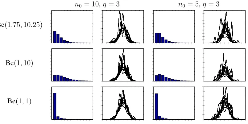
is finite, which is true for the the mixture of normals models considered in this paper. Finally, the prior specification for the smoothness parameteraand the parameters of the species sampling model is considered. In this paper, the choice of species sampling model will be restricted to the Dirichlet process and a prior distribution for the mass parameterM is proposed. The form of the prior distribution ofais restricted to follow a Beta distribution and several possible parameter choices are considered. The prior distribution of the nonpara-metric part is defined through a prior distribution forζ =P∞i=1E[p2i]with the density
p(ζ) =nη0 Γ(2η)
(Γ(η))2
[ζ(1−ζ)]η−1
[(n0−1)ζ+ 1]2η.
In the Dirichlet process case, whereζ = 1
M+1, the properties of this prior distribution are
discussed by Griffin and Steel (2004).
n0 = 10,η = 3 n0 = 5,η= 3
Be(1.75,10.25)
1 2 3 4 5 6 7 8 9 101112 0
0.1 0.2 0.3 0.4 0.5 0.6 0.7 0.8 0.9 1
−5 −4 −3 −2 −1 0 1 2 3 4 5 0
0.2 0.4 0.6 0.8 1 1.2 1.4 1.6 1.8
1 2 3 4 5 6 7 8 9 101112 0
0.1 0.2 0.3 0.4 0.5 0.6 0.7 0.8 0.9 1
−5 −4 −3 −2 −1 0 1 2 3 4 5 0
0.2 0.4 0.6 0.8 1 1.2 1.4 1.6 1.8 2
Be(1,10)
1 2 3 4 5 6 7 8 9 101112 0
0.1 0.2 0.3 0.4 0.5 0.6 0.7 0.8 0.9 1
−5 −4 −3 −2 −1 0 1 2 3 4 5 0
0.5 1 1.5 2 2.5
1 2 3 4 5 6 7 8 9 101112 0
0.1 0.2 0.3 0.4 0.5 0.6 0.7 0.8 0.9 1
−5 −4 −3 −2 −1 0 1 2 3 4 5 0
0.5 1 1.5 2 2.5 3 3.5
Be(1,1)
1 2 3 4 5 6 7 8 9 101112 0
0.1 0.2 0.3 0.4 0.5 0.6 0.7 0.8 0.9 1
−5 −4 −3 −2 −1 0 1 2 3 4 5 0
0.5 1 1.5 2 2.5 3 3.5
1 2 3 4 5 6 7 8 9 101112 0
0.1 0.2 0.3 0.4 0.5 0.6 0.7 0.8 0.9 1
−5 −4 −3 −2 −1 0 1 2 3 4 5 0
[image:11.595.106.508.93.294.2]0.5 1 1.5 2 2.5 3 3.5
Figure 4: The prior distribution of the number of modes of F and a sample of densities under different hyperparameter choices
2.2 Multivariate versions
The ideas described up to this point relate to univariate density estimation. However, the multivariate problem is important and has received particularly attention in the Bayesian literature on random effects model where the distribution of the random effects is to be es-timated (seee.g. M¨uller and Rosner 1997). The smoothness parameterain the univariate case defines the proportion of the overall variance assigned to within component variation. There is no single natural extension to the multivariate case but there are two natural starting points: the orientation of the observed vectors has some meaning or the orientation of the ob-served vectors is essentially arbitary (in which case we would be happy to rotate axis without affecting the analysis). In both case the univariate model is extended by assuming that the mean of data isµ0 and the covariance matrix isΣ. In the first case, we want to respect the dimension of the variables and to have different smoothness parameter (values ofa)for each dimension. The choice of within-component covariance matrixΣksuch that
Σkij =√aiajΣij
implies that the correlation between thei-th andj-th variable is √Σij
ΣiiΣjj. This define Model I which allows different levels of departure from the centring model in different dimension and the prior for the marginal distibution of thei-th variable will the univariate model with smoothing parameter ai. The prior covariance matrix of the µi will then have the form
a = 0.02 a= 0.2 a= 0.8
a = 0.02 −5−5 −4−3 −2 −1 0 1 2 3 4 5 −4 −3 −2 −1 0 1 2 3 4 5
−5 −4 −3−2 −1 0 1 2 3 4 5 −5 −4 −3 −2 −1 0 1 2 3 4 5
−5 −4−3 −2 −1 0 1 2 3 4 5 −5 −4 −3 −2 −1 0 1 2 3 4 5
−5 −4 −3−2 −1 0 1 2 3 4 5 −5 −4 −3 −2 −1 0 1 2 3 4 5
−5−4 −3−2 −1 0 1 2 3 4 5 −5 −4 −3 −2 −1 0 1 2 3 4 5
−5−4 −3−2 −1 0 1 2 3 4 5 −5 −4 −3 −2 −1 0 1 2 3 4 5
−5−4 −3−2 −1 0 1 2 3 4 5 −5 −4 −3 −2 −1 0 1 2 3 4 5
−5−4 −3−2 −1 0 1 2 3 4 5 −5 −4 −3 −2 −1 0 1 2 3 4 5
−5−4 −3−2 −1 0 1 2 3 4 5 −5 −4 −3 −2 −1 0 1 2 3 4 5
−5−4 −3−2 −1 0 1 2 3 4 5 −5 −4 −3 −2 −1 0 1 2 3 4 5
−5−4 −3−2 −1 0 1 2 3 4 5 −5 −4 −3 −2 −1 0 1 2 3 4 5
−5−4 −3−2 −1 0 1 2 3 4 5 −5 −4 −3 −2 −1 0 1 2 3 4 5
a= 0.2 −5−5 −4−3 −2 −1 0 1 2 3 4 5 −4 −3 −2 −1 0 1 2 3 4 5
−5 −4 −3−2 −1 0 1 2 3 4 5 −5 −4 −3 −2 −1 0 1 2 3 4 5
−5 −4−3 −2 −1 0 1 2 3 4 5 −5 −4 −3 −2 −1 0 1 2 3 4 5
−5 −4 −3−2 −1 0 1 2 3 4 5 −5 −4 −3 −2 −1 0 1 2 3 4 5
−5−4 −3−2 −1 0 1 2 3 4 5 −5 −4 −3 −2 −1 0 1 2 3 4 5
−5−4 −3−2 −1 0 1 2 3 4 5 −5 −4 −3 −2 −1 0 1 2 3 4 5
−5−4 −3−2 −1 0 1 2 3 4 5 −5 −4 −3 −2 −1 0 1 2 3 4 5
−5−4 −3−2 −1 0 1 2 3 4 5 −5 −4 −3 −2 −1 0 1 2 3 4 5
−5−4 −3−2 −1 0 1 2 3 4 5 −5 −4 −3 −2 −1 0 1 2 3 4 5
−5−4 −3−2 −1 0 1 2 3 4 5 −5 −4 −3 −2 −1 0 1 2 3 4 5
−5−4 −3−2 −1 0 1 2 3 4 5 −5 −4 −3 −2 −1 0 1 2 3 4 5
−5−4 −3−2 −1 0 1 2 3 4 5 −5 −4 −3 −2 −1 0 1 2 3 4 5
a= 0.8 −5−5 −4−3 −2 −1 0 1 2 3 4 5 −4 −3 −2 −1 0 1 2 3 4 5
−5 −4 −3−2 −1 0 1 2 3 4 5 −5 −4 −3 −2 −1 0 1 2 3 4 5
−5 −4−3 −2 −1 0 1 2 3 4 5 −5 −4 −3 −2 −1 0 1 2 3 4 5
−5 −4 −3−2 −1 0 1 2 3 4 5 −5 −4 −3 −2 −1 0 1 2 3 4 5
−5−4 −3−2 −1 0 1 2 3 4 5 −5 −4 −3 −2 −1 0 1 2 3 4 5
−5−4 −3−2 −1 0 1 2 3 4 5 −5 −4 −3 −2 −1 0 1 2 3 4 5
−5−4 −3−2 −1 0 1 2 3 4 5 −5 −4 −3 −2 −1 0 1 2 3 4 5
−5−4 −3−2 −1 0 1 2 3 4 5 −5 −4 −3 −2 −1 0 1 2 3 4 5
−5−4 −3−2 −1 0 1 2 3 4 5 −5 −4 −3 −2 −1 0 1 2 3 4 5
−5−4 −3−2 −1 0 1 2 3 4 5 −5 −4 −3 −2 −1 0 1 2 3 4 5
−5−4 −3−2 −1 0 1 2 3 4 5 −5 −4 −3 −2 −1 0 1 2 3 4 5
[image:12.595.70.534.94.394.2]−5−4 −3−2 −1 0 1 2 3 4 5 −5 −4 −3 −2 −1 0 1 2 3 4 5
Figure 5: Four realisations of the multivariate model 1 with different value ofacorrelation 0 with
M = 5
zi = A−1(yi −µ0) where A is the Choleksy decomposition ofΣ and the distribution of
zi will be centred over a multivariate standard normal. The within component covariance
matrix is assumed to have the form
Σk=
a1 . .. ap .
and the between component covariance is assumed to be
Σ0 =
1−a1
. ..
1−ap
.
give rise to distribution with less modes and a more cohesive distribution. As in the univariate case, it is also possible to define a version where each cluster variance is different. Let
E(yi|µi, σ2) =µi, V(yi|µi, σ2) = Σkζi
whereζiis a distribution with the indentity as the mean. Standard choices such a the inverted
Wishart distribution can fit into this structure.
a = 0.02 a= 0.2 a= 0.8
a = 0.02 −5−5 −4−3 −2 −1 0 1 2 3 4 5 −4 −3 −2 −1 0 1 2 3 4 5
−5 −4 −3−2 −1 0 1 2 3 4 5 −5 −4 −3 −2 −1 0 1 2 3 4 5
−5 −4−3 −2 −1 0 1 2 3 4 5 −5 −4 −3 −2 −1 0 1 2 3 4 5
−5 −4 −3−2 −1 0 1 2 3 4 5 −5 −4 −3 −2 −1 0 1 2 3 4 5
−5−4 −3−2 −1 0 1 2 3 4 5 −5 −4 −3 −2 −1 0 1 2 3 4 5
−5−4 −3−2 −1 0 1 2 3 4 5 −5 −4 −3 −2 −1 0 1 2 3 4 5
−5−4 −3−2 −1 0 1 2 3 4 5 −5 −4 −3 −2 −1 0 1 2 3 4 5
−5−4 −3−2 −1 0 1 2 3 4 5 −5 −4 −3 −2 −1 0 1 2 3 4 5
−5−4 −3−2 −1 0 1 2 3 4 5 −5 −4 −3 −2 −1 0 1 2 3 4 5
−5−4 −3−2 −1 0 1 2 3 4 5 −5 −4 −3 −2 −1 0 1 2 3 4 5
−5−4 −3−2 −1 0 1 2 3 4 5 −5 −4 −3 −2 −1 0 1 2 3 4 5
−5−4 −3−2 −1 0 1 2 3 4 5 −5 −4 −3 −2 −1 0 1 2 3 4 5
a= 0.2 −5−5 −4−3 −2 −1 0 1 2 3 4 5 −4 −3 −2 −1 0 1 2 3 4 5
−5 −4 −3−2 −1 0 1 2 3 4 5 −5 −4 −3 −2 −1 0 1 2 3 4 5
−5 −4−3 −2 −1 0 1 2 3 4 5 −5 −4 −3 −2 −1 0 1 2 3 4 5
−5 −4 −3−2 −1 0 1 2 3 4 5 −5 −4 −3 −2 −1 0 1 2 3 4 5
−5−4 −3−2 −1 0 1 2 3 4 5 −5 −4 −3 −2 −1 0 1 2 3 4 5
−5−4 −3−2 −1 0 1 2 3 4 5 −5 −4 −3 −2 −1 0 1 2 3 4 5
−5−4 −3−2 −1 0 1 2 3 4 5 −5 −4 −3 −2 −1 0 1 2 3 4 5
−5−4 −3−2 −1 0 1 2 3 4 5 −5 −4 −3 −2 −1 0 1 2 3 4 5
−5−4 −3−2 −1 0 1 2 3 4 5 −5 −4 −3 −2 −1 0 1 2 3 4 5
−5−4 −3−2 −1 0 1 2 3 4 5 −5 −4 −3 −2 −1 0 1 2 3 4 5
−5−4 −3−2 −1 0 1 2 3 4 5 −5 −4 −3 −2 −1 0 1 2 3 4 5
−5−4 −3−2 −1 0 1 2 3 4 5 −5 −4 −3 −2 −1 0 1 2 3 4 5
a= 0.8 −5−5 −4−3 −2 −1 0 1 2 3 4 5 −4 −3 −2 −1 0 1 2 3 4 5
−5 −4 −3−2 −1 0 1 2 3 4 5 −5 −4 −3 −2 −1 0 1 2 3 4 5
−5 −4−3 −2 −1 0 1 2 3 4 5 −5 −4 −3 −2 −1 0 1 2 3 4 5
−5 −4 −3−2 −1 0 1 2 3 4 5 −5 −4 −3 −2 −1 0 1 2 3 4 5
−5−4 −3−2 −1 0 1 2 3 4 5 −5 −4 −3 −2 −1 0 1 2 3 4 5
−5−4 −3−2 −1 0 1 2 3 4 5 −5 −4 −3 −2 −1 0 1 2 3 4 5
−5−4 −3−2 −1 0 1 2 3 4 5 −5 −4 −3 −2 −1 0 1 2 3 4 5
−5−4 −3−2 −1 0 1 2 3 4 5 −5 −4 −3 −2 −1 0 1 2 3 4 5
−5−4 −3−2 −1 0 1 2 3 4 5 −5 −4 −3 −2 −1 0 1 2 3 4 5
−5−4 −3−2 −1 0 1 2 3 4 5 −5 −4 −3 −2 −1 0 1 2 3 4 5
−5−4 −3−2 −1 0 1 2 3 4 5 −5 −4 −3 −2 −1 0 1 2 3 4 5
[image:13.595.69.533.203.500.2]−5−4 −3−2 −1 0 1 2 3 4 5 −5 −4 −3 −2 −1 0 1 2 3 4 5
Figure 6: Four realisations of the multivariate model 1 with different value ofa correlation 0.5 withM = 5
3 Computational methods
mixture models described in Papaspiliopoulos and Roberts (2004), which uses a finite trunca-tion ofGwhilst avoiding truncation error. This allows direct posterior inference forfandG. Alternatively, Gelfand and Kottas (2002) describe methods for making inference about these objects using marginal methods. Discussion of computational methods is not the purpose of this paper and the reader is referred to Papaspiliopoulos and Roberts (2004) for comparison of the various methods. All methods make use of the Gibbs sampler and the full conditional distribution for each parameter are fully described in each paper. This section describes meth-ods for sampling any unusual full conditional distributions. Before describing these steps it is important to note that in all the methods, thei-th observations is allocated to a compo-nent value(µsi, σ2si), which leads to simple forms for many full conditional distributions in a Gibbs sampling scheme.
3.1 Updating
M
Mcan be updated using an independence Metropolis-Hastings sampler. The Newton-Raphson method is used to find the mode of the full conditional distribution, then the proposal dis-tribution is at-distribution centred at the mode, with α degrees of freedom and precision parameterλ= α
α+1×-Hessian. A default choice ofαwould be 3.
3.2 Updating
σ
2k
and
σ
02in the normal model
To updatea, σ2, we transform back toσ2
kandσ20 whereσ2 =σk2+σ02anda= σ
2
k
σ2
k+σ20. The
jacobian of the transformation isσ21
k+σ20. The transformed prior is
p(σk2, σ02) = 1
σ2
k+σ02
pa
µ σk2 σ2
k+σ20
pσ2(σ2k+σ20).
Ifσ2has an improper prior, we use a rejection sampler with the envelope
σk2 ∼IG Ã
n/2 +βˆa−(1−aˆ)α,1
2
n
X
i=1
(yi−θsi)2
!
σ02∼IG Ã
k/2 +α(1−ˆa)−βˆa,1
2
k
X
i=1
(θi−µ0)2
!
whereˆais the current value of σ2k
σ2
0+σ2k. The acceptance probability is
1 (σ2
k+σ20)α+β
µ σ2k
ˆ
a
¶(α+β)ˆaµ
σ2 0
1−ˆa
In the proper case, whereσ2follows an inverted Gamma distribution with shapecand scale d, we define the joint distribution
σk2 ∼IG Ã
n/2 + (β+c)ˆa−(1−ˆa)α,1
2
n
X
i=1
(yi−θsi)
2+dˆa2
!
σ02 ∼IG Ã
k/2 + (α+c)(1−ˆa)−βa,ˆ 1 2
k
X
i=1
(θi−µ0)2+d(1−ˆa)2
!
which can be used as a proposal distribution in a Metropolis-Hasting sampler which has acceptance probability
min
1, µ
σ02 ˆa kσ021
−ˆa
0
σ02
k+σ020
¶α+β+c
exp
n −d
h
1
σ02
k+σ020 −
ˆ
a σ02
k −
1−ˆa
σ02 0
io µ
σ2 ˆa kσ210−ˆa
σ2
k+σ20
¶α+β+c
exp
n −d
h
1
σ2
k+σ02 −
ˆ
a σ2
k −
1−aˆ
σ2 0
io
whereσ02
kandσ020represent the proposed values ofσ2kandσ20respectively.
3.2.1 Updatingζi
Ifζi ∼IG(α, β)then
ζi∼IG
Ã
α+ 0.5ni,1 + 0.5
P
j|sj=i(xj−µi)
2
(α−1)aσ2
!
Updatinga andσ2 use the rejection sampler from above replacing Pj|sj=i(xj −µi)2 by
1
(α−1)ζi
P
j|sj=i(xj−µi)
2.
3.3 Multivariate extensions
3.3.1 UpdatingΣanda
For both models described in section 2.2, these parameters can be updated using a random walk Metropolis-Hastings with normal proposals whose variance have been tuned to achieve an acceptance rate close to 0.234.
4 Examples
4.1 Univariate density estimation
and introduced into the Bayesian literature by Roeder and Wassermann (1997). It has be-come a standard data set for the comparison of Bayesian density estimation models and their related computational algorithms. The data records the estimated velocity (×10−2) at which
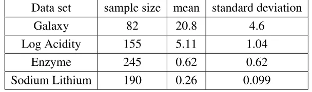
82 galaxies are moving away from our galaxy. Some galaxies are thought to be moving at similar speeds whilst other move much faster or slower. Inferring the clusters of galaxy is the main inferential problem. Of course, this rather contradict the basis of this paper and the problem here is treated as density estimation (in common with much of the subsequent literature). However, if the clusters are not assumed normal then modality of the data may give some clue to the various groupings. The “acidity” data refers to a sample of 155 acidity index measurement made on linkes in noth-central Wisconsin which are analysed on the log scale, the “enzyme” data measures the enzymatic activity in the blood of 245 unrelated indi-viduals. It is hypothesised that there are groups of slow and fast metabolizers. These three data sets were previously analysed in Richardson and Green (1997). A final data records the red blood cell sodium-lithium countertransport (SLC) in six large English kindreds. The data was previously analysed by Roeder (1994) who wants to distinguish between a two and three component finite mixture, which she postulates will have the same variance. Further back-ground to the genetic implications of different types of multi-modality are explained in the reference. Some summary statistics for the four data sets are shown in table 1. In all analyses the prior forM is set to have hyperparametersn0 = 5andη = 3andζi ∼ IG(2,1). Two
prior choices forawere chosen: Be(1,10)and Be(1,1)which represent a prior distribution with substantial prior mass on a wide range of modes and prior distribution that places a lot of a mass on a single mode.
Data set sample size mean standard deviation
Galaxy 82 20.8 4.6
Log Acidity 155 5.11 1.04
Enzyme 245 0.62 0.62
[image:16.595.150.454.462.552.2]Sodium Lithium 190 0.26 0.099
Table 1: Summary statistics for the 4 data sets
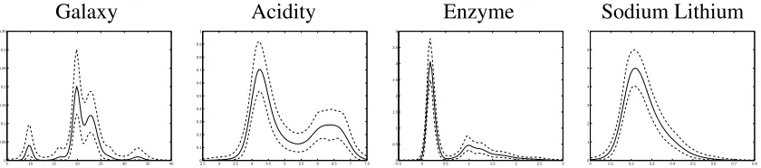
Galaxy Acidity Enzyme Sodium Lithium
5 10 15 20 25 30 35 40 0
0.05 0.1 0.15 0.2 0.25 0.3 0.35
2.5 3 3.5 4 4.5 5 5.5 6 6.5 7 7.5 0
0.1 0.2 0.3 0.4 0.5 0.6 0.7 0.8 0.9 1
−0.50 0 0.5 1 1.5 2 2.5 3 0.5
1 1.5 2 2.5 3 3.5 4
0 0.1 0.2 0.3 0.4 0.5 0.6 0.7 0.8 0
[image:17.595.95.515.93.186.2]1 2 3 4 5 6 7
Figure 7: Posterior predictive densities for the four data sets with a pointwise95%HPD interval
a number of other analysese.g. Richardson and Green (1997).
Table 2 shows summaries of the posterior distributions ofaandM under the two prior distributions ofa. The parameterahas been interpreted as the smoothness of the realised dis-tribution and related to the number of posterior modes. The results show that the disdis-tribution which are less smooth (in particular the multi-modal galaxy data) have smaller estimates of a, which is estimated with good precision in each case. Unsurprisingly the unimodal distri-bution of sodium lithium has the highest estimates ofa. The posterior distribution is robust to the choice between the two prior distribution when the density are estimated to be less smooth. For distributions which have higher levels of smoothness the prior distribution is much more influential. This mostly shows a prior-likelihood mismatch since the tighter prior distribution places nearly at its mass below 0.2 and neglible mass above 0.3. Clearly under the more dispersed prior distribution the posterior distribution for the acidity and sodium lithium data sets place mass at larger values. This suggests that a dispersed prior distribution will be useful when we are unsure about the smoothness and likely modality of the data. The posterior inferences ofMfor each data set show only small differences between the posterior median and credibility intervals, illustrating that differences in modality will not be captured in these models by theMparameters. The results for the number of clusters (not shown) also display a lack of difference in the form of the posterior distribution across the different data sets.
a M
Data set Be(1,1) Be(1,10) Be(1,1) Be(1,10)
Galaxy 0.04 (0.01, 0.12) 0.03 (0.01, 0.10) 3.73 (1.14, 10.80) 3.93 (1.31, 10.06) Acidity 0.16 (0.04, 0.46) 0.10 (0.03, 0.27) 3.47 (0.95, 10.66) 3.23 (0.83, 9.48) Enzyme 0.06 (0.01, 0.23) 0.05 (0.01, 0.16) 2.40 (0.75, 6.40) 2.39 (0.69, 7.31) Sodium Lithium 0.44 (0.12, 0.82) 0.17 (0.04, 0.41) 3.71 (0.79, 15.01) 2.25 (0.49, 6.69)
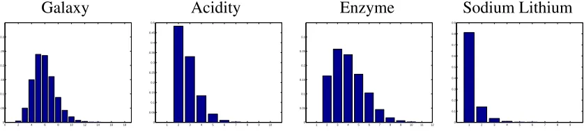
Galaxy Acidity Enzyme Sodium Lithium
0 2 4 6 8 10 12 14 16 18 0
0.05 0.1 0.15 0.2 0.25 0.3
1 2 3 4 5 6 7 8 9 10 0
0.05 0.1 0.15 0.2 0.25 0.3 0.35 0.4 0.45 0.5
1 2 3 4 5 6 7 8 9 10 11 12 0
0.05 0.1 0.15 0.2 0.25 0.3
1 2 3 4 5 6 7 8 9 0
[image:18.595.95.514.94.188.2]0.1 0.2 0.3 0.4 0.5 0.6 0.7 0.8 0.9
Figure 8: Posterior predictive densities for the four data sets
The inferences about the number of modes is shown in figure 8. The degree of posterior uncertainty for most of the data sets (with the exception of sodium lithium) is substantial and is obscured in the posterior predictive distributions. In all cases the results are shown for Be(1,1)prior, as witha, the results are unchanged with the second prior for the galaxy and enzyme data. The galaxy data supports a range of values between 3 and 9. The values 5 and 6 receive almost equal posterior support. The acidity data shows strongest support for 2 modes and some uncertainty about and extra 1 or 2 modes. The enzyme data also shows a large amount of posterior uncertainty about the number of modes. It show most support for 3 modes with good support for upto 7 modes. The results are rather surprising given the shape of the posterior predictive distribution. It seems reasonable to conjecture that the form of the model may lead to these results. The data can be roughly divided into two groups. The skewness of the second group can only be captured by a number of normal distribution. This may lead to rather unrealistic estimates of the number of modes. The sodium lithium data set results are shown for the Be(1,1)prior. The posterior distribution strongly supports a single mode with a posterior probability of about 0.8.
4.2 Multivariate data example
As an example, I re-analyse a data set, previously analysed by Bowman and Azzalini (1997), that relates to a study of the development of aircraft technology originally analysed by Saviotti and Bowman (1984). The data set contain six characteristics (total engine power, wing span, length, maximum take-off weight, maximum speed and range) of aircraft de-signs. The first two principal components are shown in figure and can be interpreted as “size” and “speed adjusted for size”. Further details are given in the reference. A Beta(1,1) prior distribution was used fora1 anda2. The prior distribution ofΣwas chosen to be an
inverse Wishart distribution with 3 degrees of freedom and the prior mean fixed to the sample covariance matrix. The data is analysed using Model I to illustrate the methodology although Model II seems more appropriate in this application.
parameter median 95% credible interval
a1 0.103 (0.078, 0.137)
[image:19.595.192.416.90.145.2]a2 0.095 (0.086, 0.140)
Table 3: Summary of the posterior distribution ofa1anda2 for the aircraft data
similar level of non-normality in both variables. Once again both parameter are estimated to a good level of certainty. Figure 9 shows a scatterplot of the data and the posterior predictive distribution for the chosen prior. The predictive distribution gives a good description of the data. In particular, the higher density of points on the for smallx1is well captured and gives
similar results to Bowman and Azzalin (1997).
(a) (b)
−6 −4 −2 0 2 4 6 8
−3 −2 −1 0 1 2 3 4
principal component 1
principal component 2
−4 −3 −2 −1 0 1 2 3 4 5 6 7 −3
−2 −1 0 1 2 3
Figure 9: Aircraft data: (a) a scatterplot of the data and (b) a heatplot of the posterior predictive density function where darker colours represent higher density values
5 Discussion
This paper presents an alternative interpretation of the species sampling mixture of normals model often used for Bayesian density estimation which contrast with the more usual subpop-ulation motivation. The unknown density,f, is treated as the main parameter of interest and prior information is consequently placed directly onto this object. This naturally leads to an alternative parameterisation and prior distribution that are, in certain situations, much easier to specify than previously defined models. It is usual to fixn0in the standard conjugate prior
distribution and define a value ofσ2related to the overall variability in the data. In univariate
[image:19.595.156.453.275.409.2]modes. Recent developments in computational methods for non-conjugate Dirichlet process and general stick-breaking prior distribution (Neal 2000, Neal and Jain 2006, Papaspiliopou-los and Roberts 2004) make these ideas feasible. However, in common with many other Bayesian methods, non-informative prior distributions can lead to posterior distributions for σ2 which have long tails. Use of prior information about the location and scale will lead to
more concentrated posterior distributions which may be preferable in a some applications. However, the automatic nature of improper priors is often appealing.
This paper has concentrated on density estimation of distributions of observables but many Bayesian applications of nonparametric density estimation of unobservable quantities, such as random effects. The approach developed here can play a more important role in these problems where choices of scale for the component and the distribution of the component means will be hard to choose in many practical applications. The specification describe in this paper allows us to replace a parametric distribution by a nonparametric specification of f whilst retaining the other structure of the parametric model. For example, the univariate analyses presented in this paper directly generalize the standard Bayesian normal model with Jeffreys’ prior for the location and scale.
This paper has been restriced mostly to the Dirichlet process mixture of normals model which has been used extensively in the practical applications of Bayesian nonparametric methods. This paper could be generalized in a number of ways. A number of alternative species sampling models have been considered and it would be interesting to see the effect of alternative species sampling models on the inference. An alternative generalisation consider changing either the component specific distribution from normal or, perhaps more usefully, the centring distribution off. The results in section 2 suggest that the former idea will lead to different prior correlation structures for the density function. Other centring distribution are also possible. A simple method assumes that some lower order prior predictive moments off are fixed to coincide with those of a parametric distribution. For example, we could replace att-distribution with a mixture of normals where the the mean of the normals are also drawn from at-distribution. The results in section 2 make the link between the skewness and kurtosis of the various distributionss explicit.
References
Blackwell, D. and MacQueen, J.B. (1973): “Ferguson distributions via P´olya urn schemes,”
Annals of Statistics, 1, 353-355.
Bush, C. A. and S. N. MacEachern (1996): “A Semiparametric Bayesian Model for Ran-domised Block Designs,”Biometrika, 83, 275-285.
Escobar, M. D. and West, M. (1995): “Bayesian density-estimation and inference using mixtures,”Journal of the American Statistical Association, 90, 577-588 .
Ferguson, T. S. (1973): “A Bayesian Analysis of Some Nonparametric Problems,” The
Annals of Statistics, 1, 209-230.
Ferguson, T. S. (1983): “Bayesian Density Estimation by Mixtures of Normal Distribution,”
inRecent Advances In Statistics: Papers in Honor of Herman Chernoff on His Sixtieth
Birthday, eds: M. H. Rizvi, J. Rustagi and D. Siegmund, Academic Press: New York.
Gelfand, A. E. and A. Kottas (2002): “A Computational Approach for Full Nonparametric Bayesian Inference under Dirichlet Proces Mixture Models,”Journal of Computational
and Graphical Statistics, 11, 289-305.
Ishwaran, H. and James, L. (2001): “Gibbs Sampling Methods for Stick-Breaking Priors,”
Journal of the American Statistical Association, 96, 161-73.
Ishwaran, H. and James, L. F. (2002): “Approximate Dirichlet Process Computing in Finite Normal Mixtures: Smoothing and Prior Information,”Journal of Computational and
Graphical Statistics, 11, 1-26.
Jain, S. and R. M. Neal (2005): “Splitting and merging components of a nonconjugate Dirichlet process mixture model,” Technical Report 0507, Department of Statistics, University of Toronto.
James, L. F. (2006): “Spatial neutral to the right species sampling mixture models,” pre-pared for “Festschrift for Kjell Doksum”.
Lijoi, A., R. H. Mena, and I. Pr¨unster (2005): “Hierarchical mixture modelling with nor-malized inverse-Gaussian priors,”Journal of the American Statistical Association, 100, 1278-1291./par
Lo, A. Y. (1984): “On a Class of Bayesian Nonparametric Estimates: I. Density Estimates,”
The Annals of Statistics, 12, 351-357.
MacEachern, S. N. and M¨uller, P. (1998): “Estimating mixture of Dirichlet process models,”
Journal of Computational and Graphical Statistics, 7, 223-238.
M¨uller, P. and Quintana, F. (2004): “Nonparametric Bayesian Data Analysis,”Statistical
Science, 19, 95-110.
M¨uller, P. and Rosner, G. (1997): “A Bayesian population model with hierarchical mixture priors applied to blood count data,” Journal of the American Statistical Association, 92, 1279-1292.
Neal, R. M. (2000): “Markov chain sampling methods for Dirichlet process mixture mod-els,”Journal of COmputational and Graphical Statistics, 9, 249-265.
Nietro-Barajas, L. E., I Pr¨unster and S. G. Walker (2004): “Normalized random measures driven by increasing additive processes,”Annals of Statistics, 32, 2343-2360.
Papaspiliopoulos, O. and Roberts, G. (2004): “Retrospective MCMC for Dirichlet process hierarchical models,” technical report, University of Lancaster.
Pitman, J. (1996): “Some Developments of the Blackwell-MacQueen Urn Scheme,” in
Statistics, Probability and Game Theory: Papers in Honor of David Blackwell, eds:
T. S. Ferguson, L. S. Shapley and J. B. MacQueen, Institue of Mathematical Statistics Lecture Notes.
Richardson, S. and P. J. Green (1997): “On Bayesian analysis of mixtures with unknown number of components (With discussion,”Journal of the Royal Statistical Society B, 731-792.
Robert, C. and M. Titterington (1998): “Reparameterisation strategies for hidden Markov models and Bayesian approaches to maximum likelihood estimation,” Statistics and
Computing, 4, 327-355.
Roeder, K. (1990): “Density Estation with Confidence Sets Exemplified by Superclusters and Voids in the Galaxies,”Journal of the American Statistical Assocation, 85, 617-624.
Roeder, K. (1994): “A Graphical Technique for Deteremining the Number of Components in a Mixture of Normals,”Journal of the American Statistical Assocation, 89, 487-495. Roeder, K. and L. Wasserman (1997): “Practical Bayesian Density Estimation Using
Mix-tures of Normals,”Journal of the American Statistical Association, 92, 894-902. Walker, S. G., Damien, P., Laud, P. W. and Smith, A. F. M. (1999): “Bayesian nonparametric
inference for random distributions and related functions,” (with discussion)Journal of