warwick.ac.uk/lib-publications
Original citation:
Bhattacharya, Sayan, Henzinger, Monika and Italiano, Giuseppe F. (2015) Deterministic fully
dynamic data structures for vertex cover and matching. In: Twenty-Sixth Annual ACM-SIAM
Symposium on Discrete Algorithms, San Diego, 4-6 Jan 2015. Published in: Proceedings of
the Twenty-Sixth Annual ACM-SIAM Symposium on Discrete Algorithms pp. 785-804.
Permanent WRAP URL:
http://wrap.warwick.ac.uk/92706
Copyright and reuse:
The Warwick Research Archive Portal (WRAP) makes this work of researchers of the
University of Warwick available open access under the following conditions. Copyright ©
and all moral rights to the version of the paper presented here belong to the individual
author(s) and/or other copyright owners. To the extent reasonable and practicable the
material made available in WRAP has been checked for eligibility before being made
available.
Copies of full items can be used for personal research or study, educational, or not-for-profit
purposes without prior permission or charge. Provided that the authors, title and full
bibliographic details are credited, a hyperlink and/or URL is given for the original metadata
page and the content is not changed in any way.
Publisher’s statement:
First Published in Proceedings of the Twenty-Sixth Annual ACM-SIAM Symposium on
Discrete Algorithm, 2015. published by the Society for Industrial and Applied Mathematics
(SIAM). Copyright © by SIAM. Unauthorized reproduction of this article is prohibited.
A note on versions:
The version presented in WRAP is the published version or, version of record, and may be
cited as it appears here.
Deterministic Fully Dynamic Data Structures
for Vertex Cover and Matching
Sayan Bhattacharya
∗Monika Henzinger
†Giuseppe F. Italiano
‡Abstract
We present the first deterministic data structures for main-taining approximate minimum vertex cover and maximum matching in a fully dynamic graph in o(√m) time per up-date. In particular, for minimum vertex cover we provide deterministic data structures for maintaining a (2 +) ap-proximation inO(logn/2) amortized time per update. For maximum matching, we show how to maintain a (3 +) ap-proximation inO(m1/3/2)amortizedtime per update, and a (4 +) approximation inO(m1/3/2)worst-casetime per up-date. Our data structure for fully dynamic minimum vertex cover is essentially near-optimal and settles an open problem by Onak and Rubinfeld [13].
1 Introduction
Finding maximum matchings and minimum vertex cov-ers in undirected graphs are classical problems in combi-natorial optimization. LetG= (V, E) be an undirected graph, with m = |E| edges and n = |V| nodes. A matching in G is a set of vertex-disjoint edges, i.e., no two edges share a common vertex. A maximum match-ing, also known as maximum cardinality matching, is a matching with the largest possible number of edges. A matching is maximal if it is not a proper subset of any other matching inG. A subsetV0⊆V is avertex cover if each edge ofGis incident to at least one vertex inV0. A minimum vertex cover is a vertex cover of smallest possible size.
The Micali-Vazirani algorithm for maximum
match-∗University of Vienna, Faculty of Computer Science. Email:
[email protected]. The research leading to these results has received funding from the European Research Council under the European Union’s Seventh Framework Programme (FP/2007-2013) / ERC Grant Agreement no. 340506.
†University of Vienna, Faculty of Computer Science. Email:
monika.henzinger at univie.ac.at. The research leading to these results has received funding from the European Research Council under the European Union’s Seventh Framework Pro-gramme (FP/2007-2013) / ERC Grant Agreement no. 340506.
‡Universit`a di Roma ”Tor Vergata”, Rome, Italy. Email:
[email protected]. Partially supported by MIUR, the Italian Ministry of Education, University and Research, under Project AMANDA (Algorithmics for MAssive and Networked DAta).
ing runs inO(m√n) time [5, 10]. Using this algorithm, a (1 +)-approximate maximum matching can be con-structed inO(m/) time [3]. Finding a minimum vertex cover, on the other hand, is NP-hard. Still, these two problems remain closely related as their LP-relaxations are duals of each other. Furthermore, a maximal match-ing, which can be computed in O(m) time in a greedy fashion, is known to provide a 2-approximation both to maximum matching and to minimum vertex cover (by using the endpoints of the maximal matching). Under the unique games conjecture, the minimum vertex cover cannot be efficiently approximated within any constant factor better than 2 [7]. Thus, under the unique games conjecture, the 2-approximation in O(m) time by the greedy method is the optimal guarantee for this prob-lem.
In this paper, we consider a dynamic setting, where the input graph is being updated via a sequence of edge insertions/deletions. The goal is to design data structures that are capable of maintaining the solution to an optimization problem faster than recomputing it from scratch after each update. If P 6= N P we can-not achieve polynomial time updates for minimum ver-tex cover. We also observe that achieving fast update times for maximum matching appears to be a partic-ularly difficult task: in this case, an update bound of
O(polylog(n)) would be a breakthrough, since it would immediately improve the longstanding bounds of the static algorithms [5, 9, 10, 11]. The best known update bound for dynamic maximum matching is obtained by a randomized data structure of Sankowski [14], which has O(n1.495) time per update. In this scenario, if one wishes to achieve fast update times for dynamic max-imum matching or minmax-imum vertex cover, approxima-tion appears to be inevitable. Indeed, in the last few years there has been a growing interest in designing ef-ficient dynamic data structures for maintaining approx-imate solutions to both these problems.
Previous work. A maximal matching can be main-tained in O(n) worst-case update time by a trivial de-terministic algorithm. Ivkovi´c and Lloyd [6] showed how to improve this bound to O((n+m)
√
and Rubinfeld [13] designed a randomized data struc-ture that maintains constant factor approximations to maximum matching and to minimum vertex cover in
O(log2n) amortized time per update with high proba-bility, with the approximation factors being large con-stants. Baswana, Gupta and Sen [2] improved these bounds by showing that a maximal matching, and thus a 2-approximation of maximum matching and minimum vertex cover, can be maintained in a dynamic graph in amortizedO(logn) update time with high probability.
Subsequently, turning to deterministic data struc-tures, Neiman and Solomon [12] showed that a 3/ 2-approximate maximum matching can be maintained dynamically in O(√m) worst-case time per update. Their data structure maintains a maximal matching and thus achieves the same update bound also for 2-approximate minimum vertex cover. Furthermore, Gupta and Peng [4] presented a deterministic data structure to maintain a (1 +) approximation of a max-imum matching in O(√m/2) worst-case time per up-date. We also note that Onak and Rubinfeld [13] gave a deterministic data structure that maintains anO(logn )-approximate minimum vertex cover inO(log2n) amor-tized update time.
Very recently, Abboud and Vassilevska Williams [1] showed a conditional lower bound on the performance of any dynamic matching algorithm. There exists an integer k ∈ [2,10] with the following property: if the dynamic algorithm maintains a matching with the property that every augmenting path in the input graph (w.r.t. the matching) has length at least (2k−1), then an amortized update time of o(m1/3) for the algorithm
will violate the 3-SUM conjecture (which states that the 3-SUM problem onnnumbers cannot be solved ino(n2)
time).
Our results. From the above discussion, it is clear that for both fully dynamic constant approximate max-imum matching and minmax-imum vertex cover, there is a huge gap between state of the art deterministic and randomized performance guarantees: the former gives
O(√m) update time, while the latter givesO(logn) up-date time. Thus, it seems natural to ask whether the
O(√m) bound achieved in [4, 12] is a natural barrier for deterministic data structures. In particular, in their pioneering work on these problems, Onak and Rubin-feld [13] asked:
• “Is there a deterministic data structure that achieves a constant approximation factor with poly-logarithmic update time?”
We answer this question in the affirmative by pre-senting a deterministic data structure that maintains a (2 +)-approximation of a minimum vertex cover in
O(logn/2) amortized time per update. Since it is
im-possible to get better than 2-approximation for mini-mum vertex cover in polynomial time, our data struc-ture is near-optimal (under the unique games conjec-ture). As a by product of our approach, we can also maintain, deterministically, a (2 +)-approximate max-imumfractionalmatching inO(logn/2) amortized up-date time. Note that the vertices of the fractional matching polytope of a graph are known to be half in-tegral, i.e., they have only {0,1/2,1} coordinates (see, e.g., [8]). This implies immediately that the value of any fractional matching is at most 3/2 times the value of the maximum integral matching. Thus, it follows that we can maintain the value of the maximum (integral) matching within a factor of (2 +)·(3/2) = (3 +O()), deterministically, inO(logn/2) amortized update time.
Next, we focus on the problem of maintaining an integral matching in a dynamic setting. For this problem, we show how to maintain a (3+)-approximate maximum matching in O(m1/3/2) amortized time per update, and a (4 +)-approximate maximum matching in O(m1/3/2) worst-case time per update. Since
m1/3 = o(n), we provide the first deterministic data structures for dynamic matching whose update time is sublinear in the number of nodes.
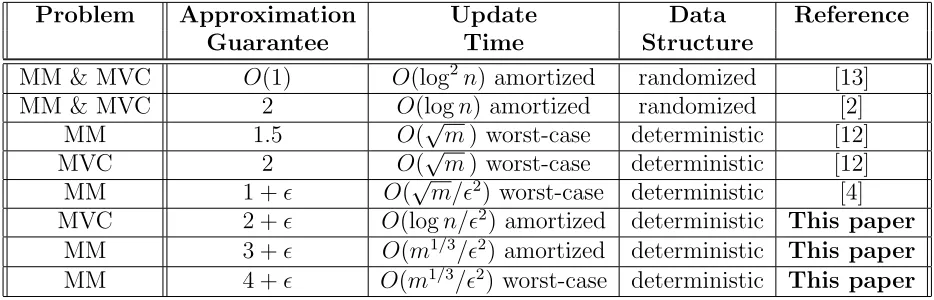
Table 1 puts our main results in perspective with previous work.
Our techniques. To see why it is difficult to determin-istically maintain a dynamic (say maximal) matching, consider the scenario when a matched edge incident to a nodeugets deleted from the graph. To recover from this deletion, we have to scan through the adjacency list of u to check if it has any free neighbor z. This takes time proportional to the degree of u, which can be O(n). Both the papers [2, 13] use randomization to circumvent this problem. Roughly speaking, the idea is to match the node u to one of its free neighbors z
pickedat random, and show that even if this step takes
O(deg(u)) time, in expectation the newly matched edge (u, z) survives the next deg(u)/2 edge deletions in the graph (assuming that the adversary is not aware of the random choices made by the data structure). This is used to bound the amortized update time.
Problem
Approximation
Update
Data
Reference
Guarantee
Time
Structure
MM & MVC
O
(1)
O
(log
2n
) amortized
randomized
[13]
MM & MVC
2
O
(log
n
) amortized
randomized
[2]
MM
1
.
5
O
(
√
m
) worst-case
deterministic
[12]
MVC
2
O
(
√
m
) worst-case
deterministic
[12]
MM
1 +
O
(
√
m/
2) worst-case
deterministic
[4]
MVC
2 +
O
(log
n/
2) amortized
deterministic
This paper
MM
3 +
O
(
m
1/3/
2) amortized
deterministic
This paper
[image:4.612.73.540.76.226.2]MM
4 +
O
(
m
1/3/
2) worst-case
deterministic
This paper
Table 1: Dynamic data structures for approximate (integral) maximum matching (MM) and minimum vertex cover (MVC).
the framework of Onak and Rubinfeld [13]. Roughly speaking, they maintain a hierarchical partition of the set of nodesV intoO(logn) levels such that the nodes in all but the lowest level, taken together, form a valid vertex cover V∗. In addition, they maintain a matching M∗ as a dual certificate. Specifically, they show that |V∗| ≤λ· |M∗| for some constant λ, which implies that V∗ is a λ-approximate minimum vertex cover. Their data structure is randomized since, as discussed above, it is particularly difficult to maintain the matchingM∗deterministically in a dynamic setting. To make the data structure deterministic, instead of
M∗, we maintain a fractional matching as a dual certificate. Along the way, we improve the amortized update time of [13] fromO(log2n) toO(logn/2), and
their approximation guarantee from some large constant
λto 2 +.
Our approach gives near-optimal bounds for fully dynamic minimum vertex cover and, as we have already remarked, it maintains a fractional matching. Next, we consider the problem of maintaining an approxi-mate maximumintegral matching, for which we are able to provide deterministic data structures with improved (polynomial) update time. Towards this end, we in-troduce the concept of a kernel of a graph, which we believe is of independent interest. Intuitively, a kernel is a subgraph with two important properties: (i) each node has bounded degree in the kernel, and (ii) a ker-nel approximately preserves the size of the maximum matching in the original graph. Our key contribution is to show that a kernel always exists, and that it can be maintained efficiently in a dynamic graph undergoing a sequence of edge updates.
2 Deterministic Fully Dynamic Vertex Cover
The input graphG= (V, E) has|V|=nnodes and zero edges in the beginning. Subsequently, it keeps getting updated due to the insertions of new edges and the deletions of already existing edges. The edge updates, however, occur one at a time, while the set V remains fixed. The goal is to maintain an approximate vertex cover ofGin this fully dynamic setting.
In Section 2.1, we introduce the notion of an (α, β )-partition of G= (V, E). This is a hierarchical partition of the setV intoL+1 levels, whereL=dlogβ(n/α)eand
α, β >1 are two parameters (Definition 1). If the (α, β )-partition satisfies an additional property (Invariant 1), then from it we can easily derive a 2αβ-approximation to the minimum vertex cover (Theorem 2.2). In Sec-tion 2.3, we present a natural deterministic algorithm for maintaining such an (α, β)-partition, and analyze it in Sections 2.5, 2.6 by settingα←1 + 2andβ ←1 +. Our main result is summarized in the theorem below.
Theorem 2.1. For every ∈(0,1], we can
determin-istically maintain a (2 +)-approximate vertex cover in a fully dynamic graph, the amortized update time being
O(logn/2).
2.1 The (α, β)-partition and its properties.
Definition 1. An (α, β)-partition of the graphG
par-titions its node-set V into subsetsV0. . . VL, whereL= dlogβ(n/α)eandα, β >1. For i∈ {0, . . . , L}, we iden-tify the subset Vi as the ith level of this partition, and
denote the level of a node v by `(v). Thus, we have
v ∈V`(v) for all v ∈V. Furthermore, the partition
as-signs a weight w(u, v) = β−max(`(u),`(v)) to every edge (u, v)∈V.
Given an (α, β)-partition, let Nv(i) ⊆ Nv denote the
set of neighbors of v that are in the ith level, and let Nv(i, j) ⊆ Nv denote the set of neighbors of v whose
levels are in the range [i, j].
(2.1) Nv ={u∈V : (u, v)∈E} ∀v∈V.
(2.2) Nv(i) ={u∈ Nv∩Vi} ∀v∈V;i∈ {0, . . . , L}
(2.3)
Nv(i, j) = j
[
k=i
Nv(k) ∀v∈V;i, j∈ {0, . . . , L}, i≤j.
Similarly, define the notations Dv and Dv(i, j).
Note thatDv is the degree of a nodev∈V.
(2.4) Dv=|Nv|
(2.5) Dv(i, j) =|Nv(i, j)|
Given an (α, β)-partition, letWv=Pu∈Nvw(u, v) denote the total weight a nodev∈V receives from the edges incident to it. We also define the notationWv(i).
It gives the total weight the nodev would receive from the edges incident to it, if the node v itself were to go to the ith level. Thus, we have W
v =Wv(`(v)). Since
the weight of an edge (u, v) in the hierarchical partition is given by w(u, v) = β−max(`(u),`(v)), we derive the
following equations for all nodesv∈V.
(2.6) Wv=
X
u∈Nv
β−max(`(u),`(v)).
(2.7) Wv(i) =
X
u∈Nv
β−max(`(u),i) ∀i∈ {0, . . . , L}.
Lemma 2.1. Every(α, β)-partition of the graph G
sat-isfies the following conditions for all nodes v∈V.
(2.8) Wv(L)≤α
(2.9) Wv(L)≤ · · · ≤Wv(i)≤ · · · ≤Wv(0)
(2.10) Wv(i)≤β·Wv(i+ 1) ∀i∈ {0, . . . , L−1}.
Proof. Fix any (α, β)-partition and any node v ∈ V. We prove the first part of the lemma as follows.
Wv(L) =
X
u∈Nv
β−max(`(u),L)
= X
u∈Nv
β−L≤n·β−L≤n·β−logβ(n/α)=α.
We now fix any level i ∈ {0, . . . , L−1} and show that the (α, β)-partition satisfies equation 2.9.
Wv(i+ 1) =
X
u∈Nv
β−max(`(u),i+1)
≤ X
u∈Nv
β−max(`(u),i)=Wv(i).
Finally, we prove equation 2.10.
Wv(i) =
X
u∈Nv
β−max(`(u),i)=β· X u∈Nv
β−1−max(`(u),i)
≤β· X
u∈Nv
β−max(`(u),i+1)=β·Wv(i+ 1)
Fix any node v ∈ V, and focus on the value of
Wv(i) as we go down from the highest leveli=Lto the
lowest level i = 0. Lemma 2.1 states that Wv(i) ≤ α
wheni=L, thatWv(i) keeps increasing as we go down
the levels one after another, and that Wv(i) increases
by at most a factor ofβ between consecutive levels. We will maintain a specific type of (α, β)-partition, where each node is assigned to a level in a way that satisfies Invariant 1.
Invariant 1. For every node v ∈V, if`(v) = 0, then
Wv≤α·β. Else if`(v)≥1, then Wv∈[1, αβ].
Consider any (α, β)-partition satisfying Invariant 1. Let v ∈ V be a node in this partition that is at level `(v) = k ∈ {0, . . . , L}. It follows that P
u∈Nv(0,k)w(u, v) = |Nv(0, k)| ·β
−k ≤ W
v ≤ αβ.
Thus, we infer that|Nv(0, k)| ≤αβk+1. In other words,
Invariant 1 gives an upper bound on the number of neighbors a node v can have that lie on or below `(v). We will crucially use this property in the analysis of our algorithm.
Theorem 2.2. Consider an (α, β)-partition of the
graph G that satisfies Invariant 1. Let V∗ ={v ∈V :
Wv ≥ 1} be the set of nodes with weight at least one.
The set V∗ is a feasible vertex cover inG. Further, the
size of the set V∗ is at most 2αβ-times the size of the minimum-cardinality vertex cover in G.
Proof. Consider any edge (u, v) ∈ E. We claim that at least one of its endpoints belong to the set V∗. Suppose that the claim is false and we have Wu < 1
andWv<1. If this is the case, then Invariant 1 implies
that`(u) =`(v) = 0 andw(u, v) =β−max(`(u),`(v))= 1. Since Wu ≥w(u, v) and Wv ≥w(u, v), we get Wu ≥1
and Wv ≥ 1, and this leads to a contradiction. Thus,
Next, we construct a fractional matching Mf by
picking every edge (u, v)∈E to an extent ofx(u, v) =
w(u, v)/(αβ)∈[0,1]. Since for all nodesv∈V, we have P
u∈Nvx(u, v) = P
u∈Nvw(u, v)/(αβ) =Wv/(αβ)≤1, we infer that Mf is a valid fractional matching in
G. The size of this matching is given by |Mf| =
P
(u,v)∈Ex(u, v) = (1/(αβ))·
P
(u,v)∈Ew(u, v). We now
bound the size ofV∗ in terms of|M
f|.
|V∗|= X
v∈V∗
1≤ X v∈V∗
Wv=
X
v∈V∗
X
u∈Nv
w(u, v)
≤X
v∈V
X
u∈Nv
w(u, v) = 2· X
(u,v)∈E
w(u, v) = (2αβ)· |Mf|
2.2 Query time. We store the nodes v with Wv ≥
1 as a separate list. Thus, we can report the set of nodes in the vertex cover in O(1) time per node. Using appropriate pointers, we can report inO(1) time whether or not a given node is part of this vertex cover. In O(1) time we can also report the size of the vertex cover.
2.3 Handling the insertion/deletion of an edge. A node is calleddirtyif it violates Invariant 1, andclean otherwise. Since the graphG= (V, E) is initially empty, every node is clean and at level zero before the first update in G. Now consider the time instant just prior to thetthupdate inG. By induction hypothesis, at this
instant every node is clean. Then the tth update takes
place, which inserts (resp. deletes) an edge (x, y) in G
with weight w(x, y) = β−max(`(x),`(y)). This increases
(resp. decreases) the weights Wx, Wy byw(x, y). Due
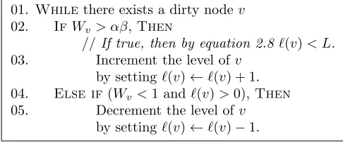
to this change, the nodes xandy might become dirty. To recover from this, we call the subroutine in Figure 1.
01. Whilethere exists a dirty nodev
02. IfWv> αβ,Then
//If true, then by equation 2.8 `(v)< L. 03. Increment the level of v
by setting`(v)←`(v) + 1. 04. Else if(Wv<1 and`(v)>0),Then
05. Decrement the level ofv
[image:6.612.59.302.500.604.2]by setting`(v)←`(v)−1.
Figure 1: RECOVER().
Consider any node v ∈ V and suppose that Wv =
Wv(`(v))> αβ. In this event, equation 2.8 implies that
Wv(L) < Wv(`(v)) and hence we have L > `(v). In
other words, when the procedure described in Figure 1 decides to increment the level of a dirty node v (Step 02), we know for sure that the current level of v is strictly less than L (the highest level in the (α, β
)-partition).
Next, consider a node z ∈ Nv. If we change
`(v), then this may change the weightw(v, z), and this in turn may change the weight Wz. Thus, a single
iteration of the While loop in Figure 1 may lead to some clean nodes becoming dirty, and some other dirty nodes becoming clean. If and when the While loop terminates, however, we are guaranteed that every node is clean and that Invariant 1 holds.
Comparison with the framework of Onak and Rubinfeld [13]. As described below, there are two significant differences between our framework and that of [13]. Consequently, many of the technical details of our approach (illustrated in Section 2.6) differ from the proof in [13].
First, in the hierarchical partition of [13], the invariant for a node y consists ofO(L) constraints: for each level i∈ {`(y), . . . , L}, the quantity |Ny(0, i)| has
to lie within a certain range. This is the main reason for their amortized update time being Θ(log2n). Indeed when a nodeybecomes dirty, unlike in our setting, they have to spend Θ(logn) time just to figure out the new level ofy.
Second, along with the hierarchical partition, the authors in [13] maintain a matching as adual certificate, and show that the size of this matching is within a constant factor of the size of their vertex cover. As pointed out in Section 1, this is the part where they crucially need to use randomization, as till date there is no deterministic data structure for maintaining a large matching in polylog amortized update time. We bypass this barrier by implicitly maintaining afractional matching as a dual certificate. Indeed, the weight
w(y, z) of an edge (y, z) in our hierarchical partition, after suitable scaling, equals the fractional extent by which the edge (y, z) is included in our fractional matching.
2.4 Data structures. We now describe the relevant data structures that will be used to implement our algorithm.
• We maintain for each nodev∈V:
– A counter Level[v] to keep track of the current level of v. Thus, we setLevel[v] ←
`(v).
– A counter Weight[v] to keep track of the weight of v. Thus, we setWeight[v]←Wv.
– For every leveli >Level[v], the set of nodes
Nv(i) in the form of a doubly linked list
Neighborsv[i]. For every leveli≤Level[v],
– For level i = Level[v], the set of nodes
Nv(0, i) in the form of a doubly linked
list Neighborsv[0, i]. For every level i 6=
Level[v], the listNeighborsv[0, i] is empty. • When the graph G gets updated due to an edge insertion/deletion, we may discover that a node violates Invariant 1. Such a node is calleddirty, and we store the set of such nodes as a doubly linked list
Dirty-nodes. For every nodev∈V, we maintain
a bit Status[v] ∈ {dirty,clean} that indicates if the node is dirty or not. Every dirty node stores a pointer to its position in the listDirty-nodes.
• We use the phrase “neighborhood lists of
v” to refer to the collection of linked lists
SL
i=0{Neighborsv[0, i],Neighborsv[i]}. For
every edge (u, v), we maintain two bidirectional pointers: one links the edge to the position ofv in the neighborhood lists of u, while the other links the edge to the position of uin the neighborhood lists ofv. Using these pointers, we can update the neighborhood lists ofuandv when the edge (u, v) is inserted into (resp. deleted from) the graph, or when the node v increases (resp. decreases) its level by one.
2.5 Bounding the amortized update time. In the full version of this paper, we present a detailed implementation of our algorithm using the data struc-tures described in Section 2.4. We also prove that for any ∈ [0,1], α = 1 + 2 and β = 1 +, it takes
O(tlogn/2) time to handletedge insertions/deletions
inGstarting from an empty graph. This gives an amor-tized update time ofO(logn/2), and by Theorem 2.2,
a (2 + 10)-approximation to the minimum vertex cover in G. Specifically we show that after an edge insertion or deletion the data structure can be updated in time
O(1) plus the time to adjust the levels of the nodes, i.e., the time for procedure RECOVER. To bound the latter we show that it takes time Θ(1 +Dv(0, i)), when node
v changes from level i to level i+ 1 or level i−1 and prove the bound on the total time spent in procedure RECOVER using a potential function based argument. Due to space constraints, we give a (slightly) simpli-fied variant of this argument here, which gives an amor-tized bound onthe number of times we have to change the weight of an already existing edge. This number is
Dv(0, i), when nodev changes from levelito leveli+ 1
and Dv(0, i−1), when node v changes from level i to
level i−1.1 Specifically, we prove Theorem 2.3 in
Sec-1The proof actually shows a stronger result assuming that the
level change of node vfromi to i−1 causes Θ(Dv(0, i)) many
tion 2.6, which implies that on average we change the weights ofO(L/) =O(logn/2) edges per update inG.
Theorem 2.3. Set α ← 1 + 2, β ← 1 + . In
the beginning, when G is an empty graph, initialize a counter Count ← 0. Subsequently, each time we change the weight of an already existing edge in the hierarchical partition, setCount←Count+ 1. Then
Count =O(tL/) just after we handle the tth update
in G.
The proof in Section 2.6 uses a carefully chosen potential function. As the formal analysis is quite involved, some high level intuitions are in order. Below, we give a brief overview of our approach. To highlight the main ideas, in contrast with Theorem 2.3, we assume that αandβ are some sufficiently large constants.
Define the level of an edge (y, z) to be `(y, z) = max(`(y), `(z)), and note that the weight w(y, z) de-creases (resp. inde-creases) iff the edge’s level`(y, z) goes up (resp. down). There is a potential associated with both nodes and edges. Note that we use the terms “to-kens” and “potential” interchangeably.
Each edgee has exactly 2(L−`(e)) tokens. These tokens are assigned as follows. Whenever a new edge is inserted, it receives 2(L −`(e)) tokens. When e
moves up a level, it gives one token to each endpoint. Whenever e is deleted, it gives one token to each endpoint. Whenevere moves down a level because one endpoint, say u, moves down a level, e receives two tokens fromu.
Initially and whenever a node moves a level higher, it has no tokens. Whenever a node umoves up a level, only its adjacent edges to the same or lower levels have to be updated as their level changes. The level of all other edges is unchanged. Recall that each such edge gives 1 token tou, which in turn uses this token to pay for updating the edge. Whenever a node umoves down a level, say fromk tok−1, it has at mostβk adjacent
edges at levelkor below. These are all the edges whose level needs to be updated (which costs a token) and whose potential needs to be increased by two tokens. In this case we show that u has enough tokens, (i) to pay for the work involved in the update, (ii) to give two tokens to each of the at most βk adjacent edges, and
(iii) to still have a sufficient number of tokens for being on levelk−1.
Whenever the level of a node v is not modified but its weight Wv decreases because the weight of the
adjacent edge (u, v) decreases, the level of (u, v) must have increased and (u, v) gives one token tov(the other one goes tou). Note that this implies that a change in
Wv by at mostβ−`(v)increases the potential ofv by 1,
i.e., the “conversion rate” between weight changes and token changes isβ`(v). Whenever the level ofvdoes not
change but its weight Wv increasesas the level of (u, v)
has decreased, no tokens are transferred betweenvand (u, v). (Technically the potential ofvmight fall slightly but the change might be so small that we ignore it.) Formally we achieve these potential function changes by setting the potential of every node inV0to 0 and for
every other node toβ`(v)·max(0, α−W
v).
Thus, the crucial claim is that a nodev that moves down to levelk−1 has accumulated a sufficent number of tokens, i.e., at leastX := 3βk+βk−1max(0, α−W
v(k−
1)) tokens. Case 1: Assume first thatv’s immediately preceeding level was on levelk−1, i.e. thatv just had moved up from levelk−1. Recall that, by the definition of the potential function,vhadnotokens when it moved up from levelk−1. However, in this case we know that
Wv was leastαβand, thus, after adjusting the weight of
its adjacent edges to the level change,Wvis still at least
αafter the level change. Nodevonly drops to levelk−1 if Wv <1, i.e., while being on level k its weight must
have dropped by at leastα−1. By the above “conversion rate” between weight and tokens this means thatvmust have received at least βk(α−1) tokens while it was on
level k, which at leastX for large enough α. Case 2: Assume next that nodevwas at levelk+ 1 immediately before levelk. Right after dropping from levelk+1 node
v ownedβk(α−W
v(k)) tokens. As v has not changed
levels since, it did not have to give any tokens to edges and did not have to pay for any updates of its adjacent edges. Instead it might have received some tokens from inserted or deleted adjacent edges. Thus, it still ownes at least βk(α−W
v(k)) tokens. AsWv(k)≤Wv(k−1)
andWv(k)<1 whenvdrops to levelk−1, this number
of tokens is at leastX forβ≥2 andα≥3β+ 1. To summarize, whenever an edge is inserted it receives a sufficient number of tokens to pay the cost of future upwards level changes, but also to give a token to its “lower” endpoint every time its level increases. These tokens accumulated at the “lower” endpoints are sufficient to pay for level decreases of these endpoints because (a) nodes move up to a level when their weight on the new level is at leastα >1 but only move down when their weight falls below 1 and (b) the weight of edges on the same and lower levels drops by a factor of
β between two adjacent levels. Thusβk(α−1) many
edge deletions or edge weight decreases of edges adjacent to node vare necessary to cause v to drop from levelk
to levelk−1 (each giving one token to v), while there are only βk−1 many edges on levels below k that need to be updated whenv drops. Thus, the cost ofv’s level drop is βk−1 and the new potential needed for v on
level k−1 is βk−1(α−1), butv has collected at least
βk(α−1) tokens, which, by suitable choice of β andα,
is sufficient.
2.6 Proof of Theorem 2.3. Recall that the level of an edge (y, z) is defined as `(y, z) = max(`(y), `(z)). Consider the following thought experiment. We have a bank account, and initially, when there are no edges in the graph, the bank account has zero balance. For each subsequent edge insertion/deletion, at mostL/dollars are deposited to the bank account; and every time our algorithm changes the level of an already existing edge, 1 dollar is withdrawn from it. We show that the bank account never runs out of money, and this implies
thatCount=O(tL/) aftertedge insertions/deletions
starting from an empty graph.
LetBdenote the total amount of money (or poten-tial) in the bank account at the present moment. We keep track ofBby distributing an-fraction of it among the nodes and the current set of edges in the graph.
(2.11) B= (1/)· X e∈E
Φ(e) +X
v∈V
Ψ(v) !
In the above equation, the amount of money (or potential) associated with an edge e ∈ E is given by Φ(e), and the amount of money (or potential) associated with a node v ∈ V is given by Ψ(v). To ease notation, for each edge e = (u, v) ∈ E, we use the symbols Φ(e),Φ(u, v) and Φ(v, u) interchangeably. At every point in time, all the potentials Φ(u, v),Ψ(v) are determined by the two invariants stated below.
Invariant 2. For every edge (u, v)∈E, we have:
Φ(u, v) = (1 +)·(L−max(`(u), `(v)))
Invariant 3. For every node v∈V, we have:
Ψ(v) =β`(v)+1/(β−1)·max (0, α−Wv)
When the algorithm starts, the graph has zero edges, all the nodes are at level 0, and every node is passive. At that moment, Invariant 3 sets Ψ(v) = 0 for all nodes v ∈ V. Consequently, equation 2.11 implies that the potentialBis also set to zero. This is consistent with our requirement that initially the bank account ought to have zero balance. Theorem 2.3, therefore, will follow if we can prove the next two lemmas. Their proofs appear in Section 2.6.1 and Section 2.6.2 respectively.
Lemma 2.2. Consider the insertion (resp. deletion)
destroys) the potential Φ(u, v), and increases (resp. decreases) the potentialΨ(u)(resp. Ψ(v)). Due to these changes, the total potentialB increases by at mostL/.
Lemma 2.3. During every single iteration of the
While loop in Figure 1, the total increase in Count
is no more than the net decrease in the potentialB.
2.6.1 Proof of Lemma 2.2. If an edge (u, v) is inserted intoG, then the potential Φ(u, v) is created and gets a value of at most (1 +)Lunits. As the weightWu
(resp. Wv) increases, it follows that the potential Ψ(u)
(resp. Ψ(v)) does not increase. All the other potentials remain unchanged. Thus, the net increase in B is at most (1/)·(1 +)L= (1 + 1/)L≤L/.
In contrast, if an edge (u, v) is deleted from G, then the potential Φ(u, v) is destroyed. The weight Wu
(resp. Wv) decreases by at most β−`(u) (resp. β−`(v)).
Hence, each of the potentials Ψ(u),Ψ(v) increases by at most β/(β−1) = 1 + 1/ ≤ (1 +)/log(1 +) ≤
((logn)−1)/log(1 +)≤Lforn≥8. The potentials of the remaining nodes and edges do not change. Hence, by equation 2.11, the net increase inB is at mostL/.
2.6.2 Proof of Lemma 2.3.
Throughout this section, fix a single iteration of the
While loop in Figure 1 and suppose that it changes
the level of a dirty node v by one unit. We use the superscript 0 (resp. 1) on a symbol to denote its state at the time instant immediately prior to (resp. after) that specific iteration of the Whileloop. Further, we preface a symbol withδto denote the net decrease in its value due to that iteration. For example, consider the potential B. We have B = B0 immediately before the
iteration begins, andB=B1immediately after iteration
ends. We also haveδB=B0− B1.
A change in the level of node v affects only the potentials of the nodes u ∈ Nv∪ {v} and that of the
edges e∈ {(u, v) :u∈ Nv}. This observation, coupled
with equation 2.11, gives us the following guarantee.
(2.12)
δB= (1/)· δΨ(v) + X
u∈Nv
δΦ(u, v) + X
u∈Nv
δΨ(u) !
A change in the level of nodev does not affect the (a) the neighborhood structure of the node v, and (b) the level and the overall degree of any nodeu6=v. Thus, we get the following equalities.
N0
v(i) = Nv1(i) for alli∈ {0, . . . , L}.
(2.13)
`0(u) = `1(u) for allu∈V \ {v}.
(2.14)
D0u = D
1
u for allu∈V \ {v}.
(2.15)
Accordingly, to ease notation we do not put any superscript on the following symbols, as the quantities they refer to remain the same throughout the duration of the iteration of the While loop we are concerned about.
Nv, Dv.
Nv(i), Wv(i) for alli∈ {0, . . . , L}.
Nv(i, j),Dv(i, j) for alli, j∈ {0, . . . , L}, i≤j.
`(u), Du for allu∈V \ {v}.
We divide the proof of Lemma 2.3 into two possible cases, depending upon whether the concerned iteration of theWhileloop increments or decrements the level of
v. The main approach to the proof remains the same in each case. We first give an upper bound on the increase
in Count due to the iteration. Next, we separately
lower bound each of the following quantities: δΨ(v),
δΦ(u, v) for all u ∈ Nv, and δΨ(u) for all u ∈ Nv.
Finally, applying equation 2.12, we derive that δB is sufficiently large to pay for the increase inCount.
Case 1: The level of the nodev increases fromk
to (k+ 1).
Claim 1. We haveCount1−Count0=Dv(0, k).
Proof. When the node v changes its level from k to (k+ 1), this only affects the levels of those edges that are of the form (u, v), whereu∈ Nv(0, k).
Claim 2. We haveδΨ(v) = 0.
Proof. Since the node v increases its level from k to (k + 1), Step 02 (Figure 1) guarantees that W0
v =
Wv(k) > αβ. Next, from Lemma 2.1 we infer that
Wv1 = Wv(k+ 1) ≥ β−1· Wv(k) > α. Since both
Wv0, Wv1 > α, we get: Ψ0(v) = Ψ1(v) = 0. It follows
that δΨ(v) = Ψ0(v)−Ψ1(v) = 0.
Claim 3. For every nodeu∈ Nv, we have:
δΦ(u, v) = (
(1 +) if u∈ Nv(0, k);
0 if u∈ Nv(k+ 1, L).
Proof. Ifu∈ Nv(0, k), then we have Φ0(u, v) = (1 +)·
(L−k) and Φ1(u, v) = (1 +)·(L−k−1). It follows
that δΦ(u, v) = Φ0(u, v)−Φ1(u, v) = (1 +).
In contrast, if u ∈ Nv(k+ 1, L), then we have
Φ0(u, v) = Φ1(u, v) = (1 +)·(L−`(u)). Hence, we getδΦ(u, v) = Φ0(u, v)−Φ1(u, v) = 0.
Claim 4. For every nodeu∈ Nv, we have:
δΨ(u)≥
(
−1 if u∈ Nv(0, k);
Proof. Consider any node u ∈ Nv(k+ 1, L). Since
k < `(u), we havew0(u, v) =w1(u, v), and this implies
that W0
u =Wu1. Thus, we getδΨ(u) = 0.
Next, fix any nodeu∈ Nv(0, k). Note thatδWu=
δw(u, v) = β−k−β−(k+1) = (β −1)/βk+1. Using this observation, we infer that:
δΨ(u)≥ −β`(u)+1/(β−1)·δWu
=−β`(u)+1/βk+1≥ −1.
From Claims 2, 3, 4 and equation 2.12, we derive the following bound.
δB = (1/)· δΨ(v) + X
u∈Nv
δΦ(u, v) + X
u∈Nv
δΨ(u) !
≥ (1/)·(0 + (1 +)·Dv(0, k)−Dv(0, k))
= Dv(0, k)
Thus, Claim 1 implies that the net decrease in the potentialBin no less than the increase inCount. This proves Lemma 2.3.
Case 2: The level of the node v decreases from
k to k−1.
Claim 5. We haveWv0=Wv(k)<1,Dv(0, k)≤βk.
Proof. Since the node v decreases its level from k to (k−1), Step 04 (Figure 1) ensures thatW0
v =Wv(k)<
1. Since `0(v) = k, we have w0(u, v) ≥ β−k for all
u∈ Nv. We conclude that:
1> Wv0≥ X u∈Nv(0,k)
w0(u, v)≥β−k·Dv(0, k).
Thus, we getDv(0, k)≤βk.
Claim 6. We haveCount1−Count0≤βk.
Proof. The node v decreases its level from k to k−1. Due to this event, the level of an edge changes iff it is of the form (u, v) withu∈ Nv(0, k−1). Thus, we have
Count1−Count0=Dv(0, k−1)≤Dv(0, k)≤βk.
Claim 7. For allu∈ Nv, we have δΨ(u)≥0.
Proof. Fix any node u∈ Nv. As the level of the node
v decreases from k to k−1, we infer that w0(u, v) ≤
w1(u, v), and, accordingly, we get W0
u ≤ Wu1. Since
Ψ(u) =β`(u)·max (0, α−W
u), we derive that Ψ0(u)≥
Ψ1(u). Thus, we haveδΨ(u) = Ψ0(u)−Ψ1(u)≥0.
Claim 8. For every nodeu∈ Nv, we have:
δΦ(u, v) = (
0 if u∈ Nv(k, L); −(1 +) if u∈ Nv(0, k−1);
Proof. Fix any node u∈ Nv. We consider two possible
scenarios.
1. We have u∈ Nv(k, L). As the level of the node v
decreases fromkto k−1, we infer that Φ0(u, v) = Φ1(u, v) = (1 +)· (L−`(u)). Hence, we get
δΦ(u, v) = Φ1(u, v)−Φ0(u, v) = 0.
2. We haveu∈ Nv(0, k−1). Since the level of nodev
decreases fromkto k−1, we infer that Φ0(u, v) =
(1 +)·(L−k) and Φ1(u, v) = (1 +)·(L−k+ 1).
Hence, we get δΦ(u, v) = Φ1(u, v)−Φ0(u, v) =
−(1 +).
This concludes the proof of the claim.
We now partition W0
v into two parts: x and y.
The first part denotes the contributions towards W0
v
by the neighbors of v that lie below levelk, while the second part denotes the contribution towardsWv0by the neighbors of v that lie on or above level k. Note that
x=P
u∈Nv(0,k−1)w
0(u, v) =β−k·D
v(0, k−1). Thus,
we get the following equations.
Wv0=x+y≤1 (2.16)
x=β−k·Dv(0, k−1)
(2.17)
y= X
u∈Nv(k,L)
w0(u, v) (2.18)
Equation 2.16 holds due to Claim 5.
Claim 9. We haveP
u∈NvδΦ(u, v) =−(1 +)·x·β
k.
Proof. Claim 8 implies that P
u∈NvδΦ(u, v) = −(1 +
)·Dv(0, k−1). Applying equation 2.17, we infer that
Dv(0, k−1) =x·βk.
Claim 10. We have:
δΨ(v) = (α−x−y)· βk+1/(β−1)
−max (0, α−βx−y)· βk/(β−1).
Proof. Equation 2.16 states thatWv0=x+y <1. Since
`0(v) =k, we get:
(2.19) Ψ0(v) = (α−x−y)· βk+1/(β−1) As the node v decreases its level from k to k−1, we have:
w1(u, v) = (
β·w0(u, v) ifu∈ N
v(0, k−1);
w0(u, v) ifu∈ N
v(k, L)
Accordingly, we haveW1
v =β·x+y, which implies the
following equation.
We now consider two possible scenarios depending upon the value of (α−βx−y). We show that in each case δB ≥βk. This, along with Claim 6, implies that
δB ≥Count1−Count0. This proves Lemma 2.3.
1. Suppose that (α−βx−y)<0. From Claims 7, 9, 10 and equation 2.12, we derive:
·δB = X
u∈Nv
δΨ(u) + X
u∈Nv
δΦ(u, v) + Ψ(v)
≥ −(1 +)·x·βk+ (α−x−y)· β k+1
(β−1)
≥ −(1 +)·βk+ (α−1)·βk+1/(β−1)
= β
k
(β−1) · {(α−1)·β−(1 +)(β−1)} = (1 +)·βk
≥ ·βk
The last equality holds since α = 1 + 2 and
β = 1 +.
2. Suppose that (α−βx−y)≥0. From Claims 7, 9, 10 and equation 2.12, we derive:
·δB = X
u∈Nv
δΨ(u) + X
u∈Nv
δΦ(u, v) + Ψ(v)
≥ −(1 +)·x·βk+ (α−x−y)· β k+1
(β−1)
−(α−βx−y)·βk/(β−1)
= β
k
(β−1) ·
(α−x−y)·β
−(1 +)·x·(β−1)−(α−βx−y)
= β
k
(β−1) ·
(α−x−y)·(β−1)
−·x·(β−1)
≥ β
k
(β−1) ·
(α−1)(β−1)−(β−1)
= ·βk (since α= 1 + 2, β= 1 +)
3 Dynamic Matching: Preliminaries
We are given an input graph G= (V, E) that is being updated dynamically through a sequence of edge inser-tions/deletions. We want to maintain an approximately maximum matching inG. We will present two different algorithms for this problem. They are described in Sec-tions 4 and 5. Both these algorithms, however, will use two key ideas.
1. It is easy to maintain a good approximate matching in a bounded degree graph (see Section 3.1).
2. Every graph contains a subgraph of bounded de-gree, called itskernel, that approximately preserves the size of the maximum matching (see Section 3.2).
In Section 3.3, we give a static algorithm for building a kernel in a graph. In Section 3.4, we present the data structures that will be used in Sections 4 and 5 for maintaining a kernel in a dynamic setting.
Query time. In this paper, all the data structures for dynamic matching explicitly maintain the set of matched edges. Accordingly, using appropriate point-ers, we can support the following queries.
• Report the size of the matchingM maintained by the data structure in O(1) time.
• Report the edges inM inO(1) time per edge.
• In O(1) time, report whether or not a given edge (u, v) is part of the matching.
• In O(1) time, report whether or not a given node
uis matched inM, and if yes, inO(1) time report the node it is matched to.
3.1 Maintaining an approximate matching in a bounded degree graph.
Maintaining a maximalmatching in a graph with max-imum degree δ in time O(δ) per deletion and O(1) per edge insertion is straightforward: After an inser-tion check whether the inserted edge can be added to the matching. If a matched edge is deleted, check all neighbors of its endpoints to rematch them if possible. Following the approach from [12], we can show that in
O(δ) worst-case update time we can even maintain a 3/2-approximatematching by guaranteeing that no aug-menting path has a length less than 5. The basic idea is to keep for each node a list of its neighbors as well as a list of its unmatched neighbors. Due to space con-straints, the proofs of the next two theorems appear in the full version of the paper.
Theorem 3.1. Consider a dynamic graphG = (V,E),
and suppose that the maximum degree of a node in
G is always upper bounded by δ. There exists a data structure for maintaining a maximal matching M in G
that handles each edge insertion in O(1)time and each edge deletion in O(δ)time.
Theorem 3.2. Consider a dynamic graphG = (V,E),
3.2 The kernel and its properties.
In the input graph G = (V, E), let Nv = {u ∈ V :
(u, v)∈E} denote the set ofneighborsofv∈V. Consider a subgraphκ(G) = (V, κ(E)) withκ(E)⊆
E. For all v ∈ V, define the set κ(Nv) = {u ∈ Nv :
(u, v) ∈ κ(E)}. If u ∈ κ(Nv), then we say that u
is a friend of v in κ(G). Next, the set of nodes V
is partitioned into two groups: tight and slack. We denote the set of tight (resp. slack) nodes by κT(V)
(resp.κS(V)). Thus, we haveV =κT(V)∪κS(V) and
κT(V)∩κS(V) =∅.
Definition 2. Fix anyc≥1and any∈[0,1/3). The
subgraphκ(G)is an(, c)-kernel ofGwith respect to the partition (κT(V), κS(V))iff it satisfies Invariants 4- 6.
Invariant 4. |κ(Nv)| ≤ (1 +)c for all v ∈ V, i.e.,
every node has at most (1 +)c friends.
Invariant 5. |κ(Nv)| ≥ (1−)c for all v ∈ κT(V),
i.e., every tight node has at least (1−)c friends.
Invariant 6. For all u, v ∈κS(V), if (u, v)∈E, then
(u, v) ∈ κ(E). In other words, if two slack nodes are connected by an edge in G, then that edge must belong toκ(G).
By Invariant 4, the maximum degree of a node in an (, c)-kernel is O(c). In Theorems 3.3 and 3.4, we show that an (, c)-kernel κ(G) is basically a subgraph of G with maximum degree O(c) that approximately preserves the size of the maximum matching.
For ease of exposition, we often refer to a kernel
κ(G) without explicitly mentioning the underlying par-tition (κT(V), κS(V)). The proofs of Theorems 3.3, 3.4
appear in Sections 3.2.1 and 3.2.2 respectively.
Theorem 3.3. Let M be a maximal matching in an
(, c)-kernel κ(G). ThenM is a(4 + 6)-approximation to the maximum matching in G.
Theorem 3.4. Let M be a matching in an (, c)
-kernel κ(G) such that every augmenting path in κ(G) (w.r.t.M) has length at least five. ThenM is a(3+3) -approximation to the maximum matching in G.
3.2.1 Proof of Theorem 3.3.
Let V(M) = {v ∈ V : (u, v) ∈ M for some u ∈ Nv}
be the set of nodes that are matched in M, and let
FT = κT(V)\V(M) be the subset of tight nodes in
κ(G) that are free in M.
Lemma 3.1. We have|FT| ≤(2 + 6)· |M|.
Proof. We will show that|FT| ≤(1 + 3)·|V(M)|. Since |V(M)|= 2· |M|, the lemma follows.
We design a charging scheme where each node in
FT contributes one dollar to a global fund. So the
total amount of money in this fund is equal to |FT|
dollars. Below, we demonstrate how to transfer this fund to the nodes inV(M) so that each nodex∈V(M) receives at most (1 + 3) dollars. This implies that
|FT| ≤(1 + 3)· |V(M)|.
Since M is a maximal matching in κ(G), we must have κ(Nv) ⊆ V(M) for all v ∈ FT. For each node
v ∈ FT, we distribute its one dollar equally among
its friends, i.e., each node x ∈ κ(Nv) gets 1/|κ(Nv)|
dollars from v. Since FT ⊆κT(V), Invariant 5 implies
that 1/|κ(Nv)| ≤1/((1−)c) for all v∈ FT. In other
words, a node in V(M) receives at most 1/((1−)c) dollars from each of its friends under this money-transfer scheme. But, by Invariant 4, a node can have at most (1 + )c friends. So the total amount of money received by a node in V(M) is at most (1 +)c/((1−)c)≤(1 + 3), for∈[0,1/3).
To continue with the proof of Theorem 3.3, let
Mo ⊆ E be a maximum-cardinality matching in G = (V, E). Define M1o ⊆ Mo to be the subset of edges
whose both endpoints are unmatched in M, and let
Mo
2 =Mo\M1o.
Consider any edge (u, v)∈Mo
1. By definition, both
the nodes u, v are free in M. Since M is a maximal matching in κ(G), it follows that the edge (u, v) is not part of the kernel, i.e., (u, v)6=κ(E). Hence, Invariant 6 implies that either u /∈κS(V) or v /∈κS(V). Without
any loss of generality, suppose that u /∈ κS(V). This
means that the node uis tight, and, furthermore, it is free in M. We infer that every edge in Mo
1 is incident
to at least one node fromFT, whereFT ⊆κT(V) is the
subset of tight nodes that are free in M. Accordingly, we have |M1o| ≤ |FT|. Combining this inequality with
Lemma 3.1, we get:
(3.21) |M1o| ≤(2 + 6)· |M|
Next, every edge in Mo
2 has at least one endpoint
that is matched inM. Thus,M is a maximal matching in the graph G0 = (V, Mo
2 ∪M). Since M2o is also a
matching inG0, we get:
(3.22) |M2o| ≤2· |M|
The theorem follows if we add equations 3.21 and 3.22.
3.2.2 Proof of Theorem 3.4.
Let V(M) = {v ∈ V : (u, v) ∈ M for some u ∈ Nv}
be the set of nodes that are matched in M. For all nodes v∈V(M), leteM(v) denote the edge in M that
is incident tov. LetFT =κT(V)\V(M) be the subset
Lemma 3.2. For every edge (u, v) ∈ M, we have
|(κ(Nu)∩FT)∪(κ(Nv)∩FT)| ≤(1 +)c.
Proof. Suppose that the lemma is false and we have
|(κ(Nu)∩FT)∪(κ(Nv)∩FT)|>(1 +)cfor some edge
(u, v)∈ M. As Invariant 4 guarantees that |κ(Nu)| ≤
(1 +)c and |κ(Nv)| ≤(1 +)c, there has to be a pair
of distinct nodes u0, v0 ∈FT such thatu0 ∈κ(Nu) and
v0 ∈ κ(Nv). This means that the path (u0, u, v, v0) is
an augmenting path inκ(G) (w.r.t.M) and has length three. We reach a contradiction.
Lemma 3.3. We have|FT| ≤(1 + 3)· |M|.
Proof. We design a charging scheme where each node in
FT contributes one dollar to a global fund. So the total
amount of money in this fund is equal to |FT| dollars.
Below, we demonstrate how to transfer this fund to the edges in M so that each edge e∈ M receives at most (1 + 3) dollars. This implies that|FT| ≤(1 + 3)· |M|.
Since M is a maximal matching in κ(G), we must have κ(Nv) ⊆ V(M) for all v ∈ FT. For each node
v ∈ FT, we distribute its one dollar equally among
the matched edges incident to its friends, i.e., for each node x∈κ(Nv), the edgeeM(x) gets 1/|κ(Nv)|dollars
from v. Since FT ⊆ κT(V), Invariant 5 implies that
1/|κ(Nv)| ≤1/((1−)c) for allv∈FT. In other words,
an edge (x, y)∈M receives at most 1/((1−)c) dollars from each of the nodesv∈(κ(Nx)∩FT)∪(κ(Ny)∩FT)
under this money-transfer scheme. Hence, Lemma 3.2 implies that the total amount of money received by an edge (x, y)∈M is at most (1 +)c/((1−)c)≤(1 + 3), for∈[0,1/3).
To continue with the proof of Theorem 3.4, define
Mo ⊆ E to be a maximum-cardinality matching in
G= (V, E). Furthermore, let M1o⊆Mo be the subset of edges whose both endpoints are unmatched in M, and letM2o=Mo\M1o.
Consider any edge (u, v)∈Mo
1. By definition, both
the nodes u, v are free in M. Since M is a maximal matching in κ(G), it follows that the edge (u, v) is not part of the kernel, i.e., (u, v) 6= κ(E). Hence, Invariant 6 implies that eitheru /∈κS(V) orv /∈κS(V).
Without any loss of generality, suppose thatu /∈κS(V).
This means that the node uis tight, and, furthermore, it is free in M. We infer that every edge in Mo
1 is
incident to at least one node from FT. Accordingly,
we have |Mo
1| ≤ |FT|. Combining this inequality with
Lemma 3.3, we get:
(3.23) |M1o| ≤(1 + 3)· |M|
Next, every edge in M2o has at least one endpoint
that is matched inM. Thus,M is a maximal matching
in the graph G0 = (V, Mo
2 ∪M). Since M2o is also a
matching inG0, we get:
(3.24) |M2o| ≤2· |M|
The theorem follows if we add equations 3.23 and 3.24.
3.3 An algorithm for building a kernel in a static graph.
We present a linear-time algorithm for constructing a (0, c)-kernelκ(G) of a static graphG= (V, E).
Theorem 3.5. We have an algorithm for computing a
(0, c)-kernel κ(G) = (V, κ(E)) of a graph G= (V, E). The kernel returned by the algorithm has the added property that tight nodes have exactlycfriends and slack nodes have less than c friends. For every c ≥ 1, the algorithm runs in O(|E|)time.
Proof. Initially, each node in V has zero friends, and the edge-set κ(E) is empty. We then execute the For loop stated below.
• For all(u, v)∈E
– if|κ(Nu)|< c and|κ(Nv)|< c,Then ∗ Set κ(Nv) ←κ(Nv)∪ {u} and κ(Nu) ←
κ(Nu)∪ {v}.
∗ Setκ(E)←κ(E)∪ {(u, v)}.
Consider theκ(G) = (V, κ(E)) we get at the end of the For loop. Clearly, in κ(G) every node has at most c friends, i.e.,|κ(Nv)| ≤cfor allv∈V. Furthermore, for
all edges (u, v)∈E, if|κ(Nu)|< cand|κ(Nv)|< c, then
it is guaranteed that (u, v)∈κ(E). Thus, if we define
κT(V) = {v ∈ V : |κ(Nv)| = c} and κS(V) = {v ∈
V :|κ(Nv)|< c}, then κ(G) becomes a (0, c)-kernel of
G. The whole procedure can be implemented inO(|E|) time.
3.4 Data structures for representing a kernel in a dynamic graph.
In the graphG, the set of neighbors of a nodevis stored in the form of a linked listneighbors(v), which is part of an adjacency-list data structure. Further, each node
v maintains the following information.
• A bit Type(v) indicating if the node is tight or slack.
Type(v) = (
tight ifv∈κT(V);
slack ifv∈κS(V).
• The set of nodes κ(Nv), in the form of a doubly
• A counter#friends(v) =|κ(Nv)|that keeps track
of the number of friends of the node.
Furthermore, we store at each edge (u, v) ∈ κ(E) two pointers, corresponding to the two occurrences of edge (u, v) in the linked lists Friends(u) and Friends(v). In particular, we denote byPointer[u, v] (resp. Pointer[v, u]) the pointer to the position of u
(resp.v) in the listFriends(v) (resp.Friends(u)). Us-ing those pointers, we can insert an edge into κ(G) or delete an edge from κ(G) inO(1) time.
4 (3 + )-approximate matching in O(m1/3/2) amortized update time
Fix any constant ∈ (0,1/3). In this section, we present an algorithm for maintaining a (3 + )-approximate matching M in a graph G = (V, E) un-dergoing a sequence of edge insertions/deletions. It re-quiresO(m1/3/2) amortized update time.
4.1 Overview of our approach.
The main idea is to partition the sequence of updates (edge insertions/deletions) inGintophases. Each phase lasts for 2c2/2 consecutive updates in G. Let G
i,t
denote the state ofGjust after thetthupdate in phasei.
The initial state of the graph, before it starts changing, is given by G1,0. We reach the graph Gi,t from Gi,0
after a sequence of (i−1)·(2c2/2) +tupdates inG.
For the rest of this section, we focus on describing our algorithm for any given phase i ≥ 1. We define
m ← |Ei,0| to be the number of edges in the input
graph in the beginning of the phase, and set c←m1/3.
Since the phase lasts for onlyO(2m2/3) updates inG,
it follows that |Ei,t| = O(m) for all 0 ≤ t ≤ 2c2/2.
During the phase, we maintain a (3 +)-approximate matching inGas described below.
Just before phase i begins, we build a (0, c)-kernel
κ(G) onG=Gi,0as per Theorem 3.5. This takesO(m)
time. Next, we compute a 3/2-approximate maximum matching M =Mi,0 onκ(Gi,0) by ensuring that every
augmenting path in κ(Gi,0) (w.r.t.Mi,0) has length at
least five. This also takesO(m) time, and concludes the preprocessing step.
After each update inGduring phasei, we first mod-ify the kernel κ(G) using the algorithm in Section 4.2, and subsequently we modify the matching M in κ(G) using Theorem 3.2. Theorem 4.2 guarantees that the graphκ(G) remains an (, c)-kernel ofGthroughout the phase. Hence, by Theorem 3.4, the matchingM remains a (3 +)-approximation to the maximum matching in
G.
The idea behind the algorithm in Section 4.2 is simple. In the beginning of the phase, Theorem 3.5
guarantees that every tight node has exactly c friends. During the phase, whenever the number of friends of a tight node v drops below (1−)c, it scans through its first c neighbors in Nv, and keeps making friends
out of them until |κ(Nv)| becomes equal to c. This
procedure is implemented in the subroutine REFILL(v) (see Figure 2). A potential problem with this approach is that after a while a nodevmay have more than (1+)c
friends due to the repeated invocations of the subroutine REFILL(u), foru∈ Nv. We show that this event can
be ruled out by ending the current phase after 2c2/2
updates inG.
Bounding the update time.
• Preprocessing.
The preprocessing in the beginning of the phase takes O(m) time. Since the phase lasts for
2c2/2 updates, we get an amortized bound of
O(m/(2c2)) =O(m1/3/2).
• Maintaining the kernelκ(G).
By Theorem 4.2, the kernel κ(G) can be modified after each update inGinO(c) =O(m1/3) time.
• Maintaining the matchingM inκ(G).
By Theorem 4.2, the number of updates made into
κ(G) during the entire phase is O(2c2). Since the
maximum degree of a node in κ(G) isO(c), mod-ifying the matching M after each update in κ(G) requires O(c) time (see Theorem 3.2). Thus, the total time spent during the phase in maintaining the matchingM isO(2c2)·O(c) =O(2c3). Since
the phase lasts for 2c2/2 updates inG, we get an
amortized bound ofO(c) =O(m1/3).
We summarize the main result of this section in the theorem below.
Theorem 4.1. In a dynamic graphG= (V, E), we can
maintain a (3 +)-approximate matching M ⊆ E in
O(m1/3/2)amortized update time.
4.2 Algorithms for maintaining the kernel dur-ing a phase.
We present our algorithm for maintaining an (, c )-kernel of the graph during a phase.
Theorem 4.2. Suppose that we are given a (0, c)
-kernel κ(G)of Gin the beginning of a phase. Then we have an algorithm for modifyingκ(G)after each update (edge insertion/deletion) inG such that:
2. At mostO(2c2)updates are made intoκ(G)during
the entire phase.
3. Throughout the duration of the phase, κ(G) re-mains an (, c)-kernel ofG.
The rest of Section 4.2 is organized as follows. In Section 4.2.1 (resp. 4.2.2), we present our algorithm for handling an edge insertion (resp. edge deletion) in G
during the phase. In Section 4.2.3, we prove that the algorithm satisfies the properties stated in Theorem 4.2.
4.2.1 Handling an edge insertion in G during the phase.
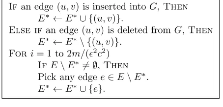
Suppose that an edge (u, v) is inserted into the graph
G = (V, E). To handle this edge insertion, we first update the listsneighbors(u) andneighbors(v), and then process the edge as follows.
• Case 1: Either Type(u) = tight or Type(v) = tight.
We do nothing and conclude the procedure.
• Case 2: Both Type(u) = slack and Type(v) = slack.
– Case 2a: Either #Friends(u) ≥ c or #Friends(v)≥c.
If#Friends(u)≥c, then we setType(u)←
tight. Next, if #Friends(v)≥c, then we set Type(v)←tight.
– Case 2b: Both #Friends(u) < c and #Friends(v)< c.
We add the edge (u, v) to the kernelκ(G) and make u, v friends of each other. Specifically, we add the node u to the list Friends(v) and v to the list Friends(u), update the pointersPointer[u, v] andPointer[v, u] ac-cordingly, and increment each of the counters
#Friends(u),#Friends(v) by one unit.
Lemma 4.1. Suppose that an edge is inserted into the
graph Gand we run the procedure described above.
1. This causes at most one edge insertion intoκ(G) and at most one edge deletion from κ(G).
2. The procedure runs inO(1)time in the worst case.
4.2.2 Handling an edge deletion inGduring the phase.
Suppose that an edge (u, v) is deleted from the graph
G = (V, E). To handle this edge deletion, we first update the listsneighbors(u) andneighbors(v), and then proceed as follows.
We check if the edge (u, v) was part of the kernel
κ(G), and, if yes, then we delete (u, v) from κ(G). Specifically, we delete u from Friends(v), v from Friends(u) (using Pointer[u, v] and Pointer[v, u]), and decrement each of the counters #Friends(u),
#Friends(v) by one unit.
We then process the nodes u and v one after another. Below, we describe only the procedure that runs on the node u. The procedure for the node v is exactly the same.
• Case 1: Type(u) = tight. Here, we check if the number of friends of uhas dropped below the prescribed limit due to the edge deletion, and, accordingly, we consider two possible sub-cases.
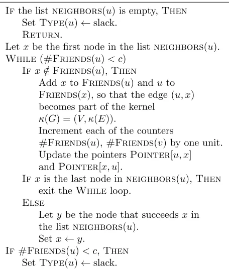
– Case 1a: #Friends(u)<(1−)c. Here, we call the subroutine REFILL(u) as described in Figure 2.
– Case 1b: #Friends(u) ≥ (1 −)c. In this case, we do nothing and conclude the procedure.
• Case 2: Type(u) = slack. In this case, we do nothing and conclude the procedure.
Lemma 4.2. Suppose that an edge is deleted from the
graph Gand we run the procedure described above.
1. This causes at mostO(c)edge insertions intoκ(G) and at most one edge deletion from κ(G).
2. The procedure runs inO(c)time in the worst case.
4.2.3 Proof of Theorem 4.2.
The first part of the theorem immediately follows from Lemmas 4.1, 4.2. We now focus on the second part. Note that at most one edge is deleted from κ(G) after an update (edge insertion or deletion) in G. Since the phase lasts for2c2/2 updates inG, at most2c2/2 edge deletions occur inκ(G) during the phase. To complete the proof, we will show that the corresponding number of edge insertions inκ(G) is alsoO(2c2).
For an edge insertion in G, at most one edge is inserted into κ(G). For an edge deletion in G, there can be O(c) edge insertions in κ(G), but only if the subroutine REFILL(.) is called. Lemma 4.3 shows that at mostccalls are made to the subroutine REFILL(.) during the phase. This implies that at most O(2c2)
edge insertions occur in κ(G) during the phase, which proves the second part of the theorem.
Lemma 4.3. The subroutine REFILL(.) is called at
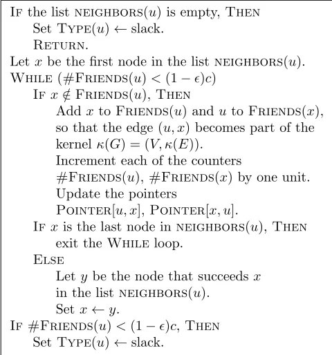
Ifthe listneighbors(u) is empty,Then SetType(u)←slack.
Return.
Letxbe the first node in the listneighbors(u). While(#Friends(u)< c)
Ifx /∈Friends(u),Then
AddxtoFriends(u) anduto
Friends(x), so that the edge (u, x) becomes part of the kernel
κ(G) = (V, κ(E)).
Increment each of the counters
#Friends(u),#Friends(v) by one unit.
Update the pointersPointer[u, x] andPointer[x, u].
Ifxis the last node inneighbors(u),Then exit theWhileloop.
Else
Lety be the node that succeedsxin the listneighbors(u).
Setx←y.
[image:16.612.68.296.75.345.2]If #Friends(u)< c,Then SetType(u)←slack.
Figure 2: REFILL(u).
Proof. When the phase begins, every tight node has exactly c friends (see Theorem 3.5), and during the phase, the status of a node u is changed from slack to tight only when |κ(Nu)| becomes (weakly) greater
thanc. On the other hand, the subroutineREFILL(u) is called only when u is tight and |κ(Nu)| falls below
(1−)c. Thus, each call to REFILL(.) corresponds to a scenario where a tight node has lost at least c
friends. Each edge deletion in Gleads to at most two such losses (one for each of the endpoints), whereas an edge insertion in G leads to no such event. Since the phase lasts for2c2/2 edge insertions/deletions inG, a
counting argument shows that it can lead to at most (2c2/2)·2/(c) =ccalls to
REFILL(.).
It remains to prove the final part of the theorem, which states that the algorithm maintains an (, c )-kernel. Specifically, we will show that throughout the duration of the phase, the subgraph κ(G) maintained by the algorithm satisfies Invariants 4–6.
Lemma 4.4. Suppose thatκ(G)satisfies Invariants 5, 6
before an edge update in G. Then these invariants continue to hold even after we modify κ(G) as per the procedure in Section 4.2.1 (resp. Section 4.2.2).
Proof. Follows from the descriptions of the procedures in Sections 4.2.1 and 4.2.2.
Recall that in the beginning of the phase, the graph
κ(G) is a (0, c)-kernel ofG. Since every (0, c)-kernel is also an (, c)-kernel, we repeatedly invoke Lemma 4.4 after each update inG, and conclude thatκ(G) satisfies Invariants 5, 6 throughout the duration of the phase. For the rest of this section, we focus on proving the remaining Invariant 4.
Fix any node v ∈ V. When the phase begins, the subgraph κ(G) is a (0, c)-kernel of G, so that we have
|κ(Nv)| ≤c. During the phase, the nodevcan get new
friends under two possible situations.
1. An edge incident to v has just been inserted into (resp. deleted from) the graphG, and the procedure in Section 5.2.3 (resp. the subroutine REFILL(v)) is going to be called.
2. The subroutine REFILL(u) is going to be called for some u∈ Nv.
If we are in situation (1) and the nodevalready has at least c friends, then the procedure under considera-tion will not end up adding any more node to κ(Nv).
Thus, it suffices to show that the node v can get at most c new friends during the phase under situation (2). Note that each call to REFILL(u), u 6= v, cre-ates at most one new friend for v. Accordingly, if we show that the subroutine REFILL(.) is called at most
ctimes during the entire phase, then this will suffice to conclude the proof of Theorem 4.2. But this has already been done in Lemma 4.3.
5 (4 + )-approximate matching in O(m1/3/2)
worst-case update time
Fix any ∈ (0,1/6). We present an algorithm for maintaining a (4 + )-approximate matching M in a dynamic graph G= (V, E) withO(m1/3/2) worst-case update time.
5.1 Overview of our approach.
As in Section 4.1, we partition the sequence of updates (edge insertions/deletions) inGintophases. Each phase lasts for 2c2/2 consecutive updates in G. Let G
i,t
denote the state ofGjust after thetthupdate in phasei.
The initial state of the graph, before it starts changing, is given by G1,0. Thus, we reach the graph Gi,t from
Gi,0 after a sequence of (i−1)·(2c2/2) +tupdates in
G.
For the rest of this section, we focus on describing our algorithm for any given phase i ≥ 1. We define
m ← |Ei,0| to be the number of edges in the input