warwick.ac.uk/lib-publications
Original citation:
Pastor-Fernandez, Carlos, Bruen, Thomas, Widanage, Widanalage Dhammika, Gama-Valdez,
M. A. and Marco, James. (2016) A study of cell-to-cell interactions and degradation in
parallel strings : implications for the battery management system. Journal of Power Sources,
329 . pp. 574-585.
Permanent WRAP URL:
http://wrap.warwick.ac.uk/81616
Copyright and reuse:
The Warwick Research Archive Portal (WRAP) makes this work of researchers of the
University of Warwick available open access under the following conditions.
This article is made available under the Creative Commons Attribution 4.0 International
license (CC BY 4.0) and may be reused according to the conditions of the license. For more
details see:
http://creativecommons.org/licenses/by/4.0/
A note on versions:
The version presented in WRAP is the published version, or, version of record, and may be
cited as it appears here.
A Study of Cell-to-Cell Interactions and Degradation in Parallel Strings:
Implications for the Battery Management System
C. Pastor-Fern
andez
a,*, T. Bruen
a, W.D. Widanage
a, M.A. Gama-Valdez
b, J. Marco
aaWMG, University of Warwick, Coventry, CV4 7AL, UK bJaguar Land Rover, Banbury Road, Warwick, CV35 0XJ, UK
h i g h l i g h t s
Experimental evaluation of SoH within parallel connected cells aged differently.
Current, SoC and cell temperature drive SoH cell-to-cell convergence.
An initial 45% difference in cell-to-cell SoH (resistance) converges to 30%.
An initial 40% difference in cell-to-cell SoH (capacity) converges to 10%.
A linear correlation between capacity fade and resistance increase is observed.
a r t i c l e i n f o
Article history: Received 6 June 2016 Received in revised form 23 July 2016
Accepted 31 July 2016
Keywords:
Lithium ion technology Battery pack
Battery management system State of health estimation
a b s t r a c t
Vehicle battery systems are usually designed with a high number of cells connected in parallel to meet the stringent requirements of power and energy. The self-balancing characteristic of parallel cells allows a battery management system (BMS) to approximate the cells as one equivalent cell with a single state of health (SoH) value, estimated either as capacity fade (SoHE) or resistance increase (SoHP). A single SoH value is however not applicable if the initial SoH of each cell is different, which can occur when cell properties change due to inconsistent manufacturing processes or in-homogeneous operating environ-ments. As such this work quantifies the convergence of SoHEand SoHPdue to initial differences in cell SoH and examines the convergence factors. Four 3 Ah 18650 cells connected in parallel at 25C are aged
by charging and discharging for 500 cycles. For an initial SoHEdifference of 40% and SoHPdifference of 45%, SoHEconverge to 10% and SoHPto 30% by the end of the experiment. From this, a strong linear correlation betweenDSoHEandDSoHPis also observed. The results therefore imply that a BMS should consider a calibration strategy to accurately estimate the SoH of parallel cells until convergence is reached.
©2016 Published by Elsevier B.V.
1. Introduction
In recent years lithium-ion (Li-ion) cells in a battery pack have become the favourable choice for electric power transportation systems. In order to increase the pack capacity and meet re-quirements for power and energy, cells in a battery module are often electrically connected in parallel[1]. For instance, each unit of the BMW E-Mini 35 kWh battery pack is composed of 53 cells connected in parallel and 2 in series. Two units constitutes a module and the whole battery is composed of 48 modules con-nected in series[2]. Another example is the Tesla Model S 85 kWh
battery pack. This battery pack includes 16 modules of 6S74P configuration (6 cells connected in series and 74 cells connected in parallel) summing to 7104 cells within the complete battery as-sembly[3].
Battery health diagnosis is essential to develop a control strat-egy in order to ensure safe and lifetime efficient operation of electric and hybrid vehicles. State of Health (SoH) is the parameter used by the Battery Management System (BMS) to monitor battery ageing. SoH is often calculated based on two metrics: capacity fade and power fade[4]. These metrics are directly related to vehicle level attributes that limit driving range and vehicle power, respectively. For the case where cells are connected in parallel, the BMS typically does not monitor the SoH of each individual cell because the BMS does not have access to individual cell currents *Corresponding author.
E-mail address:[email protected](C. Pastor-Fernandez).
Contents lists available atScienceDirect
Journal of Power Sources
j o u r n a l h o me p a g e :w w w . e l s e v i e r . c o m / lo c a t e / j p o w s o u r
http://dx.doi.org/10.1016/j.jpowsour.2016.07.121
and temperatures. Thus, the BMS cannot determine the capacity fade and power fade at cell level. For this case the BMS approxi-mates the SoH as that of an equivalent single value for the whole battery stack. This approximation is based on the assumption that the SoH of cells connected in parallel are the same since they have identical terminal voltages. This assumption is however no longer valid when cell properties change due to manufacturing tolerances and usage conditions. For instance, the presence of temperature gradients or the existence of different resistance paths that will underpin an uneven current distribution within the system repre-sent typical scenarios where cell-to-cell SoH may be different. Such an imbalanced scenario has been previously examined in Refs.[5e8]. Another potential application of this study is second life grid storage modules connected in parallel as suggested in Refs.[9,10].
In a recent study, Gogoana et al. [5] cycled two cylindrical lithium-iron phosphate (LFP) cells connected in parallel to evaluate the degradation of each cell over time. They identified that an initial 20% discrepancy in internal resistance between cells in a parallel string results in a 40% reduction of the total cycle life. They attributed this result to the uneven high currents experienced by each cell.
Gong et al.[6]cycled four groups of Li-ion cells. Each group of cells was composed of two cells with different degradation levels. They showed that when two cells with a 20% impedance difference were connected in parallel, the peak current experienced was 40% higher than if the cells had the same impedance.
Zhang et al.[7]cycled two 26650 LFP cells connected in parallel, with each cell at a different temperature (5C and 25C). Based on a simplified thermal-electrochemical model, it was shown that temperature differences between the cells makes self-balancing difficult, which consequently accelerates battery degradation.
Shi et al. [8] cycled two groups of LFP batteries (each one composed of two cells) for cycle life and basic performance anal-ysis. Thefirst group was tested at 25C, whereas the second group was tested at 25C and 50C to evaluate the effect of high tem-perature. They concluded that imbalanced currents can directly affect the capacity fade rate of cells connected in parallel.
These studies highlight that cells connected in parallel will age differently when the SoH of each individual cell is not the same. These results raise the question as to whether the BMS will esti-mate the SoH correctly under this situation. The contribution of this work is tofind an answer for this question quantifying the cell-to-cell SoH for a scenario when each initial cell-to-cell SoH is different. To understand the reasons behind the cell-to-cell SoH variation, SoC, current and temperature distribution in the short-term, and charge-throughput and thermal energy in the long-term are examined. A simple SoH diagnosis and prognosis approach is also presented, where capacity and resistance, and the change in SoHE (based on a measure of the cell capacity) and the change in SoHP (based on a measure of the cell resistance) are approximated by a linear relationship. The overall output of this work is expected to improve the accuracy of SoH diagnosis and prognosis functions within the BMS when cells are connected in parallel.
The structure of this work is divided as follows: Section2 ex-plains the most common definitions used in the literature for SoH capacity fade (SoHE) and power fade (SoHP). Section3summarises
the experiment where four commercially available 3 Ah 18650 lithium-ion cells connected in parallel were aged by 500 cycles. The results are given in Section4, where the factors which drive the SoH convergence are evaluated. Based on the results for capacity and resistance fade, Section 5 proposes a simple approach for SoH diagnosis and prognosis based on a linear correlation between capacity and resistance, and between the change in SoHE(
D
SoHE) and the change in SoHP(D
SoHP). Finally, the limitations of thisstudy and further work are stated in Section6and conclusions are presented in Section7.
2. SoH definition
SoH diagnosis and prognosis is essential to ensure effective control and management of Li-ion Batteries (LIBs). The SoH will evolve differently depending on the battery state: cycling or storage [11]. The SoH depends also on different parameters which can be controlled by the BMS. For automotive applications these param-eters are typically battery temperature, Depth of Discharge (DoD), discharging and charging current rates for cycling, and the SoC employed for storage conditions [4]. Since the SoH depends on different parameters it is difficult to estimate the contribution of each parameter. The SoH has an upper and a lower limit: Begin of Life (BoL) and End of Life (EoL). BoL (SoH¼100%) represents the state when the battery is new, and EoL (SoH¼0%) is defined as the condition when the battery cannot meet the performance specifi -cation for the particular appli-cation for which it was designed[13]. In essence, EoL corresponds to the battery End of Warranty (EoW) period, adopted in some automotive standards[14,15]. In relation to capacity and resistance, the EoL values are commonly defined as [4,11e13]:
CEoL¼0:8$CBoL (1)
REoL¼2$RBoL (2)
According to[4]and[11e13],SoHEandSoHPare often calculated
as a percentage with respect to the difference between BoL and EoL in either capacity (Equation(3)) or resistance (Equation(4)).
SoHE¼
CnowCEoL
CBoLCEoL$
100¼Cnow0:8$CBoL
CBoL0:8$CBoL$
100
¼Cnow0:8$CBoL
0:2$CBoL $
100 (3)
SoHP¼RRnowREoL BoLREoL$
100¼Rnow2$RBoL
RBoL2$RBoL$
100
¼
2Rnow
RBoL
$100 (4)
The decision as to which measure of battery health to use,SoHE,
SoHPor both, depends on the application. In the case of the
auto-motive industrySoHEis commonly employed in high-energy
ap-plications such as BEVs (specific energy>150 Wh/kg)[16],SoHPis
used for high-power applications such as Hybrid Electric Vehicles (HEVs) (specific power>1500 W/kg)[16]and both metrics can be combined for Plug-in-HEV (PHEV) applications.
3. Experimental procedure
This study extends the experiment performed in[1], where four 3 Ah 18650 Li-ion cells were aged by 0, 50, 100 and 150 cycles individually to ensure an initialSoHEdifference of 40% andSoHP
difference of 45% between the least and the most aged cells. These values correspond to a difference of capacity and impedance of circa 8% and 30% respectively. Research published highlights that differences in cell properties from initial manufacture and inte-gration may be circa 25% for impedance[5]and 9% for capacity[17], which is in agreement with the initial differences considered in this study. The four cells are then connected in parallel and cycled for a total of 500 cycles, where 500 cycles represents the EoL state ac-cording to the manufacturer's specifications. Thus, all the cells were loaded at least for 500 cycles. The experimental procedure is
divided into two phases: cycle ageing and cell characterisation. Table 1 shows the test that was performed. The following sub-sections summarise each of these tests. For a more detailed explanation, refer to[1].
3.1. Cycle ageing
As illustrated inFig. 1(a) cycle ageing involved repeated cycles at constant ambient temperature of 25C±1C of the following: a 1 C discharge until the lower voltage limit was reached followed by Constant Current-Constant Voltage (CC-CV) charging protocol. The CC phase involved charging the cell at C/2 until the end of charge voltage (4.2 V) was reached. The CV phase then consisted of charging the cell until the current fell to C/20 (150 mA). This profile was selected to significantly age the cells whilst not exceeding the
manufacturer's operating cell specification. This was achieved by cycling the cells with a full DoD (e.g. 0e100%) without using large currents[1]. A large DoD is deemed to emulate the operation of a typical BEV in which, as discussed within[1], the BMS will control a large variation in SoC to further maximise the range of the vehicle. During cycle ageing, each cell was connected in series with a 10 m
U
shunt resistor over which the voltage was measured. The current was then calculated based on a current-voltage relationship obtained through a least-squares solution in Ref.[1]. In addition, the temperature was also measured midway along its length of each cell using type T thermocouples.3.2. Cell characterisation
Cell characterisation includes three tests: capacity test,
pseudo-Table 1
Experimental test matrix.
[image:4.595.35.555.638.733.2]Cell Test Test starta
[#cycles]
Testfinish [#cycles]
Testing procedure T
[C] D
DoD [%]
tsamp
[s]
1 Cycling 0 500 CC-CV chg and 1C dchg 25 100 1
Charact Every 50 cycles 1C dchg, EIS test and pseudo-OCV 25 100 1
2 Cycling 50 500 CC-CV chg and 1C dchg 25 100 1
Charact Every 50 cycles 1C dchg, EIS test and pseudo-OCV 25 100 1
3 Cycling 100 500 CC-CV chg and 1C dchg 25 100 1
Charact Every 50 cycles 1C dchg, EIS test and pseudo-OCV 25 100 1
4 Cycling 150 500 CC-CV chg and 1C dchg 25 100 1
Charact Every 50 cycles 1C dchg, EIS test and pseudo-OCV 25 100 1 aInitial testing was performed in Ref.[1].
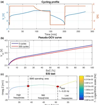
Fig. 1.(a) Charge-discharge cycling profile employed to age the cells, (b) Pseudo-OCV-SoC curve of cell 1 for 0 and 500 cycles for a discharge event, (c) EIS test with respect to the frequency showing BMS operating area andRBMS.
OCV test and EIS test. In order to track the aged state of each cell over time, each of these tests was performed every 50 cycles. In total, each cell was characterised 11 times.
The capacity test determines the quantity of electric charge that a battery can deliver under specified discharge conditions. Firstly each cell was charged to 100% SoC according to CC-CV protocol. Then, the cell was discharged at 1 C to the lower voltage limit. The cell's capacity is defined as the charge dissi-pated over this discharge event.
The pseudo-OCV test is performed by discharging from the upper cell voltage threshold (4.2 V) to the lower cell voltage threshold (2.5 V) at C/10. The corresponding pseudo-OCV curve is related to the SoC and is shown for cell 1 for 0 and 500 cycles inFig. 1(b).
The EIS test was performed in galvanostatic mode with a peak current amplitude of 150 mA (C/20) using a Solartron modulab system (model 2100A). The tests were performed between 2 mHz and 100 kHz at SoC¼20%, SoC¼50% and SoC¼90%. SoC was adjusted based on the pseudo-OCV curve (refer toFig. 1(b)). According to[18], a period of 4 h was allowed prior to per-forming each EIS test. This measure avoids changes in the in-ternal impedance when the cells are halted after being excited. Operation at high frequencies (2.5 kHz) would increase sub-stantially the cost of the BMS hardware because the required sampling rate will be higher. This explains why a BMS will typically only operates at mid and low frequencies (<100 Hz). As such, the resistance considered for this work is the one that the BMS is capable of measuring. This resistance is here named as a
BMS resistance (RBMS) and, it is represented by the
mid-frequency turning point of the EIS plot as illustrated in Fig. 1(c). This approach is consistent with other studies reported within the literature[1],[19].
4. Results and discussions
4.1. CapacityeSoHEand resistanceeSoHP
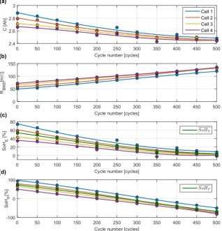
Fig. 2(a) and (b) illustrate the degradation of each cell over time based on the measurement of the capacity at 1 C and theRBMSat an
SoC of 50%.
Fig. 2(a) and (b) indicate that capacity and RBMS tends to
converge for cells 2, 3 and 4 over cycle number. Since cell 1 rep-resents the least aged cell, it requires more time to converge at the same level than the rest of the cells.Fig. 2(c) and (d) show that the resultingSoHEandSoHPtrend is similar to the capacity andRBMS
trend. It can be seen that the SoHP decreases faster than SoHE
reaching the EoL value earlier (between 200 and 350 cycles) than the value specified by the manufacturer (500 cycles). This result indicates the lifetime power capability of the cells is shorter than the energy capability.SoHPdecreases faster thanSoHEbecause the
conditions at which the cells were cycled (1C-rate discharge and
D
DoD¼100%) leads to significant power losses. Such a cell would not meet a commercial viable battery specification where both metrics,SoHEandSoHP, need to be positive until the EoW period isreached.
[image:5.595.145.464.394.726.2]Fig. 2(c) and (d) also illustrate the mean value of the SoH. This value represents the equivalent SoH that the BMS would track. A
new metric called State of Imbalance (SoI) is defined to quantify the maximum cell-to-cell SoH difference at each characterisation testk. The SoI is calculated for the case of SoHE and SoHP as shown
Equation(5)and Equation(6).
SoIkE¼maxSoHEkminSoHEk (5)
SoIk P¼max
SoHk
P
minSoHk
P
(6)
k¼1:::11
Fig. 3(a) illustrates thatSoIPdecreases less than theSoIE. For an
initialSoIEof 40% andSoIPof 45%,SoIEdecreases to 10% andSoIPto
30% by the end of the test. In order to study which cell contributes more to theSoHconvergenceFig. 3(b) and (c) show the difference of each cell SoHEandSoHPwith respect to the mean value
illus-trated inFig. 2(c) and (d), respectively.ContEandContPof each celli
at each characterisation testkis computed using Equation(7)and Equation(8).
ContkE i¼SoHE ik SoHk
E i (7)
ContkP i¼SoHP ik SoHk
P i (8)
k¼1:::11; i¼1:::4
Fig. 3(b) and (c) show cell 1, the least aged cell, contributes more
to the convergence whilst cell 4, the most aged cell, contributes the least. TheContEandContPdecreases with cycle number, outlining
the SoH of each cell tends to converge.
4.2. Driving factors for SoH convergence
4.2.1. Current and charge-throughput distribution
Previous work[1]showed that cells connected in parallel under imbalanced scenarios can undergo significantly different currents, contributing to the cells degrading differently. To understand the variation of the individual cell currents when the cells are con-nected in parallel a simplified cell model was here considered. This model comprises an OCV voltage sourceVoc connected in series
with an internal cell resistanceRint. Previous literature[1,12,18,19]
use this model with an added RC parallel branch to capture diffu-sion effects. The RC parallel combination is herein neglected to help explain the cell-to-cell SoH variation more easily.
Based on this model, the individual cell current is derived as in Equation(9).
Vt¼VocþVR¼VocþRint$Icell/Icell¼
VtVoc
Rint
(9)
The wide SoC range and difference in cell SoH give a scenario with significant differences in Voc and Rint which, according to
Equation(9), will cause differences in cell currents.
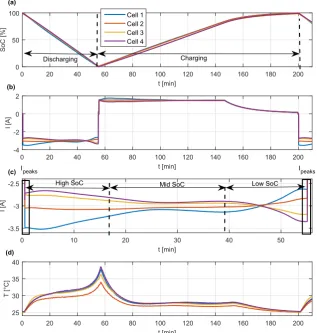
Fig. 4(a) and (b), andFig. 5(a) and (b) relate the individual SoC and the individual cell currents of each cell I1, I2, I3and I4for the 35thand the 435thdischarge-charge cycle, respectively. These cy-cles were arbitrarily selected near to the beginning and the end of Cycle number [cycles]
0 50 100 150 200 250 300 350 400 450 500
SoI [%]
0 20 40 60
SoIE SoIP
Cycle number [cycles]
0 50 100 150 200 250 300 350 400 450 500
Cont
E
[%]
-30 -20 -10 0 10 20
30 Cell 1
Cell 2 Cell 3 Cell 4
Cycle number [cycles]
0 50 100 150 200 250 300 350 400 450 500
Cont
P
[%]
-30 -20 -10 0 10 20 30 (b)
[image:6.595.135.452.67.396.2](c) (a)
Fig. 3.(a)SoIEandSoIPover cycle number, (b) CellContEover cycle number and (c) CellContPover cycle number.
the test.
The individual current of each cell diverges more for the dis-charging event than for the dis-charging event because the magnitude of the C-rate is larger for discharging (1 C) than for charging (þ0.5 C). The SoC of the less aged cells (cells 1 and 2) decreases during discharging or increases during charging faster than for the more aged cells because the currentflow in the less aged cells is higher in magnitude than in the more aged cells (cells 3 and 4). Thus, when the less aged cell has completely discharged (or charged), the more aged cells have not discharged (or charged) completely yet, which consequently may drive higher currents in these cells.
According to [1], this uneven current distribution during charging and discharging causes peaks in the current which could lead to premature ageing of the cells.Fig. 4(c) andFig. 5(c) illustrate the current distribution of each cell during discharge for the 35th and the 435th discharge-charge cycle, respectively. The peaks in the current are reached at low and high SoC, as a result of the deepest discharge effects of the pseudo-OCV curve (refer toFig. 1(b)). The less aged cells take more current at high SoC as their impedance is lower than the impedance of the more aged cells. However, the more aged cells take more current at low SoC as they have been discharged slower than the less aged cells and thus their imped-ance is lower than the impedimped-ance of the less aged cells. According toFig. 1(b), theVocalso decreases more at low SoC that additionally
limits the current that is able toflow (refer to Equation(9)). This trade-off between SoC, impedance andVocexplain the cell-to-cell
current cross-over depicted inFig. 4(c) and Fig. 5(c). This result
has been previously reported in Refs.[1],[5].
Another observation fromFig. 4(c) andFig. 5(c) is the peak-to-peak current difference between the 35thand the 435thcycle. The peak-to-peak current difference between the least and the most aged cell is larger at high SoC or low SoC for the 35thcycle (0.75 A) than for the 435thcycle (0.5 A). This convergence in the peak-to-peak current is explained by the convergence of the individual cell capacity and resistance as illustrated inFig. 2(a) and (b).
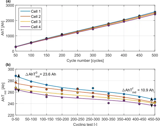
The charge-throughput is evaluated to analyse the effect of the current distribution in the long-term. The charge-throughput is the amount of accumulated current (absolute value) that is stored (charging) and released (discharging) in the battery over time. Using Equation (10) the charge-throughput is computed as the integral of the current over the difference between thefinaltk
f and
the initial tk
0 time. In this case, as the cycling test is“paused”to characterise the cells, the charge-throughput (AhT) over the total cycling tests is derived as the monotonic accumulation of the charge-throughput of each individual cycling test k, one after another.
AhTik¼Xk
k¼1
Ztk f
tk
0
IðtÞk
idt (10)
k¼1:::11; i¼1:::4
Fig. 6(a) illustrates the charge-throughput of each cell i over t [min]
0 20 40 60 80 100 120 140 160 180 200
SoC [%]
0 50
100 Cell 1
Cell 2 Cell 3 Cell 4
t [min]
0 20 40 60 80 100 120 140 160 180 200
I [A]
-4 -2 0 2
t [min]
0 10 20 30 40 50
I [A]
-3.5 -3 -2.5
t [min]
0 20 40 60 80 100 120 140 160 180 200
T [°C]
25 30 35 40
Discharging Charging
Ipeaks Ipeaks
(a)
(b)
(c)
(d)
[image:7.595.145.463.68.402.2]High SoC Mid SoC Low SoC
Fig. 4.(a) Individual SoC of each cell for the 35thcycle, (b) current distribution of each cell for the 35thcycle, (c) detailed view of this current distribution for the discharge event for the 35thcycle, (d) temperature distribution of each cell for the 35thcycle.
t [min]
0 20 40 60 80 100 120 140 160 180 200
SoC [%]
0 50
100 Cell 1Cell 2 Cell 3 Cell 4
t [min]
0 20 40 60 80 100 120 140 160 180 200 Icell
[A]
-2 0 2
t [min]
0 5 10 15 20 25 30 35 40 45 50
Icell
[A]
-3.2 -3 -2.8
t [min]
0 20 40 60 80 100 120 140 160 180 200 Tcell
[°C]
25 30 35 40 (c)
(d) (b) (a)
Ipeaks
Low SoC Mid SoC
High SoC Ipeaks
[image:8.595.134.454.65.392.2]Discharging Charging
Fig. 5. (a) Individual SoC of each cell for the 435thcycle, (b) current distribution of each cell for the 435thcycle, (c) detailed view of this current distribution for the discharge event for the 435thcycle, (d) temperature distribution of each cell for the 435thcycle.
Cycle number [cycles]
50 100 150 200 250 300 350 400 450 500
AhT [Ah]
0 1000 2000 3000
Cell 1 Cell 2 Cell 3 Cell 4
Cycling test [-]
0-50 50-100 100-150 150-200 200-250 250-300 300-350 350-400 400-450 450-500
AhT
ind
[Ah]
220 240 260 280 300
AhTind0 = 23.6 Ah (a)
(b)
AhTindf = 10.9 Ah
Fig. 6.(a) Accumulative charge-throughput taken by each cell over cycle number, (b) Charge-throughput taken by each cell over each cycling test. C. Pastor-Fernandez et al. / Journal of Power Sources 329 (2016) 574e585
[image:8.595.133.448.466.714.2]cycle number and show that the charge-throughput of the less aged cells is larger than for the more aged cells over time, outlining the current in the less aged cells is in overall larger than in the more aged cells.
To see clearly that the charge-throughput also converges the individual charge-throughput after each cycling test is computed using Equation(11). Equation(11)is the same than Equation(10) without accumulating the charge-throughput over cycle number.
AhTi indk ¼
Ztk f
tk
0
IðtÞk
idt (11)
k¼1:::11; i¼1:::4
Fig. 6(b) illustrates that the individual charge-throughput after each cycling test converges. This result together with the conver-gence of the current (short-term) support the converconver-gence of the SoH.
4.2.2. Temperature and thermal-energy distribution
Since cell temperature primarily depends on cell impedance and current, a number of studies correlate these parameters with SoH [1,7,8].Fig. 4(d) andFig. 5(d) show the temperature distribution in each cell for the 35th and the 435th charge-discharge cycle, respectively.
Fig. 4(d) andFig. 5(d) illustrate that the cell temperature is larger for all the cells at the 435th(43C) than the 35thcycle (38C). The increase in temperature over cycle number is due to the increase of RBMS as depicted inFig. 2. This increase of temperature is more
significant for low and high SoC with respect to mid SoC due to the divergence of the individual cell currents (refer to Section4.2.1) and larger magnitude of RBMS[19].
In comparison with the current depicted in Fig. 4(d) and Fig. 5(d), the variation of the temperature does not follow the initial order of ageing of each cell.Fig. 4(d) depicts that the temperature of cell 1, cell 3 and cell 4 is larger than the temperature of cell 2. This result is explained based on the relative values of the impedance of each cell with respect to the current. The difference in current of cell 1, cell 3 and cell 4 vary significantly (
D
I1¼0.9 A,D
I3¼0.42 A andD
I4 ¼ 0.65 A) from the beginning to the end of the discharge, whereas the difference in current of cell 2 changes less (D
I2¼0.2 A). In addition, the change of the impedance with respect to the SoC influences also in the variation of cell temperature. For instance, since cell 1 is the least aged cell it has the lowest resistance value (refer toFig. 2(b)). However, the impedance of cell 1 will rise at low SoCs due to the significant drop ofVoc(refer toFig. 1(b)) causing anincrease in temperature. The temperature of cell 2 is consistently the lowest temperature because it has a relatively low impedance without undergoing large current differences. This result is sup-ported in Ref.[1]where cell temperature did not vary with respect to the order of ageing.
For the case of the 435thcycle, the temperature is approximately the same for all the cells since the current from the beginning to the end of the discharge change very little (
D
I1¼0.4 A,D
I2 ¼0.04 A,D
I3¼0.15 A andD
I4¼0.3 A) and the resistance of each cell tend to converge (refer to cell resistance values inFig. 2(b)). Comparing bothFig. 4(d) andFig. 5(d) it is possible to conclude that temper-ature tend to converge over time.It can also be seen that the average peak temperature at 435th cycle (41.5C) is larger than the average peak temperature at 35th cycle (36C) due to the increase ofRBMSwith cycle number (refer to
Fig. 2(b)). To evaluate the temperature convergence in the long-term Equation (12) approximates the total thermal energy
released in each cellialong the total number of cycling tests.
Eth ik ¼Xk
k¼1
Ztk f
tk
0
IðtÞk
i
2
$Rk
BMS idt (12)
k¼1:::11; i¼1:::4
WhereIðtÞk
i denotes the currentflow, andt0kandtkf the initial and
thefinal time. Equation(13)givesRk
BMSas the mean value of the
instantaneous RBMS for each characterisation test k and cell i
considering each measured SoC.
Rk BMS i¼
Rk
BMS i20%þRkBMS i50%þRkBMS i90%
3 (13)
k¼1:::11; i¼1:::4
The RMS value of the current is employed to simplify Equation (12) and it was calculated using Equation(14)over the charge-discharge cycle periodT.
Ik RMS i¼
ffiffiffiffiffiffiffiffiffiffiffiffiffiffiffiffiffiffiffiffiffiffiffiffiffiffiffiffiffiffiffiffiffiffiffiffiffiffiffiffi
1
Tk
Ztk f
tk fTk
IðtÞk
i 2 dt v u u u u u t (14)
k¼1:::11; i¼1:::4
The thermal energy based on the RMS value of the current is computed using Equation(15).
Eth ik ¼Xk
k¼1
IRMS ik 2$Rk BMS i$
tfkt0k (15)
k¼1:::11; i¼1:::4
Similarly as with the charge-throughput, the thermal energy was computed as the monotonic accumulation of the thermal en-ergy of each individual cycling testk, one after another.Fig. 7(a) demonstrates the thermal energy released by the more aged cells is larger than the thermal energy released by the less aged cells. The least aged cell (cell 1) typically undergoes the highest current, having the lowest impedance. Likewise, the most aged cell (cell 4) typically undergoes the lowest current, having the highest impedance. Thus, this result indicates theRBMScontributes more to
the thermal energy than the I2
RMS. To compare the contribution
betweenRBMSandIRMS2 the ratio between theRBMSfor cell 4 and cell
1 for each characterisation testk, and the ratio between theI2
RMSfor
cell 1 and cell 4 for each characterisation testkare derived using Equation(16)and Equation(17).
Rkr BMS¼RkBMS i¼4
Rk BMS i¼1
(16)
Ir RMSk ¼
Ik
RMS i¼1
2
Ik
RMS i¼4
2 (17)
k¼1:::11
Fig. 7(b) illustratesRk
r BMSis for the major part of the test larger
thanIk
r RMS suggesting that thermal energy is more sensitivity to
RBMSthan toIRMS2 .
To see clearly that the thermal energy also converges over time, the individual thermal energy released after each cycling test is computed using Equation (18). Equation (18) is the same than Equation(15)without accumulating the thermal energy over cycle number.
Ekth ind i¼IRMS ik 2$Rk BMS i$
tfkt0k (18)
k¼1:::11; i¼1:::4
Fig. 7(c) depicts the thermal energy released by each cell over each cycling test converges. Hence, the convergence of temperature (short-term) together with the convergence of the thermal energy (long-term) support the convergence of the SoH.
As an overview,Table 2gives a summary of the results evaluated in this section, highlighting the values at the beginning and at the
end of the experiment. Observed that the capacity andRBMSof the
cells before being connected in parallel differ with respect to the values reported in Ref.[1]. Since the cells were stored over half a year between the previous and this study, this difference is attributed to calendar ageing effects.
5. Simplified approach to SoH diagnosis and prognosis for cells connected in parallel
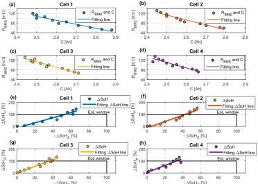
Previous studies[20,21], found that knowing the capacity allows the resistance to be approximated, and vice versa. In support of those studiesFig. 8(a), (b), (c) and (d) show a correlation between capacity andRBMS for each cell. This correlation follows a linear
[image:10.595.135.447.69.336.2]trend since it can be approximated by afirst-order polynomialfit. To measure the goodness offit of this linear relationship the R-square value is used. The R-R-square can vary between 0 and 1, where 0 indicates that the model describes none of the variability of the Fig. 7.(a) Total thermal energy taken by each cell over cycle number, (b) comparison betweenRk
[image:10.595.38.552.407.480.2]r BMSandIr RMSk over cycle number, (c) total thermal energy taken by each cell over each cycling test.
Table 2
Test results for the cells before and after being connected in parallel.
Cell Test start Testfinish
Ca,b
[Ah]
RBMSa,c
[mU]
AhTd
[kAh]
Ethe
[kJ]
SoHEf
[%]
SoHpg
[%]
Ca,b
[Ah]
RBMSa,c
[mU]
AhTd
[kAh]
Ethe
[kJ]
SoHEf
[%]
SoHpg
[%]
1 2.88 50.72 0.00 0.00 73.68 96.54 2.54 120.00 2.55 2357.80 7.89 50.87 2 2.79 59.04 0.00 0.00 58.88 86.58 2.50 132.04 2.50 2454.30 2.96 76.13 3 2.71 66.66 0.00 0.00 42.81 79.30 2.47 131.37 2.45 2443.30 1.30 68.44 4 2.66 72.15 0.00 0.00 34.64 70.94 2.48 134.85 2.40 2493.00 1.30 81.94 aNot exactly the same values as in Ref.[1]because the cells were aged due to calendar ageing between the two different tests.
bBased on 1 C capacity test. c R
BMSmeasured at 50% SoC.
d Refer to Equation(10). eRefer to Equation(12). f Refer to Equation(3). gRefer to Equation(4).
response data with respect to its mean, and 1 indicates that the model relates all the variability of the response data with respect to its mean[21]. The minimum adjusted R-square value for all the cases analysed is 0.8831 for cell 4. This result implies the linearfits relate a significant variability of the response data with respect to their mean.
To estimate the change of SoH based on the capacity fade or the increase of resistance,
D
SoHkE i and
D
SoHP ik are calculated usingEquation(19)and Equation(20).
D
SoHkE irepresents the difference
between theSoHEof each characterisation test kand each cell i
(SoHk
E i) with respect to the SoHEof thefirst characterisation test
k¼1 and each celli(SoH1
E i). Similarly,
D
SoHkP irepresents thedif-ference between theSoHPof each characterisation testkand each
celli(SoHk
P i) with respect to theSoHPof thefirst characterisation
testk¼1 and each celli(SoH1
P i).
D
SoHkE i¼SoHkE iSoHE i1 (19)D
SoHkP i¼SoHP ik SoH1P i (20)k¼1:::11; i¼1:::4
Fig. 8(e), (f), (g) and (h) show the results for
D
SoHkE iand
D
SoHkP ifor each cell. The relationship between
D
SoHkE iand
D
SoHP ik is linearfor each cell and thus it is also approximated by a first-order polynomial fit. Similarly as the previous case, the minimum adjusted R-square value for all the cases analysed is 0.8831 for cell 4. It can also be seen that
D
SoHPgoes outside of the EoL threshold asit was illustrated inFig. 2(b). Despite this, the linear relationship between
D
SoHEandD
SoHPwill be still valid. The only differencewith respect to the result presented will be the gradient of the approximated line.
The Pearson product-moment correlation coefficient (PPMCC) is employed to quantify the grade of correlation betweenCandRBMS,
and
D
SoHPandD
SoHE[21]. Equation(21)and Equation(22)definesthe PPMCC coefficients are computed as the covariance divided by the standard deviations of each parameter using Equation(21)and Equation(22).
rRBMS;C¼
covRBMS;C
s
RBMS$sC(21)
rDSoHP;DSoHE ¼covDSoHP;DSoHE
s
DSoHP$sDSoHE(22)
The PPMCC varies between1 andþ1, depending if the corre-lation is weak or strong. The absolute value of PPMCC is considered in order to interpret the strength of the correlation as follows. Employing the commandcorrcoefin MATLAB[22], the minimum rRBMS;CandrDSoHP;DSoHE is for both cases 0.9459 for cell 4. This result
highlights that C and RBMS, and
D
SoHP andD
SoHE are stronglycorrelated.
The linear correlation provides sufficient justification to calcu-late capacity or resistance based on the knowledge of the other. Secondly, this linear correlation allows the BMS to estimate in the short-term (diagnosis) and in the long-term (prognosis) the change of SoH in a simple way, which may be further investigated in the future for real-time battery applications.
6. Limitations of this study and further work
In order to reduce the duration of the experiment, only one capacity and resistance measurement of each cell at each ageing state was considered. According to the theory of Design of Exper-iments (DoE) [23], more than one sample is recommended to ensure the measurements are representative. Thus, a greater sample size is necessary to increase confidence in thefindings of this study.
[image:11.595.116.489.65.330.2]The results of this study are only valid for the described Fig. 8.Linear correlation between capacity andRBMSat 50% SoC for (a) cell 1, (b) cell 2, (c) cell 3 and (d) cell 4. Linear correlation between increase inDSoHEandDSoHPat 50% SoC for
(e) cell 1, (f) cell 2, (g) cell 3 and (h) cell 4.
experimental conditions. In cases where the testing conditions change (e.g. ambient temperature or C-rate); or, the number of cells connected in parallel is different than four; or, the condi-tions at which the cells were initially aged are different; then, the convergence may not be reached or may be reached earlier or later. For instance, if the C-rate is high (1.5 C), then the least aged cell could undergo more current than the maximum current specified by the cell's manufacturer. This could ultimately result in a cell failure. Another example is that the number of cells connected in parallel may be related to the time required for the cells to converge. Therefore, the same study at different experimental conditions would need to be investigated in the future.
Similarly, the correlation between the capacity andRBMS, and the
change inSoHE(
D
SoHE) andSoHP(D
SoHP) could also be non-linearfor other test conditions, for instance, when cycling and storage conditions are combined. Hence, the applicability of this should also be tested against other testing conditions (cycling and storage) and other cell chemistries.
7. Conclusions
This work analysed the cell-to-cell SoH variation of four 3 Ah 18650 Li-ion cells connected in parallel. The SoH is defined by the capacity fadeSoHE, and the power fadeSoHP. For an initialSoHE
difference of 40% at the beginning of the test, the cells SoHE
converge to 10% at the end of the test (500 cycles). For the case of theSoHP, for an initial difference of 45% the cells converge to within
30% at the end of the test. The initialSoHPandSoHEcorresponds to a
difference of circa 30% in impedance and 8% in capacity, values which are in agreement with potential differences in cell properties from initial manufacture and integration[5,17]. This study high-lights that the BMS would track an incorrect value of the SoH until the convergence is reached. To understand the reasons behind the SoH convergence, the distribution of the SoC, current, temperature, charge-throughput and thermal energy were studied. The distri-bution of the cell currents does not entirely depend on the initial ageing state of each cell as it is commonly assumed. The variation depends on the OCV-SoC relationship and the change of cell impedance with respect to SoC. This non-linearity in the variation of the current may cause uneven heat generation within a pack, which may require a higher specification thermal management system[1]. In comparison with the current distribution, the vari-ation of the SoC and the temperature is less dynamic. Although these parameters change differently, all of them tend to converge over time, driving the convergence of SoH. The charge-throughput and the thermal energy of each cell over 500 cycles was also studied to analyse variation of the current and the temperature in the long-term. Similarly as for the current and the temperature, the charge-throughput and the thermal energy tend to converge over time.
This work also shows that the magnitude of the SoH decreases much faster for the case of the SoHP with respect to the SoHE
because the testing conditions employed to cycle the cells (1 C discharge and
D
DoD¼100%) leads to significant power fade.In addition, this work suggested a simple approach for SoH diagnosis and prognosis within the BMS. This approach was based on two linear correlations: one between the capacity andRBMS, and
the other between the change inSoHE(
D
SoHE) andSoHP(D
SoHP)with a minimum adjusted R-square value of 0.8831 for both cases. This result is relevant for two main reasons. Firstly, it is only necessary to measure one parameter to estimate the other. Sec-ondly, it could be further used to estimate the EoL of the battery. This would also require the analysis of the correlation under other conditions (e.g. temperature, C-rate, SoC and
D
DoD) in order tocover the whole cycling spectra that a commercial battery pack may be subject to.
Acknowledgements
The research presented within this paper is supported by the Engineering and Physical Science Research Council (EPSRC - EP/ I01585X/1) through the Engineering Doctoral Centre in High Value, Low Environmental Impact Manufacturing. The research was un-dertaken in the WMG Centre High Value Manufacturing Catapult (funded by Innovate UK) in collaboration with Jaguar Land Rover. Details of additional underlying data in support of this article and how interested researchers may be able to access it can be found here:http://wrap.warwick.ac.uk/81110.
The authors would like to thank Dr. Gael H. Chouchelamane, Dr. Mark Tucker and Dr. Kotub Uddin for the support on the experi-mental measurements and analysis of the results.
Nomenclature
Abbreviation
BEV Battery Electric Vehicle BMS Battery Management System BoL Begin of Life
CC-CV Constant Current Constant Voltage
chg Charge
Charac Characterisation dchg Discharge
DoD Depth of Discharge DoE Design of Experiment
EIS Electrochemical Impedance Spectroscopy EoL End of Life
EoW End of Warranty HEV Hybrid Electric Vehicle LIB Lithium-ion Battery LFP Lithium-iron Phosphate
Min Minimum
Max Maximum
PPMCC Pearson product-moment correlation coefficient NCA-C Lithium-nickel-Cobalt-Aluminium-Carbon P Parallel configuration
PHEV Plug-in-Hybrid Electric Vehicle RC Resistance-Capacitor
RMS Root Mean Square value S Series configuration OCV Open Circuit Voltage
Symbols and units
AhT Charge-throughput, [Ah] cov Covariance, []
C Capacity, [Ah]
(Number)C C-rate, [A]
Cont Contribution to ageing, [%]
f frequency, [Hz]
I Current, [A]
D
I Difference in current between beginning and end of discharge, [A]R Resistance, [
U
]T Period, [s]
T Temperature, [C]
t Time, [s]
r Pearson product-moment correlation coefficient, [] SoC State of charge, [%]
SoI State of Imbalance, [%]
SoH State of health, [%]
SoHE State of Health based on capacity, [%]
SoHP State of Health based on resistance, [%]
D
SoHE Change of State of Health based on capacity, [%]D
SoHP Change of State of Health based on resistance, [%]V Voltage, [V]
Voc Open circuit voltage, [V]
Vt Terminal voltage, [V]
# Number of []
s
Standard deviation []Indices
0 Initial (i.e. time¼0)
eq Equivalent
f End
i Cell number
init Initial
ind Individual
int Internal
k Cycling test
M Total number of cells connected in parallel,M¼4 now Present value
r Ratio
samp Sampling
th Thermal
References
[1] T. Bruen, J. Marco, Modelling and experimental evaluation of parallel con-nected lithium ion cells for an electric vehicle battery system, J. Power Sources 310 (2016) 91e101,http://dx.doi.org/10.1016/j.jpowsour.2016.01.001. [2] J. Matras, Quick Test Mini E Battery Electric Car: Run Silent, Run E?, 2010. URL:
http://www.examiner.com/article/quick-test-mini-e-battery-electric-car-run-silent-run-e.
[3] Tesla Motors Wiki, Battery Pack, 2014. URL:http://www.teslamotors.wiki/ wiki/Battery\_Pack.
[4] A. Farmann, W. Waag, A. Marongiu, D.U. Sauer, Critical review of on-board capacity estimation techniques for lithium-ion batteries in electric and hybrid electric vehicles, J. Power Sources 281 (2015) 114e130,http://dx.doi.org/ 10.1016/j.jpowsour.2015.01.129.
[5] R. Gogoana, M.B. Pinson, M.Z. Bazant, S.E. Sarma, Internal resistance matching for parallel-connected lithium-ion cells and impacts on battery pack cycle life, J. Power Sources 252 (2014) 8e13, http://dx.doi.org/10.1016/ j.jpowsour.2013.11.101.
[6] X. Gong, R. Xiong, C. Mi, Study of the Characteristics of Battery Packs in Electric Vehicles with Parallel-Connected Lithium-Ion Battery Cells, 2014, http:// dx.doi.org/10.1109/TIA.2014.2345951.
[7] N. Yang, X. Zhang, B. Shang, G. Li, Unbalanced discharging and aging due to
temperature differences among the cells in a lithium-ion battery pack with parallel combination, J. Power Sources 306 (2016) 733e741,http://dx.doi.org/ 10.1016/j.jpowsour.2015.12.079.
[8] W. Shi, X. Hu, C. Jin, J. Jiang, Y. Zhang, T. Yip, Effects of imbalanced currents on large-format LiFePO4/graphite batteries systems connected in parallel, J. Po-wer Sources 313 (2016) 198e204, http://dx.doi.org/10.1016/ j.jpowsour.2016.02.087.
[9] D. Strickland, N. Mukherjee, Second life battery energy storage systems: converter topology and redundancy selection, in: 7th IET International Con-ference on Power Electronics, Machines and Drives (PEMD 2014), 2014,http:// dx.doi.org/10.1049/cp.2014.0256, 1.2.02e1.2.02.
[10] X. Zhao, R.a. De Callafon, L. Shrinkle, Current scheduling for parallel buck regulated battery modules, vol. 19, IFAC, 2014, http://dx.doi.org/10.3182/ 20140824-6-ZA-1003.01829.
[11] M. Ecker, N. Nieto, S. K€abitz, J. Schmalstieg, H. Blanke, A. Warnecke, D.U. Sauer, Calendar and cycle life study of Li(NiMnCo)O2-based 18650 lithium-ion bat-teries, J. Power Sources 248 (0) (2014) 839e851,http://dx.doi.org/10.1016/ j.jpowsour.2013.09.143.
[12] P. Weicker, A systems approach to Lithium-Ion Mattery Management, Artech House, 2014.
[13] D. Andre, C. Appel, T. Soczka-Guth, D.U. Sauer, Advanced mathematical methods of SOC and SOH estimation for lithium-ion batteries, J. Power Sources 224 (0) (2013) 20e27, http://dx.doi.org/10.1016/ j.jpowsour.2012.10.001.
[14] Office for Low Emission Vehicles, Driving the Future Today a Strategy for Ultra Low Emission Vehicles in the UK, 2013. URL: https://www.gov.uk/ government/uploads/system/uploads/attachment\_data/fi le/239317/ultra-low-emission-vehicle-strategy.pdf.
[15] G. Hunt, Electric Vehicle Battery Test Procedurese Rev. 2, United States Advanced Battery Consortium (January).
[16] J. Arai, Y. Muranaka, E. Koseki, High-power and high-energy lithium sec-ondary batteries for electric vehicles, Hitachi Rev. 53 (4) (2004) 182e185. [17] B. Kenney, K. Darcovich, D.D. MacNeil, I.J. Davidson, Modelling the impact of
variations in electrode manufacturing on lithium-ion battery modules, J. Po-wer Sources 213 (2012) 391e401, http://dx.doi.org/10.1016/ j.jpowsour.2012.03.065.
[18] A. Barai, G.H. Chouchelamane, Y. Guo, A. McGordon, P. Jennings, A study on the impact of lithium-ion cell relaxation on electrochemical impedance spectroscopy,, J. Power Sources 280 (2015) 74e80,http://dx.doi.org/10.1016/ j.jpowsour.2015.01.097.
[19] W. Waag, S. K€abitz, D.U. Sauer, Experimental investigation of the lithium-ion battery impedance characteristic at various conditions and aging states and its influence on the application, Appl. Energy 102 (2013) 885e897, http:// dx.doi.org/10.1016/j.apenergy.2012.09.030.
[20] K. Takeno, Quick testing of batteries in lithium-ion battery packs with impedance-measuring technology, J. Power Sources 128 (1) (2004) 67e75,
http://dx.doi.org/10.1016/j.jpowsour.2003.09.045.
[21] S.F. Schuster, M.J. Brand, C. Campestrini, M. Gleissenberger, A. Jossen, Corre-lation between capacity and impedance of lithium-ion cells during calendar and cycle life, J. Power Sources 305 (2016) 191e199, http://dx.doi.org/ 10.1016/j.jpowsour.2015.11.096.
[22] The Mathworks Inc., corrcoef, 2015. URL: http://uk.mathworks.com/help/ matlab/ref/corrcoef.html.
[23] S. Gupta, Measurement Uncertainties. Physical Parameters and Calibration of Instruments, 2012.