3D computer vision : passive depth from defocus and manifold learning based human activity recognition

University of Warwick institutional repository: http://go.warwick.ac.uk/wrap

A Thesis Submitted for the Degree of PhD at the University of Warwick

http://go.warwick.ac.uk/wrap/66695

This thesis is made available online and is protected by original copyright.

Please scroll down to view the document itself.

U N

IV

ER

SITAS WARWICEN

SIS

3D Computer Vision: Passive Depth from Defocus

and Manifold Learning-based Human Activity

Recognition

by

Ang Li

Thesis

Submitted to the University of Warwick

for the degree of

Doctor of Philosophy

School of Engineering

List of Tables viii

List of Figures ix

Acknowledgments ii

Declarations iii

Abstract iv

Publications v

Abbreviations vi

Chapter 1 Introduction 1

1.1 Overview of Surface Reconstruction Approaches . . . 1

1.1.1 Contact-based techniques . . . 1

1.1.2 Active techniques . . . 3

1.1.3 Passive techniques . . . 5

1.2 Depth from Defocus . . . 7

1.2.1 Mathematical background . . . 8

1.2.2 Motivation . . . 12

1.2.3 Challenges and contributions . . . 12

1.3 Human Activity Recognition . . . 13

1.3.1 Motivation . . . 17

1.3.2 Challenges and contributions . . . 18

1.4 Thesis organisation . . . 19

Chapter 2 Literature review on Depth from defocus 21 2.1 Introduction . . . 21

2.3.1 Fourier domain approach . . . 25

2.3.2 Spatial-filtering approach . . . 27

2.3.3 Probabilistic approach . . . 28

2.3.4 Machine learning-based approach . . . 30

2.3.5 Other approach . . . 32

2.4 Summary . . . 33

Chapter 3 Literature Review on Human Activity Recognition 34 3.1 Introduction . . . 34

3.2 Spatio-Temporal Approaches . . . 35

3.2.1 Body volume-based approach . . . 35

3.2.2 Interest points-based approach . . . 37

3.2.3 Optical flow-based approach . . . 39

3.3 Sequential Approaches . . . 40

3.3.1 State model-based approach . . . 40

3.3.2 Exemplar-based approach . . . 42

3.4 Summary . . . 46

Chapter 4 Experimental Procedures for Acquiring DfD Input Im-ages 48 4.1 Introduction . . . 48

4.2 The Single Micrometer Controlled System . . . 50

4.3 The Double Micrometers Controlled System . . . 53

4.4 Image Capture Procedure . . . 55

4.5 DfDtool . . . 55

4.5.1 Graphical interface . . . 56

4.5.2 DfD calibration and image acquisition withDfDtool . . . 57

4.6 Summary . . . 58

Chapter 5 Depth from Defocus based on Rational Operators 60 5.1 Introduction . . . 60

5.2 The Proposed Rational Operators . . . 64

5.2.1 The Gaussian NIR . . . 64

5.2.2 The Generalised Gaussian NIR . . . 67

5.2.3 Design of the Rational Operators Kernels . . . 68

5.2.4 The pre-filter . . . 70

5.5 Summary . . . 78

Chapter 6 Correction Algorithms for Depth from Defocus 80 6.1 Introduction . . . 80

6.2 The Depth-Variant Elliptical Distortion Problem . . . 81

6.3 Correction by Distortion Cancellation . . . 83

6.4 Correction by Least Squares Fit . . . 85

6.5 Post-Processing for Low-Texture Region . . . 86

6.6 Experiments . . . 88

6.6.1 Experiments condition . . . 88

6.6.2 Quantitative experiments . . . 88

6.6.3 Qualitative experiments . . . 90

6.6.4 Computational cost . . . 96

6.7 Summary . . . 96

Chapter 7 Training Silhouettes from any View 98 7.1 Introduction . . . 98

7.2 Theory . . . 100

7.2.1 Placement of the markers . . . 100

7.2.2 Generating silhouettes from any view . . . 102

7.2.3 Removal of redundant silhouettes . . . 104

7.3 Experiments . . . 105

7.4 Summary . . . 108

Chapter 8 Shadow Removal 109 8.1 Introduction . . . 109

8.2 Theory . . . 110

8.2.1 Step 1: Determining shadow . . . 110

8.2.2 Step 2: Estimating shadow projection . . . 112

8.2.3 Step 3: Computing rotational angle and its variance . . . 113

8.2.4 Step 4: Removing shadow from silhouette . . . 117

8.3 Experiments . . . 117

8.4 Summary . . . 119

Chapter 9 Human Activity Recognition using Embedded Silhouettes120 9.1 Introduction . . . 120

9.3.1 Silhouette embedding . . . 122

9.3.2 Embedded pattern learning . . . 125

9.4 Experiments and Discussions . . . 129

9.4.1 Computational cost . . . 132

9.4.2 Comparison with state-of-the-art methods . . . 133

9.5 Summary . . . 134

Chapter 10 Conclusions and Future Work 135 10.1 Conclusions . . . 135

10.2 Future work . . . 140

Appendix A Terms Used Interchangeably 141

Appendix B 3D Representations 142

Appendix C Generic Depth from Defocus 144

Appendix D Telecentric Optics 146

Appendix E Generalised Gaussian PSF 148

5.1 The mean RMSE of all the flat surfaces in the reconstruction results of the test scenes in Fig. 5.5, before and after correction. All units

are in mm. . . 77

5.2 The mean SD of all the flat surfaces in the reconstruction results of the test scenes in Fig. 5.5, before and after correction. All units are in mm. . . 77

7.1 Activities and their description. . . 106

8.1 Shadow pixels removed as a percentage of total shadow pixels. Sn are scene numbers. . . 119

8.2 Shadow pixels incorrectly removed as a percentage of total silhouette pixels. Sn are scene numbers. . . 119

9.1 Confusion matrix using Proposed on our dataset. . . 130

9.2 Confusion matrix using Proposed on KTH dataset. . . 131

9.3 Confusion matrix using Proposed on Weizmann dataset. . . 132

9.4 Perfomance of 5 methods on KTH dataset. . . 133

1.1 3D surface reconstruction techniques. . . 2 1.2 CMM adapted from [2]. . . 2

1.3 LiDAR-based surface reconstruction: (a) Schematic diagram (adapted

from [4]) and (b) reconstruction of Rhode Island (adapted from [5]). 3 1.4 An illustration of the triangulation laser scanner (adapted from [6]):

(a) Single point and (b) slit laser scanner. . . 4 1.5 Structured-light-based 3D surface reconstruction (adapted from [10]). 5

1.6 Artist’s drawings of 3D shapes (adapted from [12]). . . 5

1.7 An implementation of shape from motion on a smart phone (adapted from [13]). . . 6

1.8 Depth from stereo: (a) working principle (adapted from [14]) and (b)

a commercially available active stereoscopic system (adapted from [15]). 6 1.9 Overview of DfD using 2 images. . . 8

1.10 Blur and depth [19]. . . 8

1.11 An example of blur modelling with Gaussian PSF. Row1: the original image (adapted from [20]). Row 2: surface plot of the PSF with

different SD. Row 3: the blurred images. . . 9

1.12 The telecentric DfD system. . . 10 1.13 Spatio-temporal approach to human activity recognition (adapted

from [27]). . . 15

1.14 Sequential approach to human activity recognition (adapted from [27]). . . 15

1.15 An illustration of dimensionality reduction techniques for feature

ex-traction: (a) LLE (adapted from [30]; and (b) Isomap (adapted from [31]). . . 16

2.1 Coded aperture illustration adapted from [54]. Left: a coded aperture placed in front of the lens; right: the resulting blur pattern. . . 23

2.3 An illustration of the layered depth map from [54]. Left: original

image; right: layered depth map. . . 24

2.4 Asymmetric aperture pair from [85]. . . 31 2.5 Asymmetric aperture pair from [95]. . . 32

3.1 An illustration of MEI and MHI from [101]. Row 1-3: example

ac-tions. . . 35 3.2 An illustration of the volumetric spatio-temporal action shape from

[27]: left: jumping; middle: walking; right: running . . . 36

3.3 An illustration of volumetric matching and kernel size selection from [41]. . . 37

3.4 An illustration of the extraction of space-time interest points from

[108]: (a) interest points detected from the volume of a pair of walking leg (upside down); (b) interest points detected from sample frames;

and (c) cuboid features extracted by the method in [111]. . . 38 3.5 A illustration of action codebook in [114]. Key: cross - a interest

point; circle - a codeword; and rectangular box - an action. . . 39

3.6 Illustration of optical flow with a running footballer from [118]. . . . 39 3.7 An illustration of DTW. . . 43

3.8 An illustration of an action primitive recognised (from [146]), with 14

markers on the actor’s clothing. . . 44 3.9 An illustration of the trajectories of parameter pairs of 9 primitives

(from [146]). . . 45

3.10 An illustration of 4D trajectories of parameter pairs from [149]: (a) XYZ plot of an action, where vertical axis represents height; and (b)

XYT plot of the action, where the vertical axis represents time. . . 46

4.1 Far-focused (top) and near-focused (bottom) images capturing. Dash lines denote the optical axis. . . 49

4.2 Raj’s camera system from [155]: a 35 mm lens (left) and a 50 mm

lens (right). . . 49 4.3 The 50 mm lens used in [155; 17]. . . 50

4.4 Side view of the SMC. . . 51

4.5 The lens holder grabber of SMC: (a) isometric view; with (b) com-ponents highlighted. . . 51

4.6 Close view of vertical position control of the sensor. . . 52

4.9 3D model of the camera system designed with SolidWorks 2012 [159]:

(a) front view ; (b) back view ; (c) top view ; (d) side view; and (e)

the isometric view. . . 53 4.10 The camera system with the fabricated lens holder: side view (left)

and isometric view (right). . . 54

4.11 Assembly procedure for the lens holder. . . 54 4.12 The DfDtool GUI: configuration module (red box), FFT value

(or-ange box), control module (yellow box), parameter calculation

mod-ule (light green box), status modmod-ule (green box), live image display (light blue box), and depth-map display (dark blue box). . . 56

4.13 DfD calibration usingDfDtool: left: object used for calibration; right:

theDfDtool interface. . . 57 4.14 DfD image acquisition and raw depth map computation withDfDtool:

(a) test object with camera, (b) theDfDtool interface, (c) the saved

image files, and (d) the interface with the computed depth map. . . 58

5.1 The telecentric DfD system. . . 61

5.2 (a) The Pillbox NIR varies with the normalised depth. (b) Gaussian NIR with k=0.4578. (c) Generalised Gaussian NIR with p=4 and

k=0.5091. For each plot, the radial frequency of each curve increases

in the direction of the arrow. All the frequencies are shown as their ranges are within [-1 1]. . . 63

5.3 An example DfD correction problem. Grey-coded depth maps of a

flat surface: (a) without correction and (b) after correction. (c) The grey-bar of (a) and (b). Mesh plots: (d) the side view of (a); and (e)

the side view of (b), where the horizontal units are in pixel and the

vertical units are in mm. The horizontal lines in (d) and (e) represent the expected depth. . . 72

5.4 Comparison of RMSE of Raj’s and the proposed methods. Key: ♦

- Raj; - GRO uncorrected; ∗ - GGRO uncorrected; - GRO corrected; and + - GGRO corrected. . . 75

reconstructions using: row 2 - Raj’s method; row 3 - GRO; and row

4 - GGRO. Note that the results in column 3 are generated using 5x5

PMF whereas the others are obtained using 3x3 median filtering. . 76

6.1 Grey-coded depth maps illustrating the distortion problem and the

depth independence problem with Subbarao’s method [18]: (a) the

furthest flat surface with distortion; (b) surface (a) corrected using the furthest correction pattern; (c) surface (a) corrected using the

nearest correction pattern; (d) the nearest flat surface with distortion;

(e) surface (d) corrected using the nearest pattern; and (f) surface (d) corrected using the furthest pattern. . . 82

6.2 (a) Interpolation to find the improved CPI. Key: stem plot with

as-terisks - the smallest residual value and its two nearest values; dashed lines - the interpolated curve; circle - the minimal of the curve. (b)

The second step of interpolation. Key: stem plots with asterisks - the CPV where the estimated index falls in between; dashed line

- the straight line connecting both CPV’s coordinates; circle - the

estimated CPV. . . 84 6.3 An example of using Moore-Neighbour algorithm to find input

sam-ples for least squares fit: left: input binary image with a single

low-texture region denoted in white; middle: boundary pixels in grey are identified; right: grey region is identified as the input samples. . . 87

6.4 Quantitative evaluation of the correction method using Subbarao’s

method [18] (column 1), Favaro’s method [85] (column 2), Raj’s method [17] (column 3) and Li’s method [45] (column 4). Key:

- expected depth; ∗ - uncorrected result; ◦ - corrected with CDC;

O - corrected with CLSF. Row 1: estimated depth (vertical axis) against expected depth in mm (horizontal axis). Row 2: RMSE in

mm against depth. Row 3: variance in mm2 against depth. . . 89

6.5 Test scenes of Set A: (a), (b) and their near-focused images (c) and (d), respectively. . . 90

6.6 Test scenes of Set B: (a)-(h): near-focused images of 8 views of House ;

(i)-(l): near-focused image of Lion, Soldier, Shell, and Bird, respectively. 90

CLSF. . . 91

6.8 Mesh-plots of Circular: column 1-4: Subbarao, Favaro, Raj, and Li.

Row 1: Original; row 2: corrected using CDC; row 3: corrected using CLSF. . . 92

6.9 Mesh-plots of the front view of House: column 1-4: Subbarao, Favaro,

Raj, and Li, respectively. Row 1: Original; row 2: corrected using CDC; row 3: corrected using CLSF. . . 93

6.10 Mesh-plots of eight views of the house using Li’s method after CDC. 93

6.11 Mesh-plots of Lion: column 1-4: Subbarao, Favaro, Raj, and Li, respectively. Row 1: Original; row 2: corrected using CDC; row 3:

corrected using CLSF. . . 93

6.12 Mesh-plots of Soldier: row 1-4: Subbarao, Favaro, Raj, and Li, re-spectively. Column 1: Original; column 2: corrected using CDC;

column 3: corrected using CLSF. . . 95

6.13 Shell: row 1-4: Subbarao, Favaro, Raj, and Li, respectively. Column 1: Original; column 2: corrected using CDC; column 3: corrected

using CLSF. . . 95 6.14 Bird: row 1-4: Subbarao, Favaro, Raj, and Li, respectively. Column

1: Original; column 2: corrected using CDC; column 3: corrected

using CLSF. . . 95

7.1 Vicon Nexus data-capturing hardware environment. . . 99

7.2 Positions of markers on subject’s clothing: (a) jacket front; (b) jacket

back; (c) head cover(c); (d) trouser front; (e) trouser back; and (f) left and right gloves. . . 100

7.3 Position of markers on an actor’s clothing: top left: jacket front;

top right: trouser front; bottom left: jacket back; and bottom right: trouser back. . . 101

7.4 Position of markers on (a) bag, (b) spade, (c) short gun and (d) long

gun. . . 101 7.5 The usefulness of using all triplets: (a) a broken volume hull and (b)

after redundant triangular surfaces are added. . . 102

and 4). (a)-(c): Front view: (d)-(f): right view; (g)-(i): back view;

and (j)-(l): left view. . . 103

7.7 Axis rotation about thex-axis (left),y-axis (middle) andz-axis (right). Footer 1 and 2 denote the original axis and the rotated axis

respec-tively. . . 103

7.8 Experiment set-up for test data acquisition. . . 105 7.9 Generating training silhouettes for a posture of each activity. Row 1:

projected marker points; row2: volume hulls; and row 3: projected

volume hulls (i.e., silhouettes). . . 106 7.10 8 views of the 3D silhouettes. Row 1-10: the 10 activities in Table 7.1;

column 1-8: view 1-8 respectively. . . 107

8.1 Modelling shadow: N north, S south, E East, W west, and U -upward. . . 110

8.2 Shadow projection on the image plane, looking from side of the cam-era. . . 112

8.3 Estimating subject’s distance from camera lens. . . 113

8.4 Removing shadow: (a) Original silhouette with shadow; (b) original silhouette rotated; (c) rotated silhouette with shadow removed; (d)

silhouette rotated back. . . 114

8.5 Silhouette rotation for shadow removal. Key: bold arrow: standing subject; bold line: shadow; dashed bold arrow: subject after rotation;

and dashed bold line: shadow after rotation. . . 114

8.6 Shadow removal: column 1: original frame; column 2: ground truth; column 3-8: results using Chrm, Phy, Geo, SR, LR and the proposed

method, respectively. . . 118

9.1 Learning for frame-by-frame silhouette embedding. Top: training; and bottom: testing. . . 122

9.2 Silhouettes (row 1) and their centroid distance function (row 2). Odd

columns: original silhouettes; and even columns: broken silhouettes. 123 9.3 The embedded data generated using Isomap. . . 124

9.4 Training (left) and testing (right) using EPL. . . 126

9.5 PES for (a) Walk, (b) Drop, (c) Crou, (d) Bag, (e) Shoot, and (f) Dig.126

and (f) Dig. . . 128

9.7 Sample frame of activities. (a)-(j): Walk, Drop, Crou, Peer, Mbl,

Place, Bag, Shoot, Gun and Dig. . . 130

B.1 Depth map and mesh-plot: (a) A digital image of an object; (b) the

defocus map; (c) the depth map; (d) the mesh-plot. . . 142

B.2 Examples of volumetric rendering. (a) Surface rendering of a turtle adapted from [192]. (b) Volumetric rendering of a skull from [193]. 143

C.1 A simple DfD optical system. . . 144

D.1 The problem of image magnification when aperture-to-lens distance

is smaller than the focal length. . . 146

D.2 The problem of image magnification when aperture-to-lens distance is larger than the focal length. . . 147

D.3 The telecentric system. . . 147

E.1 Gaussian PSF: (a) The pill box PSF with radius equal to 3. (b) The Gaussian PSF when σ = 3. (c-l): The generalised Gaussian PSF

when p= 1,2,3,4,5,7,10,20,50 and 120 andσ= 3. . . 148

I would like to thank Dr Richard Staunton for supervising me on depth from defocus.

During his supervision, I have read, learnt and implemented a number of algorithms,

from which I was able to obtain ideas on what to do and how in order to fulfil my

PhD requirements. Also, thank you Dr Staunton for treating me to a meal in your

house in Christmas 2011, which is the first time I celebrated Christmas with English

people. Most importantly, thank you for helping with my bursary application, so

that I no longer needed to work extra hour to obtain my living expenses.

I would also like to thank Dr Tardi Tjahjadi for continuing supervising me

to complete a large amount of work after Dr Staunton retired. Dr Tjahjadi is a

very studious and hard-working person, who arrives in the School at 7.30 am every

morning and leaves at 6.00 pm. He often works extra hours in the weekends to revise

my manuscripts. His conscientious personality also helped me correct numerous

errors in my articles and encourage me to be more careful. Thank you very much

for helping me to submit three journal articles, two of which has been published.

I would like to thank my lab-mates Liang, Minghe, Sruti, Ting, and Xijian

at Image Processing and Expert Systems Laboratory, for providing various kinds of

help. I would like to thank my beloved girlfriend, Yi Zou, for giving me constant

strength for four years. I want to thank my parents, other family relatives and friends

as well. Finally, I would like to express my gratitude to the School of Engineering of

Warwick University for providing the financial support throughout my PhD study.

I hereby declare that I have produced this thesis without the prohibited assistance

of third parties and without making use of aids other than those specified; notions

taken over directly or indirectly from other sources have been identified as such.

This thesis has not previously been presented in identical or similar form to any

other publication unless otherwise specified. The thesis work was conducted from

2011 to 2014 under the supervision of Assoc. Prof. Dr. Richard Staunton and

Reader Dr. Tardi Tjahjadi at Image Processing Laboratory, School of Engineering,

University of Warwick.

The rational operator-based approach to depth from defocus (DfD) using pill-box

point spread function (PSF) enables texture-invariant 3-dimensional (3D) surface

reconstructions. However, pill-box PSF produces errors when the amount of lens

diffraction and aberrations varies. This thesis proposes two DfD methods, one using

the Gaussian PSF that addresses the situation when diffraction and aberrations are

dominant, and the second based on the generalised Gaussian PSF that deals with

any levels of the problem. The accuracy of DfD can be severely reduced by elliptical

lens distortion. This thesis also presents two correction methods, correction by

distortion cancellation and correction by least squares fit. Each method is followed

by a smoothing algorithm to address the low-texture problem of DfD.

Most existing human activity recognition systems pay little attention to an

effective way to obtain training silhouettes. This thesis presents an algorithm to

obtain silhouettes from any view using 3D data produced by Vicon Nexus. Existing

background subtraction algorithms produce moving shadow that has a significant

impact on silhouette-based recognition system. Shadow removal methods based on

colour and texture fail when the surrounding background has similar colour or

tex-ture. This thesis proposes an algorithm based on known position of the sun to

remove shadow in outdoor environment, which is able to remove essential part of

the shadow to suffice recognition purpose. Unlike most recognition systems that are

either speed-variant, temporal-order-variant, inefficient or computational expensive,

this thesis presents a near real-time system based on embedded silhouettes.

Silhou-ettes are first embedded with isometric feature mapping, and the transformation

is learned by radial basis function. Complex human activities are then learnt with

spatial objects created from the patterns of embedded silhouettes.

1. A. Li, R. C. Staunton and T. Tjahjadi. Rational-operator-based

depth-from-defocus approach to scene reconstruction. JOSA A, 30(9):1787-1795, 2013.

2. A. Li, R. C. Staunton and T. Tjahjadi. Adaptive deformation correction of

depth from defocus for object reconstruction. JOSA A, 31(12):2694-2702,

2014.

3. A. Li and T. Tjahjadi, Video-based human activity recognition using

embed-ded silhouettes, Submitted toPattern Recognition, 2014, awaiting review.

• 1D: 1-dimensional

• 2D: 2-dimensional

• 3D: 3-dimensional

• ANN: artificial neural network

• CCD: charge-coupled device

• CDC: correction by distortion cancellation

• CLSF: correction by least squares fit

• CMM: coordinate measuring machine

• CRF: conditional random field

• CNN: convolutional neural network

• DfD: depth from defocus

• DfF: depth from focus

• DMC: double micrometers controlled system

• DTW: dynamic time warping

• EPL: embedded pattern learning

• FFT: fast Fourier transform

• FR: frequency response

• GUI: graphical user interface

• HMM: hidden Markov model

• IMU: inertial measurement unit

• LED: light emitting diode

• LiDAR: light detection and ranging

• LLE: locally linear embedding

• LOG: Log of Gaussian

• MAP: maximum a posterior

• MEI: motion energy image

• MFR: magnitude frequency response

• MHI: motion history image

• MRF: Markov random field

• NIR: normalised image ratio

• OTF: optical transfer function

• PCA: principal component analysis

• PMF: post median filtering

• PSF: point spread function

• RBF: radial basis function

• RMSE: root mean square error

• SD: standard deviation

• SMC: single micrometer controlled system

• SVD: singular value decomposition

• SVM: support vector machine

Introduction

This thesis presents the investigation into two topics that are important in 3-dimensional (3D) computer vision: the 3D surface reconstruction approach of depth

from defocus (DfD), and a manifold learning-based method for human activity recog-nition that uses a 3D technique to obtain its training data. This chapter starts with Section 1.1 by giving an overview of existing 3D surface reconstruction approaches.

Section 1.2 introduces DfD, Section 1.3 introduces human activity recognition sys-tem, and finally Section 1.4 presents the thesis organisation.

1.1

Overview of Surface Reconstruction Approaches

As shown in Fig. 1.1, surface reconstruction techniques can be roughly divided into contact-based and non-contact-based [1]. Non-contact techniques are further

categorised into active and passive techniques.

1.1.1 Contact-based techniques

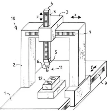
Contact-based techniques require physical contact with the target by a solid object, such as a touch probe. An example of such a system is the coordinate measuring machine (CMM), where a touch probe is used to find and calculate the distance

of each point of a target object. Fig. 1.2 illustrates a CMM. During measurement, component 7 is first moved along they direction. Component 6 (the touch probe) is also moved in both x and z directions. Its location in terms of x, y and z are

Figure 1.1: 3D surface reconstruction techniques.

Non-contact techniques use electromagnetic waves or acoustic waves instead of a solid object. Electromagnetic waves include Gamma-ray, X-ray, visible light and infrared. Acoustic waves include ultrasound. Gamma-ray, X-ray and ultrasound

have short wave-length and can easily penetrate object, they are thus primarily used for inspecting interior structure of an object [3]. Visible light and infrared have median wavelength and cannot normally penetrate object, they are thus used

to reconstruct the outer surface.

(a) (b)

Figure 1.3: LiDAR-based surface reconstruction: (a) Schematic diagram (adapted from [4]) and (b) reconstruction of Rhode Island (adapted from [5]).

1.1.2 Active techniques

Active techniques require the operator or the instrument to provide a source of waves that is used for distant measurement. Popular examples include time-of-flight,

tri-angulation and structured light. In time-of-flight-based techniques, a pulse of laser is emitted onto the target point, reflected by the target and received by a sensor. The time interval for the process is used to calculate the distance. Time-of-flight is

capable of operating over very long range up to 800 metres with 1 centimetre accu-racy [6]. They are thus mainly used for scanning buildings and geographic features

[4]. Light detection and ranging (LiDAR) is a typical example of these techniques. Fig. 1.3(a) illustrates the working principle of an airborne LiDAR carried by an aircraft. The LiDAR constantly scans left and right downwards as the aircraft

recon-struction. Fig. 1.3(b) shows a pseudo-coloured surface reconstruction of the Rhode Island in spring 2011.

In triangulation-based techniques, the light source, the camera and the object

are placed in three different locations, forming a triangle. When the light source is fixed, the position of the reflected light in the image indicates how far the object is from the camera. Triangulation-based techniques provide very high accuracy up to

2.25 micrometres [6]. Applications include inspecting surface defects and precision measurement. Fig. 1.4 illustrates two common types of triangulation techniques,

i.e., the single point laser scanner and the slit laser scanner. The single point scanner shown in (a) works by projecting a single ray of laser onto the object with known orientation. A camera with known configuration and orientation captures

the image of the reflected ray as a sharp point. Finally the depth is computed using the location of the sharp point in the image. This process is repeated many times at

different locations of the target object so that a depth map is obtained. Instead of projecting a single ray, the slit scanner in (b) projects a slit of rays onto the object, which considerably increase the reconstruction speed.

(a) (b)

Figure 1.4: An illustration of the triangulation laser scanner (adapted from [6]): (a) Single point and (b) slit laser scanner.

In structured-light approach, a pattern of light is projected onto the object, and the reflected pattern indicates the distance [7]. Fig. 1.5 illustrates an example of

surface reconstruction using a structured-light technique. Patterns of parallel lines are projected onto the object as shown on the left. Regions with lines having larger

Figure 1.5: Structured-light-based 3D surface reconstruction (adapted from [10]).

is shown on the right by 3D surface rendering. Structured light approach provides

lower accuracy than triangulation, but it is capable of producing smooth surface reconstruction at video rate [6]. Hence, it is ideal for human body measurements where absolute accuracy is not important. Real-time system has been developed,

e.g., Microsoft Kinect sensor which uses infrared as the light source [8]. Stereoscopic systems with structured-light are also commercially available. Two cameras are used

in such a system, the locations of the projected pattern in their field of view are used to calculate distance [9].

1.1.3 Passive techniques

Passive surface reconstruction techniques do not require any active light projection. Instead, the natural radiance, colour and textures of the target surface are used

for distance measurement. Shape from shading and shape from motion are famous examples. Depth from stereo, depth from focus (DfF) and DfD are also passive if no active projection is performed. Shape from shading is based on the fact that

the surface shape affects the reflectance property [11] as illustrated in Fig. 1.6. The reflection distribution, viewing direction and the light source are used as input.

High-quality lighting is required for accurate result. Shape from shading will not work for a random scene where no information is obtained for the light source.

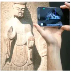
Figure 1.6: Artist’s drawings of 3D shapes (adapted from [12]).

estimate the 3D information. Fig. 1.7 illustrates an implementation of shape from motion on a smart phone, where the orientation and displacement of the camera are obtained with the internal sensors of the camera. Depth from stereo is a

sim-ilar technique, where two images are captured by two cameras at different views. Fig. 1.8(a) illustrates the working principle of a stereoscopic system. Two cameras with known orientation and baseline capture images of an object. The images of

the object points from the two cameras are in different locations. The difference in locations, known as disparity, is larger if the object is closer to the camera. Thus,

disparity is computed to infer depth.

Figure 1.7: An implementation of shape from motion on a smart phone (adapted from [13]).

(a) (b)

Figure 1.8: Depth from stereo: (a) working principle (adapted from [14]) and (b) a commercially available active stereoscopic system (adapted from [15]).

The biggest problem with shape from motion or depth from stereo is finding

point correspondences, i.e. which two pixels correspond to the same object point, and this requires large computational cost and is not always possible. Correspon-dence cannot be found if a point only appears in one of the images but is occluded

Fig. 1.8(b) shows an example of an active stereoscopic system, where a projector projects a pattern of light rays onto the object to aid the correspondence search.

Passive DfF computes distance by analysing camera parameters after the

image is in focus. When the image is in focus, the focal length, and sensor to lens distance are used to calculate depth. The challenge of DfF is in deciding when the object is in focus. Auto focus has become commercially available, but its operational

speed is limited to up to few frames per second. Thus, a dense depth map using DfF is very unlikely to be achieved in real-time.

1.2

Depth from Defocus

In this thesis, depth is the distance from a target object to the viewer, and defocus is the artefact of image blurring. Thus, DfD is a 3D surface reconstruction approach

based on image blurring effect. DfD can take either a single image, two images, or more than two images as its input. Techniques using a single image analyses the frequency content near sharp edges. However, they have an inherent difficulty in

distinguishing whether low frequency regions correspond to blurred sharp edges or focused smooth surfaces. Thus they are primarily used when only one input image is available. Most existing DfD methods use two images as input that effectively

addresses the above-mentioned ambiguity problem. More images can be used which impose over-constraints, thus improving the reconstruction accuracy.

This thesis is concerned with DfD using two images. Fig. 1.9 illustrates the workflow of the DfD approach. First, two images of a scene are captured by a digital camera with different but known focus settings, where focus settings or

optical settings refer to aperture size, sensor to lens distance and focal length. In the top image, the background sandpaper is the furthest object in the scene, and it is

in focus. Thus, this image is called the far-focused image. In the bottom image, the nearest bottom wooden chunk is in focus, this image is thus called the near-focused image.

Far/near-focused image pair is often used as the input to DfD methods, but it is not the only option. Other means of obtaining the image pair include changing

aperture size and focal length. The single-channel (greyscale) image pair obtained by averaging the multi-channel (colour) image pair is used in this thesis as the cases in [16; 17]. A DfD method estimates the depth, pixel by pixel, and generates a

Figure 1.9: Overview of DfD using 2 images.

1.2.1 Mathematical background

Fig. 1.10 shows an image of flowers. It is clear that the flowers which are closer to

the camera are sharper than those further away, or the closer flowers are less blurred than the further ones. This is the basis for DfD, where the amount of blur infers distance. The blurring effect is modelled mathematically as the convolution of the

point spread function (PSF) with a focused image, i.e.

I=H∗M , (1.1)

whereMis the focused image,His the PSF andIis the blurred image. The PSF is associated with a parameter indicating the amount of blurring, which is the defocus

parameter. For example, the Gaussian PSF is given by [18]

H(x, y) = 1 2πσ2e

−x2+y2

2σ2 , (1.2)

whereσ is the standard deviation (SD) or the defocus parameter of the PSF, xand

y are the horizontal and vertical indices respectively. The larger the SD, the more blurred the resulting image becomes. Note also that circular symmetry applies for all PSFs assuming the lens has a non-distorted circular symmetrical shape.

Please also note the mathematical notations used in the thesis: v (lower-case italic letter) denotes a scalar variable, V (upper-case letter) denotes a scalar constant, ~v (arrow overhead) denotes a 1-dimensional (1D) array of elements, V

(bold upper-case) denotes a 2-dimensional (2D) array of elements, matrix or digital image, and ˇV (check overhead) denotes the magnitude frequency response (MFR) ofV.

Fig. 1.11 shows an example of modelling blur with the Gaussian PSF. The first row shows an all-focused image where every pixel in the image is in focus. The

second row shows Gaussian PSFs with SD of 1, 1.3 and 2.5, respectively from left to right. The third row shows the resulting blurred images. As the figure shows, the blurring effect is higher for large value of SD. Hence, when Gaussian PSF is used,

the SD is estimated to obtain depth.

Figure 1.11: An example of blur modelling with Gaussian PSF. Row1: the original image (adapted from [20]). Row 2: surface plot of the PSF with different SD. Row 3: the blurred images.

There are numerous DfD methods. The generic DfD method, i.e., the Sub-barao’s method [18] is based on estimating depth from the amount of defocus, which

is represented by the defocus parameter of PSF. The defocus parameter is computed by solving a system of equations involving input pixel values and optical

parame-ters such as focal length, aperture diameter and sensor-to-lens distance. An outline description of the generic DfD method, i.e., the Subbarao’s method, is presented in Appendix C. Although the generic DfD offers a general clue for estimating depth

and failure to consider the frequency dependency problem, which states that dif-ferent frequency components have difdif-ferent depth responses. In [16], a number of spatial filters, called rational filters or rational operators (ROs) were designed to

address this problem.

Fig. 1.12 illustrates the DfD image acquisition system with telecentric optics1. The light rays from an object point pass through the telecentric aperture of radius

a. The focused image point is tagged at a position between the far-focused position l1 and the near-focused image positionl2. The normalised depthα is -1 atl1 and 1

atl2. The distance between the focused point andl1 is (1 +α)eand that between

the focused point andl2 is (1−α)e. uis the distance between an object point and

the lens andF is the focal length. First, the f-number of the lens

Fe =

F

2a . (1.3)

The optical transfer function (OTF) (please see Appendix C for its definition) of

the frequency-dependant pill-box

ˇ

H(fr, α) =

2Fe

π(1 +α)efr

J1

π(1 +α)e Fe

fr

, (1.4)

where,J1is the first-order Bessel function of the first kind, andfr denotes the radial

frequency.

Figure 1.12: The telecentric DfD system.

1

The normalised image ratio (NIR) or theM/P ratio is given by:

ˇ

M

ˇ

P(fr, α) =

ˇ

H1(fr, α)−Hˇ2(fr, α)

ˇ

H1(fr, α) + ˇH2(fr, α)

, (1.5)

where ˇH1 and ˇH2 are the OTFs of the far-focused and near-focused image, respec-tively. Eqn. (1.5) was modelled as a third order polynomial of the depth α[16],

i.e.,

ˇ

M

ˇ

P(fr, α) =

ˇ

Gp1(fr)

ˇ

Gm1(fr)

α+ Gp2_ˇˇ (fr)

Gm1(fr)

α3 , (1.6)

where the coefficients are expressed as rational forms; ˇGm1, ˇGp1 and ˇGp2 are the

Fourier transform of the ROs.

For offline preparation, Eqn. (1.4) and (1.5) were first used to obtain the NIR. least squares fit was then used to find the first and third order coefficient in

Eqn. (1.6). After ˇGm1 was initialised to be a band-pass filter, the other two filters ˇ

Gp1 and ˇGp2 were computed with the coefficients. The corresponding spatial filters

are denoted by Gm1, Gp1 and Gp2, respectively, which are the rational filters or ROs.

During run-time, the difference imageM and sum image Pwere computed

first using

M= (I2−I1)∗Q (1.7)

P= (I2+I1)∗Q , (1.8)

whereQis a pre-filter that removes the frequency components that degrade surface

reconstruction. DenotingA as the depth map and using Eqn. (1.6),

Gm1∗M= (Gp1∗P)·A+ (Gp2∗P)·A3 , (1.9)

where·denotes the dot product. Solving Eqn. (1.9) gives the depth map.

This DfD method performs detailed analysis on every frequency component

from the input images by obtaining the frequency-variant expression of the OTF and the NIR using Eqn. (1.4) - (1.6). The run-time computation is linear with only 5 convolutions as shown using Eqn. (1.7) - (1.9). Thus, this method is both

accurate and of low computational cost, and it is ideal for real-time 3D surface reconstruction for human activity analysis. In [16], the ROs were designed with a

1.2.2 Motivation

The interest in DfD is motivated by its advantages over other 3D reconstruction

techniques and its potential applications. Contact-based techniques provide mi-crometre precision. However, they are very slow with speed of up to few hundred

object points per second. They are also not suitable for delicate object which might be damaged or modified. Their applications include measurement of the surface of a flat object, and objects with simple curvature in manufacturing industry. Active

techniques provide high accuracy and higher speed than contact-based ones. DfD with structured-light is studied by researchers, where the amount of blurring of the

projected pattern is used to calculate depth. However, active techniques require dedicated hardware, professional calibration and are usually very expensive.

Passive techniques provide considerably lower accuracy than contact-based

active techniques, and thus cannot be used for high precision measurement. How-ever, their implementations are much faster and cheaper since active illumination is

not required. Amongst these techniques, DfD is capable of producing dense depth map with high speed, does not have the correspondence problem associated with depth from stereo since only one view is used, and it can adapt to various lighting

conditions by changing sensor exposure time or aperture diameters. Recently DfD was applied in Panasonic Lumix GH4 digital camera for rapid auto-focus [21], which was significantly faster than traditional DfF-based technique. In contrast with depth

from stereo that requires two lenses, DfD requires only one lens to capture input images, thus it is ideal for applications where the input device needs to be

minia-turised, such as 3D endoscopy. Other potential applications include 3D-modelling, human-computer interaction and human activity analysis where active illumination hardware is not available or practical.

1.2.3 Challenges and contributions

As discussed in Section 1.2.1, the DfD method in [16] is accurate and fast. However,

it suffers the following serious drawbacks that must be addressed. First, it assumes no aberrations or diffraction, and thus uses a pill-box PSF. However, this is not true

for most of the off-the-shelf lenses. Second, the designed pre-filter fails to remove significant amount of frequency components which lead to suboptimal reconstruc-tion. Third, spurious assumptions are made in the unnecessarily complex design

procedure for the ROs. Finally, an elliptical depth distortion resulting from optical lens is not addressed which leads to a distorted depth map.

To address these drawbacks, we propose a DfD system with Gaussian ROs

PSF for the imaging environment when aberrations and diffraction are significant, and the generalised Gaussian ROs with generalised Gaussian PSF2 is applied to the environment with any amount of aberrations and diffraction. Frequency components

containing low gradient along with the zero gradient are removed with the proposed pre-filter. Only one cost function is formed during filter optimisation without the need of any assumption. The elliptical depth distortion is addressed by the proposed

two correction methods: correction by distortion cancellation (CDC) that works by cancelling the distortion with a known similar distortion, and correction by least

squares fit (CLSF) where a mapping from the distorted value to the corrected value at a given location and distance is learnt efficiently by least squares fit.

1.3

Human Activity Recognition

Thus far, a number of common 3D surface reconstruction techniques has been briefly introduced in Section 1.1, and an introduction on the first topic of our thesis, i.e. DfD, has been given in Section 1.2 along with its advantages over the alternative

techniques and its major problems. In this section, an introduction of human activity recognition system that is the second topic of the thesis is provided. The proposed system makes uses of a 3D reconstruction technique to obtain the training data.

Video-based human activity recognition is one of the current most important topic of computer vision research. In recent years, it has attracted the interest of

many researchers from academia, industry, consumer agencies and security agencies. A recognition system aims at the automatic analysis of an activity performed by a person or multiple persons captured in a video or image sequence. In the simplest

case where a video sequence is segmented to contain only a person performing one activity, the system is expected to classify this activity as one of the learnt categories.

There is no consensus terminology for an activity and an action [22]. We thus define an action primitive as a sequence of individual postures of a single body part such as rising arm and kicking. We define an action as a periodic movement

comprising a number of primitives, such as jumping and hand-clapping. We define an activity as a sequence of individual actions that serves a goal, such as walking

while using a mobile phone, and a sequence of digging towards different direction. In this thesis we limit our research to full body of a single human subject using silhouettes. Therefore, recognition of hand gestures and group activities are beyond

the scope of this thesis.

Research in video-based activity recognition is preceded by research in

ob-2

ject recognition and speech recognition before digital video hardware became widely available. Thus, it is significantly inspired by both preceding recognition systems. Systems that are inspired by the former consider a video as a spatio-temporal

vol-ume, which is a 3D volume created by combining the frames from consecutive time instances, and 2D object feature analysis is extended into the 3D case. Examples include a system that incorporates 3D interest points extraction [23] and a system

that uses 3D convolutional neural network (CNN) [24]. Systems inspired by the latter is based on sequential analysis of features extracted from every frame of the

video, and they often use techniques that have been successfully implemented in the speech recognition systems such as the hidden Markov model (HMM) [25] and dynamic time warping (DTW) [26].

The spatio-temporal approach to activity recognition is illustrated in Fig. 1.13. This approach involves a training process and a learning process. The training

in-cludes: generating a spatio-temporal volume from each of a number of videos con-taining different classes of activities; and generating an activity model by extracting features from the volume. During learning, the similarity between different activity

models is defined using measures such as Euclidean distance, Mahalanobis distance and subspace angles. When a video containing an unknown activity is to be

recog-nised, similar processes as in training are performed. A classification algorithm, e.g., nearest-neighbour and Support Vector Machine (SVM), is then performed to label the video as one of the learnt categories based on the defined distance measure.

The sequential approach is illustrated in Fig. 1.14. Raw data such as sil-houettes and body joints are extracted from the video frame by frame. A feature vector is created by extracting features from each frame of raw data, and an activity

model is generated from the feature vectors. Finally the learning and classification procedures are similar to those in the spatio-temporal approach.

Human activities contain complex information and are of high dimension-ality. Thus, there is a need for dimensionality reduction techniques to retain only the discriminating features of human activities. Examples of popular

dimension-ality reduction techniques include principal component analysis (PCA) [28], multi-dimensional scaling [29], locally linear embedding (LLE) [30] and isometric feature

mapping (Isomap) [31].

Fig. 1.15(a) illustrates LLE for feature extraction, where high dimensional images of human faces are embedded into a 2D space. The horizontal dimension is

Figure 1.13: Spatio-temporal approach to human activity recognition (adapted from [27]).

(a)

(b)

set of face images are embedded into a 2D space. The horizontal axis represents left or right pose of the head, and the vertical axis represents up and down pose of the head.

During training, a number of feature vectors are embedded and stored. Dur-ing testDur-ing, a new feature vector needs to be embedded as well in order so as to match it with the stored vectors. Manifold learning involves learning the mapping

from original space to the embedded space. Previous recognition systems made use of linear methods such as PCA [32], where new input vectors could be embedded

by direct projection onto the principal axioms generated by the Singular Value De-composition (SVD) applied to the training data. However, human activity is highly complex and non-linear. A significant improvement was thus made using non-linear

dimensionality reduction methods including Isomap and LLE [33; 34; 35].

1.3.1 Motivation

The interest in human activity recognition is motivated by several important appli-cations, including content-based video analysis, human-machine interaction, patient

monitoring, safety monitoring, and security and surveillance [36]. Content-based video analysis aims to categorise a video according to its contents containing hu-mans performing activities. This has become a very important application for video

sharing websites, which may have the need to automatically assort or evaluate their videos. This is also very important for sport videos [37], such as one containing a football match, where the match statistics require accurate identifications of passing

ball, shooting, and etc.

Human-machine interaction is the mutual action between human and

ma-chine, which involves both input (human to machine) and output (machine to hu-man) communication. Traditional input methods include switching switches, turn-ing knobs, pressturn-ing buttons and typturn-ing with keyboards, and output methods include

acoustic and optical ones. However, these methods are often not intuitive and diffi-cult to learn. Recent success in object recognition and speech recognition has made

it easier for human users to use machine. For example, fingerprint devices have been widely available which save users from typing password, and speech recogni-tion systems allows users to control machines by simply talking to them. Similarly,

activity recognition would encourage users to use machines by performing an action or an activity. However, the required technique for human-machine interaction is

not sufficiently mature and thus it is still an active research area.

patients with chronic disease who need to take medicine regularly for a long period. This is also important for patients in critical conditions who may not be able to contact medical staff. It is inevitable that continuous monitoring of patients leads

to monitoring staff’s physical or mental fatigue, thus an automatic system is highly beneficial for monitoring or surveillance application. Highly hazardous environment can cause injury or death if a dangerous activity is performed, e.g., smoking in

a petrol station and entering a biomedical laboratory without wearing protective clothing. An automatic system that identifies dangerous human activities can

po-tentially reduce such fatal incidents. Traditional security and surveillance systems require a number of video cameras monitored by a human operator. Due to fatigue caused by repetitive nature of the work, abnormal behaviours often go unnoticed.

In addition, with the decrease in the cost of high quality video cameras and the in-crease in the cost of employing human operators, an automatic system that is both

accurate and cost effective has gained a lot of interest from security agencies and other researchers. Another similar application is to automatically identify a target activity from a large video database.

1.3.2 Challenges and contributions

Hitherto, there has been little interest in developing an efficient and accurate means

of obtaining 3D training data for activity recognition [38]. For most recognition sys-tems based on silhouettes, the training data is generated with a camera, or multiple cameras if more views are required. This is impractical if a large number of views are

required, and errors occur in manual camera placement. DfD is potentially useful for this application, where a 3D human body model can be obtained with only two

cameras with one facing another and the subject in between. However, our current DfD system is neither portable nor incorporate real-time automatic input video ac-quisition. Therefore, we propose a method for generating silhouettes from any view

using 3D body coordinates (extracted using Vicon Nexus [39], of each marker placed on an actor while performing an activity) and a triangulation technique for 3D

sur-face reconstruction of the activity. Shadows are inevitably present in real scenes and are difficult to remove reliably from a silhouette [40]. To address this issue we propose a shadow removal method for outdoor scenes based on an estimate of the

current position of the sun and 3D analysis of shadow formation.

Various problems are also encountered by an activity recognition system.

an activity is performed is changed, the template used for its recognition has to be changed as in the space-time volume approach [41; 42]. Real-time operation with high accuracy and robustness are often necessary. However, methods based

on space-time trajectory [43; 44] are very slow because they require accurate 3D modelling of a large number of body parts. They also have problem dealing with occlusion of joints. We address these problems by proposing an embedded pattern

learning (EPL) algorithm which uses a spatial object created from the coordinates of embedded silhouettes to denote an activity. The spatial object takes into account

the speed variation of the actions and is invariant to their temporal order. The algorithm is fast due to its linear nature. Our main contributions on human activity recognition are: (a) a method for generating training silhouettes from a 3D human

model; (b) manifold learning using Isomap [31], where the radial basis function (RBF) learning process is significantly simplified compared to the work in [34]; (c)

a reliable shadow removal method; (d) and EPL for recognising activities.

1.4

Thesis organisation

Chapter 2 and Chapter 3 respectively provide literature reviews on a number of

most important and well-known passive DfD techniques and human activity recog-nition methods. These chapters aim to provide the basic working principles and methodologies of different and state of the art methods.

Chapter 4 presents the experimental procedures for acquiring DfD input images, and this includes a description of the designed hardware and software

en-vironment. Chapter 5 proposes a RO-based DfD (RO-DfD) algorithm using Gaus-sian PSF and generalised GausGaus-sian PSF in order to cope with different amount of lens aberrations and diffraction. This work has been published in [45]. Chapter 6

presents two DfD correction methods which address the elliptical distortion problem in DfD, where experiments are performed on seven objects with four existing DfD

methods to demonstrate their potential in adapting all other DfD methods. This work has been submitted to a journal [46].

Chapter 7 proposes a silhouette generation technique with 3D data obtained

by Vicon Nexus system, which enables efficient acquisition of training silhouettes for any view. Chapter 8 presents a reliable shadow removal technique for outdoor

envi-ronment using known current position of the sun. As more information is obtained from time, location and camera orientation that are used to estimate the length and angle of the shadow, assumptions on colour and texture are not required, and

Literature review on Depth

from defocus

2.1

Introduction

This chapter is split into two sections. The first section is the review on passive DfD

techniques using a single image, which generally compute depth by analysing the frequency contents of the image. The second section reviews the techniques that use two images, which estimate depth maps with more sophisticated approaches

resulting in more accurate results. Individual reviews are arranged in time order with respect to the researcher(s)’s first publication date.

2.2

Depth from Defocus using a Single Image

The first idea of DfD was proposed in [48]. It stated that DfD had two major advantages: it provided similar accuracy to stereo vision while not requiring any correspondence search; unlike DfF, the best focus point location was not required.

In [49], two DfD methods were presented. One of them used Gaussian PSF and the sharp discontinuities (edges) in a single defocused image to recover depth. First the

edges were analysed within every local region by a Laplacian filter. As a result, the SDσ of the PSF was obtained. The final estimate of the depth was given by

u= F s s−F −σFe

, (2.1)

whereF is the focal length,s is the sensor to lens distance andFe is the f-number

of the lens. To produce a dense depth map with high resolution, each of the input

depth value within one region was assumed to be the same and was then computed. This process is repeated for all regions to obtain the depth map. In this thesis, we use the term “local image region”, “patch”, “window” and “neighbourhood”

interchangeably. Experiments with a real image showed that the depths of the region near the sharp edges were recovered. The edges could be categorised into high, medium and low in terms of depth. However, a complete depth map could not

be computed with this method.

In [50], a simplified version of the method in [49] was presented. A term

called “spread parameter”σlwas introduced, which indicated the defocus degree of

an edge. Hence it is a 1D analogue to the SD σ of the Gaussian PSF. The depth was found with an equation which related σl and camera parameters to depth.

Experiments were performed with a cardboard paper, the surface of which was drawn with black and white strips. Higher accuracy was achieved for objects closer

to the camera than further ones. The working distance was reported to be about 8 feet.

In [51], the method using a single image in [49] was generalised. The edge

orientation that was important for [49] was not required. In addition, a new method was developed to estimate the SD of the PSF so that the approach was less sensitive

to noise disturbance. An average error rate of 5% was reported using real images. This approach could be applied to both step edges and ramp edges. However, the computational cost was high for ramp edges.

Also based on the work in [49], a DfD method was proposed in [52] using moment preservation and proportion of edge pixels in local regions. The image sensor was pre-adjusted to be behind the nearest focused points, thus only one

image was required. A gradient image was then obtained using a Sobel filter. The diameter of the blur circle used to determine depth was found proportional to the

edge pixels in a corresponding local region in this gradient image, which was used to calculate depth. The first three moments of the local region were then computed in terms of the proportion of the diameter and the local region. Therefore the

proportion could be determined which in turn determines the depth. Furthermore, an artificial neural network (ANN) was used to deal with optical errors. However,

the method required a circular local region with a radius of 35 pixels, which would only provide a limited depth resolution.

A DfD method using endoscopic video was proposed in [53]. Traditional

DfD methods captured one or two images of the target scene at the same view. In contrast, this method used multiple images from different views with frames from

Laplacian filtering and Sobel filtering. By assuming the location of the camera was known during recording, a complete 3D model was then reconstructed from all the edge depth maps using triangulation.

In [54], a conventional camera was modified by placing a coded aperture in front of the lens (see Fig. 2.1) to achieve better performance. Fig. 2.2 illustrates the working principle using a PSF at 3 different scales and the corresponding frequency

domain representation.

(a) (b)

Figure 2.1: Coded aperture illustration adapted from [54]. Left: a coded aperture placed in front of the lens; right: the resulting blur pattern.

Figure 2.2: PSFs at different scales and their frequency response adapted from [54].

The idea behind the method is to consider the zero-crossing of the frequency.

For example, f1 is less blurred compared to f2, therefore the zero-crossing ω1 is

larger thanω2. In other words, the scale in the frequency domain infers depth. The

probability distributions of the focused image and blurred image at different scales

were formulated with the zero-crossing idea. For aperture design, the Kullback-Leibler divergence was maximised for the distributions of the PSF at different scales

thus providing higher distinguishability. The focused image was found first by max-imising a probability distribution model. The depth was then estimated in closed form. As a result, a layered depth map was formed as shown in Fig. 2.3.

(a) (b)

Figure 2.3: An illustration of the layered depth map from [54]. Left: original image; right: layered depth map.

of various scenes and the corresponding depth maps obtained from a laser scanner. It argued that local feature alone was not sufficient to estimate depth, and the global

context should have also been considered. Thus, a hierarchical Markov random field (MRF) was used to find the depth relationship between different points in the image. The MRF [56] is an undirected graph (e.g., an image or a depth map) of random

variables having the Markov property, i.e., in the depth estimation case the blur operation in a local region depends on its adjacent regions. An average root mean

square error (RMSE) of 0.09 on log scale was obtained. Although the performance of this approach was lower than earlier DfD methods such as [50] and [51], the target scenes were much more complex and the input images were obtained from

uncontrolled environment. The computing speed was not given, but the complex nature of the approach implies it is unlikely to be a fast algorithm.

In [57], the input image was re-blurred using a Gaussian kernel. The amount of blur near the sharp edges was estimated from the ratio between original image and the re-blurred image. As a result, a defocus map for all sharp edges was acquired.

By interpolating the edge defocus map in 3D space, a defocus map was obtained. A full depth map was estimated from the defocus map with camera parameters. The results demonstrated that high definition defocus maps could be obtained with low

computational cost.

2.3

Depth from Defocus using Two Images

We group these approaches into five categories. First, Fourier domain approach

extracts the defocus parameter with Fourier transform of the input images. Second, spatial-filtering approach computes depth by convolving the input image with digital

The general procedure comprises three stages: a statistical model is first applied to the focused image and the depth map; an estimator/cost function is then formulated with its property, with the arguments being the focused image and the defocus

parameter or depth; finally the result is obtained by optimising the estimator/cost function iteratively. Fourth, machine learning approach stores a number of patterns and their corresponding depth values. When an input patch is given, it matches

with the stored library to determine depth. Fifth, other approaches that do not fall into any of the above four categories.

2.3.1 Fourier domain approach

One of the methods in [49] estimated depth using two images at the same view,

one of which was captured with a pin-hole camera. Gaussian PSF was used and its SD was computed first. The image captured from an ideal pin-hole camera was all focused. The SD was thus zero throughout the image. Fourier transform was

performed for a small local region in both images. As a result, the SD of the second image was obtained. This method could be implemented efficiently with fast Fourier

transform (FFT). Experiments showed that the accuracy was comparable to that achieved by depth from stereo or depth from motion.

The DfD method in [18] generalised the method in [49] which required one

image to be captured with a pin-hole camera. The two images could be captured with any different set of camera parameters, including aperture size, sensor-to-lens distance and focal length. Gaussian PSF was used and its SD was used to calculate

depth. The SD was expressed in terms of the camera parameters and depth. Every local region in the image pairs were converted to the frequency domain by Fourier

transform. The depth was estimated within the frequency domain. This method was considerably more accurate than that in [49] and [58] when sensor-to-lens distance was varied to obtain the input images, which avoided the noise associated with using

a pin-hole camera set-up.

The method in [59] was based on 1D Fourier transform instead of 2D Fourier

transform as in [18]. 1D Fourier transform is faster to compute than the 2D Fourier transform, and it is also robust in the presence of zero-mean noise. First the two input image-patches were summed row-wise to obtain two 1D sequences, which were

then normalised with respect to brightness. The first 6 discrete Fourier coefficients were then used to create a computed table that corresponds to a specific depth.

This table was created in a lookup table fashion which was searched during run-time depth estimation. Experiments showed a 6% error.

re-gression fit in the frequency domain of every local region in order to calculate the defocus parameter, and thus was not well suited to the optical system. Instead, the entropy concept was applied to overcome this problem. As entropy is a measure of

information content, a blurred image has less entropy than its focused version. It was used to derive the defocus parameter as a function of the input images without regression. The experiments showed that the method outperformed the method in

[49]. However, one of the input images was still obtained by a pin-hole camera. The method in [61; 62] argued that previous DfD methods assumed the depth

to be constant over fairly large local region, and considered the blurring to be shift-invariant over those local regions, which leaded to errors when the neighbourhood regions were not considered. This problem occurred since the blurred image could

not be simply modelled as the convolution between a shift-invariant PSF and the focused image due to the blurring from the neighbourhood pixels. Two methods

were proposed to address this problem. The first method modelled the DfD system as block shift-variant, where the PSF incorporated the interaction of the blur from the surrounding regions. The second method was based on the space-frequency

representation of the local regions. The space-frequency representation is the exten-sion of time-frequency representation [63] in image domain. The Short-time Fourier

transform and the Wigner distribution are famous examples of time-frequency rep-resentation. The second method applied the space-frequency representation of the local region instead of the Fourier transform to allow the blur operation to be

shift-variant. An experiment on simulated image compared these two methods with the one in [18]. It showed that the RMSE of these two methods and [18] are 47%, 14% and 6%, respectively. Experiments were also performed on real images with the

object placed between 90 and 120 cm away from the camera, which showed that the RMSEs of these two methods were 7.43 cm and 6.18 cm, respectively.

The windowing effect is an artefact produced during Fourier transform of the local image regions, or windows. This leads to spurious high-frequency components at the region boundary. Xiong and Shafer [64] proposed moment filters to address

the windowing effect. Gaussian PSF was used but the method was claimed to be applicable to any model. The moment filters were expressed as a function of

exponential function whose coefficient was the generalised Laguerre’s polynomial. Thenth moment could be thought ofnth derivative of the Gaussian PSF, hence the filters were used to replace the single first order Gaussian PSF. By a complex analysis

in frequency domain, an equation was derived for estimating the defocus parameter. They reported that the finite window problem and the shift variance problem were