warwick.ac.uk/lib-publications
Original citation:
Jiang, Jing, Dianati, Mehrdad, Imran, Muhammad Ali, Tafazolli, Rahim and Zhang, Shunqing. (2014) Energy-efficiency analysis and optimization for virtual-MIMO systems. IEEE
Transactions on Vehicular Technology, 63 (5). pp. 2272-2283.
Permanent WRAP URL:
http://wrap.warwick.ac.uk/90551
Copyright and reuse:
The Warwick Research Archive Portal (WRAP) makes this work by researchers of the University of Warwick available open access under the following conditions. Copyright © and all moral rights to the version of the paper presented here belong to the individual author(s) and/or other copyright owners. To the extent reasonable and practicable the material made available in WRAP has been checked for eligibility before being made available.
Copies of full items can be used for personal research or study, educational, or not-for profit purposes without prior permission or charge. Provided that the authors, title and full bibliographic details are credited, a hyperlink and/or URL is given for the original metadata page and the content is not changed in any way.
Publisher’s statement:
© 2014 IEEE. Personal use of this material is permitted. Permission from IEEE must be obtained for all other uses, in any current or future media, including reprinting
/republishing this material for advertising or promotional purposes, creating new collective works, for resale or redistribution to servers or lists, or reuse of any copyrighted component of this work in other works.
A note on versions:
The version presented here may differ from the published version or, version of record, if you wish to cite this item you are advised to consult the publisher’s version. Please see the ‘permanent WRAP url’ above for details on accessing the published version and note that access may require a subscription.
Energy Efficiency Analysis and Optimization
for Virtual-MIMO Systems
Jing Jiang,
Member, IEEE,
Mehrdad Dianati,
Member, IEEE,
Muhammad Ali Imran,
Senior Member, IEEE,
Rahim Tafazolli,
Senior Member, IEEE,
Shunqing Zhang,
Member, IEEE.
Abstract
A virtual multiple-input multiple-output (MIMO) system using multiple antennas at the transmitter
and a single antenna at each of the receivers, has recently emerged as an alternative to a
point-to-point MIMO system. This paper investigates the relation between energy efficiency (EE) and spectral
efficiency (SE) for the virtual-MIMO system that has one destination and one relay using
compress-and-forward cooperation. To capture the cost of cooperation, the power allocation (between the transmitter
and the relay) and the bandwidth allocation (between the data and cooperation channels) are studied.
This paper proposes a novel and tight upper bound for the overall system EE as a function of SE, which
exhibits a good accuracy for a wide range of SE values. The EE upper bound is used for formulating
an EE optimization problem. Given a target SE, the optimal power and bandwidth allocation can be
derived such that the overall EE is maximized. Results indicate that EE performance of virtual-MIMO
is sensitive to many factors including resource allocation schemes and channel characteristics. When
an out-of-band cooperation channel is considered, virtual-MIMO performs close to the MIMO case
in terms of EE. Considering the shared-band cooperation channel, the virtual-MIMO with the optimal
power and bandwidth allocation is more energy efficient than the non-cooperation case under most SE
values.
Index Terms
Energy efficiency, Virtual MIMO system, CF cooperation, Power allocation, Fading channels.
J. Jiang, M. Dianati, M. A. Imran and R. Tafazolli are with the Centre for Communication Systems Research, Depart-ment of Electronic Engineering, University of Surrey, GU2 7XH, Surrey, U.K. (Email: {Jing.Jiang, M.Dianati, M.Imran, R.Tafazolli}@surrey.ac.uk)
I. INTRODUCTION
Virtual multiple-input multiple-output (MIMO) systems, where the transmitter has multiple
antennas and each of the receivers has a single antenna, have recently emerged as an effective
technique that can improve spectral efficiency of wireless communications [1] [2]. The idea is
that when channel state information (CSI) is available at the receiver side only, some
neigh-bor receivers can contribute their antennas (i.e., serve as relays) and help the single-antenna
destination to form a virtual antenna array and to reap some benefits of MIMO systems [3],
[4]. Virtual-MIMO is a promising idea for terrestrial mobile communication systems as some
mobile stations in these systems may not be equipped with multiple antennas due to the physical
constraints.
Most of the previous work on virtual-MIMO systems focused on spectral efficiency (SE)
and bit error ratio performance, such as [2], [4], and [5]. It was shown that the cooperation
among receivers could enhance the efficiency of frequency spectrum utilized, compared to the
non-cooperative multiple-input and single-output (MISO) systems. However, the SE metric fails
to provide any insight on how efficiently the energy is consumed. The impact of cooperation,
considering a realistic model that takes into account both transmit and circuit energy consumption
at the transmitter and relay nodes, on the overall energy efficiency (EE) of the system has not
yet been adequately studied, to the best of our knowledge. In addition, maximizing the EE,
or equivalently minimizing the total consumed energy, while maximizing the SE are generally
conflicting objectives; but they can be linked together and balanced through their relationship
[6]. That is, for certain values of SE, whether and under what conditions the cooperation at
the receiver side can offer benefits in terms of overall EE, when a realistic energy
consump-tion model is considered. This is particularly an important quesconsump-tion for network operators and
telecommunication equipment manufacturers as there is a global demand for the future wireless
networks to become more energy efficient [7]–[9].
Essentially virtual-MIMO can be viewed as a combination of MIMO and cooperation
technolo-gies. From the cooperation perspective, the relay node in virtual-MIMO systems can use either
EE performance of these relay protocols have been studied in [10]–[12], where a classical relay
channel (with three single-antenna nodes) is considered. In [10] and [11], a linear approximation
of the EE-SE trade-off is derived for relay communications by using the first and second
derivatives of the channel capacity. This study is then extended in [12] where the synchronization
between the transmitter and the relay are considered for practical scenarios. The approximation
of the EE-SE trade-off in these previous papers is accurate in the low SE region but largely
inaccurate otherwise. In addition, the aforementioned papers do not take circuit energy into
consideration, which may not be negligible in practical wireless networks [8]. A more accurate
approximation on the EE-SE trade-off for MIMO Rayleigh fading channels is presented in [6]:
The approximation is in closed form, but the expression cannot be extended to a cooperative
virtual-MIMO scheme. An initial study of virtual-MIMO based cooperative communications
for distributed wireless sensor networks is given in [13], where the energy consumption of a
traditional MIMO system and that of a virtual-MIMO scheme are evaluated. This work is then
extended in [14] by taking into account the properties of propagation environment and the energy
overhead required for channel estimation. The corresponding energy consumption assessments
of virtual-MIMO systems in [13] and [14] are based on numerical results and applicable for the
specific configurations considered in these papers.
An important open problem in virtual-MIMO communications is to obtain a general analytic
formula for EE as a function of SE, and use it to identify the potential ways to improve EE.
However, calculations of the system ergodic capacity in Rayleigh fading channels require taking
expectations with respect to a random channel matrix. In general, the problem of defining an
explicit expression to link EE and SE requires an expression for the inverse function of the
capacity, and therefore is a mathematically challenging task. In this paper, we propose a novel
and accurate upper bound of EE as a function of SE for a virtual-MIMO system using the
receiver-side cooperation with the CF protocol. To get a full picture of the overall EE for the
system, both transmit energy and circuit energy consumed at the transmitter and relay nodes are
taken into account. A comparison among different relay protocols in terms of EE is also given
• We analyze the relation between EE and SE for the virtual-MIMO system where a realistic
power model is considered. To this end, we derive a tight closed-form upper bound for the
ergodic capacity of the system, based on which we propose a novel upper bound for EE as
a function of SE which exhibits a good accuracy for a wide range of SE values. The EE
upper bound is used for assessing the EE ratios of virtual-MIMO over the ideal MIMO or
the non-cooperative MISO system.
• We formulate an EE optimization problem based on the EE upper bound. Given a target SE,
the optimal power allocation (between the transmitter and the relay) and optimal bandwidth
allocation (between the data and cooperation channels) are derived such that the overall
EE is maximized. The optimal solution for power allocation is obtained in a closed-form
expression when out-of-band cooperation channel is used.
• To capture the cost of cooperation, we place power constraints in the system, and investigate
different bandwidth allocation scenarios for the data and cooperation channels. We show
that EE performance of virtual-MIMO is close to MIMO when an out-of-band cooperation
channel is considered. Taking the shared-band cooperation channel into account, the
virtual-MIMO with equal bandwidth allocation is less energy efficient than MISO; but with optimal
power and bandwidth allocation, virtual-MIMO outperforms MISO in terms of EE under
most values of SE.
The rest of this paper is organized as follows. Section II describes the channel model and the
realistic power model. Section III evaluates the relation between EE and SE of virtual-MIMO,
including deriving an accurate upper bound of EE in Section III-B. EE optimization issues are
investigated in Section IV. Simulation results are in Section V, and Section VI concludes the
paper.
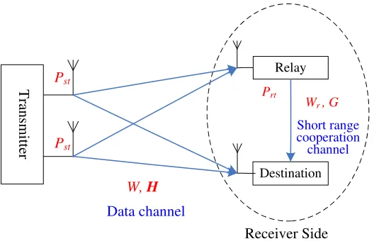
II. SYSTEMMODEL
We consider a transmitter node withNtantennas and a destination node with a single antenna,
as shown in Fig. 1. There areNr−1single-antenna relays in the proximity of the destination. We
a virtual-MIMO system [4]. We assume that the nodes within the receiver group are close, but the
distance between the transmitter and the receiver group is large. For the sake of demonstrating
performance of EE with more tractable mathematical expressions, we consider Nt=Nr = 2
in this paper. Further performance improvements are expected for the case of more transmit
antennas and more cooperating terminals. There are two orthogonal communication channels:
the data channel between the transmitter and the receiver group, and the cooperation channel
between the receivers.
A. Channel Model
In Fig. 1,x= [x1, x2]T denotes the transmitted signals, and[yr, yd]T denotes the corresponding
received signals at the relay and the destination. Without loss of generality, the data channels are
represented byhi=
ci
√
Ktdζ/2
(i∈[1, ...,4]), where ci is a circularly symmetric complex Gaussian
random variable with unit variance and zero mean. As the relay is close to the destination, we
assume that they are equally distanced from the transmitter, which is denoted by d. The scalar
ζ is the path loss exponent, and Kt is a constant indicating the physical characteristics of the
channel and the power amplifier [15]. That is, the data channels are modeled as Rayleigh fading
with E[|hi|2] = 1/(Ktdζ). In matrix form, the received signal vector is
yr
yd
=Hx+n; H=
h1 h2
h3 h4
, (1)
where the data channel matrix H ∈ CNr×Nt is complex Gaussian distributed. n= [n
1, n2]T is
the noise vector with components n1, n2∼CN(0, N0). We assume that perfect CSI is available
at the receiver side only. Let W denote the bandwidth of the data channel. And suppose that
the two antennas at the transmitter use the same average transmit power Pst, i.e., E[|x1|2] =
E[|x2|2] =Pst. Here we consider equal power allocation among the transmit antennas as it is an
optimal power allocation when no CSI is available at the transmitter side [16].
At the receiver group side, there is a short-range cooperation channel between the relay and the
channel to the power gain of data channels is represented by G. As the receivers are closer in
our system model, the case of interest is when G is high. Wr and Prt denote the bandwidth of
the cooperation channel and the transmit power of the relay, respectively.
B. Realistic Energy Consumption
In a practical setting, to quantify the total energy consumption of the entire system, both
the transmit energy and circuit energy consumed at the transmitter and the relay need to be
considered. For instance in [8] and [17], the total supply energy at a base station includes the
energy consumed for the power amplifier, radio frequency circuitry, baseband unit, direct current
(DC)-DC and alternating current (AC)-DC converters. In general, the total supply power and the
transmit power at a base station is nearly linear and, consequently, a linear power model has
been defined in [8] and adopted in this paper. Therefore at the transmitter, the total power for
Nt antennas is given by Nt(ξsPst+Psc), where Psc is the load-independent circuit power at the
minimum nearly-zero output power, and ξs is the scaling factor of the load-dependent power.
For the relay, using a similar linear power model, we have the total supply power(ξrPrt+Prc),
where Prc denotes the load-independent circuit power at the relay. Note that the scaling over
signal load (i.e. the values of ξs andξr) largely depends on the type of the station. Table 2 in [8]
presents the model parameters for various transmitter types in a 3GPP LTE network, and Table
I in [18] presents the parameters for the relay model, which could be adopted in our system.
We assume that the transmitter and the relay are subject to separate power constraints: 0 <
Pst ≤ Pmax,s and 0 < Prt ≤ Pmax,r. For the relay, we define γ = Prt/Pst to be the power
allocation ratio between the relay and the transmitter. Compared to a total power constraint, this
assumption of separate power constraints is more practical for wireless networks, because the
transmitter and relay are usually geographically separated and are supported by separate power
choosing a value of γ). Finally, the total power of the entire system is
Ptot=Nt(ξsPst +Psc) +ξrPrt+Prc = (Ntξs+γξr)Pst+NtPsc+Prc;
0< Pst ≤Pmax,s, 0< γ ≤Pmax,r/Pst.
(2)
C. Impact of Relay Protocol
Relay protocols are usually classified into three categories: DF, AF, and CF, which require
different signal processing techniques at the relay. But these techniques have a similar complexity.
Since the power consumed in the baseband unit is mainly defined by the complexity, the power
difference of the three protocols (caused by different signal processing techniques) is quite small
compared with other parts of the circuit power (such as that for the radio frequency circuitry),
and can be neglected. We thus consider the circuit power at the relay Prc remains the same
for the three relay protocols. In addition, the relay is assumed to be closer to the destination in
this paper; compared to DF, the CF protocol provides superior capacity performance [5], [20].
Therefore, given the same Prt, DF and CF have the same total power consumption; but CF is
more spectrally efficient. According to the definition of EE, CF has a better EE than DF.
In addition, the AF protocol is a special case of CF, in which case the relay simply scales and
forwards the analog signal waveform that is received from the transmitter without any particular
processing [21]. AF requires equal bandwidth allocation for the data and cooperation channels, as
the amplified analog signal needs to occupy an unchanged bandwidth. But, for CF, the signal at
the relay is quantized and can be re-encoded, so that the bandwidth of the cooperation channel
can be changed and optimized as will be shown in Section IV-B. Therefore, for any given
channel conditions, CF performs better than or equal to AF in terms of their EE performance.
Thus in this paper, we assume the relay sends its observation to the destination implementing
CF cooperation, where a standard source coding technique [5] is used by the relay.
III. SPECTRALEFFICIENCY ANDENERGYEFFICIENCY OF THEVIRTUAL-MIMO SYSTEM
In this section, we evaluate the relation between EE and SE of the virtual-MIMO system. We
explicit and accurate approximation of the EE as a function of SE is derived, and is utilized for
assessing analytically the EE gain or loss of virtual-MIMO over the MISO or MIMO systems.
A. Ergodic Capacity of Virtual-MIMO: Explicit Expression VS. Upper Bound
The system model that specified in Section II can be considered as a system where the
destination has two antennas that receive the signals [yr +nc, yd]T [20]. Here nc ∼ CN(0, σc2)
is the compression noise, which results from the CF protocol. As we employ a standard source
coding technique to implement the CF protocol at the relay, we denote Rc as the source coding
rate at the relay which is (smaller than but arbitrarily close to) [2], [22]
Rc =Wrlog2
1 + G
Ktdζ
· Prt
N0Wr
. (3)
Then the variance of the compression noise nc is [2]
σc2 = E[|yr|
2]
2Rc/W −1 =
(|h1|2+|h2|2)Pst+N0W
1 + G
Ktdζ
· Prt
N0Wr
Wr/W
−1
. (4)
The value of σ2
c is related to Rc, and thus determined by channel conditions and energy
consumption. The destination scalesyr+nc using the degradation factorη, such that√η(yr+nc)
and yd have the same power of additive Gaussian noise [5]; thus
˜
y= [√η(yr+nc), yd]T =Hxe + [˜n1, n2]T; He ∆
=
√
ηh1 √ηh2
h3 h4
; η=∆ N0NW0W+σ2 c
, (5)
where ˜n1 ∼ i.i.d. CN(0, N0). In (4), if |h1|2+|h2|2 could be replaced by its expected value, η
in (5) would become constant given certain average channel condition and energy consumption,
and therefore the scaled channel He would be a complex Gaussian matrix. The numerical results
in [4] have demonstrated the accuracy of this replacement. Thus it is reasonably appropriate
corresponding capacity evaluation. Then from (4) and (5), we have
¯
η=
1 + G
Ktdζ
· γPst
N0Wr
Wr/W
−1
1 + G
Ktdζ
· γPst
N0Wr
Wr/W
+ 2Pst (KtdζN0W)
, (6)
and He ∼ CNNr,Nt(0,Ψ⊗I). Ψ is the covariance matrix
Ψ=E
√ ¯ ηh1 h3
√ηh¯ 1 h3
= ¯
η/(Ktdζ) 0
0 1/(Ktdζ)
. (7)
Then Ξ = HeHe† has a complex central Wishart distribution with Nt degrees of freedom and
covariance matrix Ψ, i.e. Ξ ∼ CWNr(Nt,Ψ). Here Nt ≥ Nr is considered. In the following
lemma, we give a result on the complex central Wishart matrix.
Lemma 1: If Y ∼ CWNr(Nt,Ψ), then we have
E[det(Y)] = det(Ψ)
NYr−1
j=0
(Nt−j). (8)
The proof of Lemma 1 is given in Appendix A.
With the CF protocol, the ergodic capacity of the virtual-MIMO system is given by [5], [22]
CCF =E
Wlog2det
I+ Pst
N0W
Ξ
bits/s. (9)
The following result gives a upper bound for the explicit expression of ergodic capacity when
signal-to-noise ratio (SNR) is not low.
Proposition 1: If He ∼ CNNr,Nt(0,Ψ⊗I), i.e. for the considered virtual-MIMO system with
CF cooperation, when SNR is not low, the ergodic capacity upper bound CbCF is
b
CCF=W
Nrlog2
Pst
N0W
+ log2
Nt!
(Nt−Nr)!
+ log2det(Ψ)
bits/s. (10)
The proof of Proposition 1 is given in Appendix B. This proposition provides a simple and
but has the advantage of being express in a closed form and can be used to evaluate the relation
between EE and SE for the virtual-MIMO system.
B. Upper Bound on Energy Efficiency
We use the well known definition of the system achievable EE as the number of bits transmitted
per Joule of energy, i.e. ECF =CCF/Ptot in bits/Joule. According to equations (2) and (9), both
Ptot and CCF are related to the transmit power Pst. Thus the impact of CCF on ECF can be
expressed as follows
ECF =CCF
(Ntξs+γξr)f−1(CCF) +NtPsc+Prc
−1
, (11)
where f−1: CCF 7→ Pst is the inverse function of CCF. Equation (11) indicates that obtaining
an explicit expression ofECF boils down to finding an explicit formula forf−1(CCF). However,
due to the random Rayleigh channel realizations, f−1(CCF) does not have a straightforward
formulation. One feasible approach would be to use the closed-form upper bound of CCF in
(10) for finding an explicit solution to f−1(C
CF). This approach will help us obtain a EE upper
bound as a function of SE, which can be used for explicitly tracking the EE performance and
analytically assessing the EE optimizations for a given SE, and thus will be discussed in this
subsection.
We use SCF to denote SE of the system. Two scenarios of the bandwidth allocation between
the data channel and the cooperation channel are considered in this paper: Scenario I, the relay
uses out-of-band channel for cooperation; Scenario II, the relay uses a portion of the whole
channel. In Scenario I, we assume the data channel and the out-of-band cooperation channel
have equal bandwidth, i.e. Wr = W. As suggested in [2], this is applicable when the separate
band used for short-range cooperation can be spatially reused across all other cooperating nodes
in a network and hence the bandwidth cost for a particular cooperating pair can be neglected
here. In Scenario II, a single channel is divided into two different bands to implement the
cooperation. Scenario II is applicable when spatial reuse of cooperation bands is not considered,
the bandwidth allocation, we define φ = Wr/W. Therefore, we have SCF(ECF) = CCFW(Pst) for
bandwidth Scenario I, and SCF(ECF) =
CCF(Pst)
W+Wr for bandwidth Scenario II. The choice of SCF
and CCF differentiates SE and system capacity, and also helps avoid the abuse of notations that
correspond to the functions of ECF and Pst [12].
1) Bandwidth Scenario I:
For Scenario I, when W=Wr, (6) is further simplified
¯
η = GγPst
KtdζN0W +GγPst+ 2Pst
. (12)
Inserting (12) in (7), and from (10), we have
b
CCF=W
2 log2
Pst
KtdζN0W
+ 1 + log2
GγPst
KtdζN0W +GγPst+ 2Pst
bits/s. (13)
According to the definition of EE, we can obtain a closed-form upper bound for the system EE
as shown in the following.
Proposition 2: Consider the virtual-MIMO system with CF cooperation. For Scenario I, the
upper bound for the number of bits transmitted per Joule of energy, denoted by EbCF, is
b
ECF =W SCF
"
(2ξs+γξr)2
SCF
2 − 1
2KtdζN0W
s
Gγ+ 2
Gγ + 2Psc+Prc #−1
,
with SCF≤2 log2
Pmax,s/(KtdζN0W)
+ 1 + log2[Gγ/(Gγ+ 2)]. (14)
The proof of Proposition 2 is given in Appendix C.
For Scenario I, the EE upper bound EbCF is obtained in closed form, and thus the relation
between EE and SE is explicit. The closed-form EE upper bound and its application environment
(i.e. Scenario I) are particularly valuable and attractive to some realistic wireless communication
systems. For example, the closely located relay and destination could perform cooperation
through their out-of-band Wi-Fi without sharing the frequency bands for data channel that uses
3G (or 4G) cellular communications.
In addition, as shown in (14), Psc and Prc are the load-independent circuit power at the
Psc and Prc dominate the EE performance, and thus ECF is very low. With SCF increasing, ECF
increases but will finally decrease. Therefore, compared to the case without considering circuit
energy consumption, there is no longer a monotonic trade-off relationship between EE and SE
for this system. There exists a certain region of SE that corresponds to a better EE performance,
as will shown in Section V.
2) Bandwidth Scenario II:
We now consider a single channel to be divided into two different bands to implement the
cooperation, and demonstrate its impact on the EE analysis. Using φ=Wr/W, (6) is shown as
¯
η= N0W Ktd
ζ+GγP st/φ
φ
−N0W Ktdζ
(N0W Ktdζ+GγPst/φ) φ
+ 2Pst
. (15)
Inserting (15) in (7), and from (10), we have
b
CCF =W
"
2 log2
Pst
KtdζN0W
+ 1 + log2 N0W Ktd
ζ +GγP st/φ
φ
−N0W Ktdζ
(N0W Ktdζ+GγPst/φ)φ+ 2Pst
!# .
(16)
Different from (13), we cannot get a closed-form solution for Pst from (16) because of φ. To
give an explicit relationship between EE and SE under this scenario, we represent the solution
of (16) as follows
Pst =f−1(CbCF) =KtdζN0W · RP
(
2SCF(1+φ)−2P2 (1 +GγP /φ)
φ−
1
(1 +GγP /φ)φ+ 2P )
, (17)
whereP =Pst/(N0W Ktdζ), and the functionRP{g(P)}denotes the exact roots of the equation
g(P) = 0 with respect to its single variable P. Note that one can apply differentiation or partial
differentiation to RP{g(P)}. Substituting (17) into (11), and let SCF = (1+CφCF)W, we thus obtain
a EE upper bound for Scenario II as shown in the following.
Proposition 3: Consider the virtual-MIMO system with CF cooperation. For Scenario II, the
upper bound for the amount of bits transmitted per Joule of energy can be represented as
b ECF=
SCF/(KtdζN0)
2Psc+Prc
KtdζN0W + (2ξs+γξr)· RP
n
2SCF(1+φ)−2P2 (1+GγP /φ)
φ−1
(1+GγP /φ)φ+2P
HereSCF is also restricted by Pmax,s; Replacing Pst by Pmax,s in (16) gives the constraint on SCF.
Given some values ofφ, the roots RP{g(P)}can be represented in closed form. Takingφ = 1
for example, i.e. Wr =W, we have
RP
(
2SCF(1+φ)−2P2 (1+GγP /φ)
φ−
1
(1+GγP /φ)φ+2P )
≈ RP
22SCF−2P
2Gγ
Gγ+2
= 2SCF s
Gγ+ 2
2Gγ . (19)
Inserting (19) to (18), the closed-form EE upper bound for Scenario II is obtained. For some
other values of φ, if the roots cannot be represented in a simple form, one can use Newton’s
method to find approximations to the roots. The EE upper bound in Proposition 3 removes
the effects of random channel variations, and thus can be used for explicitly tracking the EE
performance of virtual-MIMO, and analytically assessing the EE gain or loss of virtual-MIMO
over the MISO or MIMO system.
3) On Energy Efficiency Comparisons:
The EE upper bound of the ideal MIMO system (as if the receivers were connected via a
wire) and that of the non-cooperative MISO system (where the relay is silent) are given by
b
EMIMO =
W SMIMO
2Psc+ξs2
SMIMO−1
2 KtdζN0W
, where SMIMO ≤2 log2
Pmax,s/(KtdζN0W)
+ 1; (20)
b EMISO =
W SMISO
2Psc+ξs(2SMISO−1)KtdζN0W
, where SMISO ≤log2
1 +Pmax,s/(KtdζN0W)
.
(21)
To obtain (20), we solve Pst from (10) where the covariance matrixΨ =I for the ideal MIMO
case. Then substituting the solution of Pst into the EE expression EMIMO = Nt(W SPscMIMO+ξsPst), and
considering the power constraint 0 < Pst ≤ Pmax,s, we thus obtain (20). In a similar way, but
taking into account Nt = 2 and Nr= 1, we get (21) for the MISO case.
In order to evaluate how virtual-MIMO compared with MIMO and MISO systems in terms of
EE, we use the EE ratios EMIMO/ECF and EMISO/ECF. For a certain value of SE, the EE ratios
boil down to the total power ratios of the corresponding systems. We first consider bandwidth
in the low and high-SE regimes, respectively, can be approximated as
lim
SE→0
EMIMO
ECF
= 2Psc+Prc 2Psc
; lim SE→∞ EMIMO ECF ≈ lim SE→∞ b EMIMO b ECF = s
Gγ+ 2
Gγ ·
2ξs+γξr
2ξs
. (22)
In the low SE regime, the load-independent circuit power dominates the EE ratios. With SE
increasing (when no SE constraint is considered), the ratio of EMIMO/ECF finally approaches a
constant value, as will be illustrated in Section V. Similarly, the theoretical EE ratios of MISO
over virtual-MIMO are given by
lim
SE→0
EMISO
ECF
= 2Psc+Prc 2Psc
; lim SE→∞ EMISO ECF ≈ lim SE→∞ b EMISO b ECF
= 0. (23)
Because of the additional Prc, virtual-MIMO has a slight EE performance loss compared to the
MISO case in the low SE regime. But when SE is high, virtual-MIMO performs much better
than MISO as the ratio EMISO/ECF approaches zero.
For virtual-MIMO with Scenario II, we consider a special case: equal bandwidth is allocated
for the data and cooperation channels, i.e. φ = 1. Inserting (19) to (18), we obtain EbCF,φ=1 for
this case, and then have the EE ratios as follows
lim
SE→0
EMISO
ECF,φ=1
= 2Psc+Prc 2Psc
; lim
SE→∞
EMISO
ECF,φ=1
≈ lim
SE→∞
b EMISO
b ECF,φ=1
= 2ξ√s+γξr 2ξs
s
Gγ+ 2
Gγ .(24)
As shown in (24), lim
SE→∞
EMISO
ECF,φ=1 ≥
1, which means even in the high-SE regime, equal bandwidth
allocation results in the virtual-MIMO performing worse than the MISO case. An optimal
bandwidth allocation for Scenario II to maximize EE of virtual-MIMO is thus a non-trivial
problem and will be discussed in this following section.
IV. ENERGYEFFICIENCY OPTIMIZATIONS
In this section, we consider EE optimization issues for the virtual-MIMO system under both
the bandwidth Scenario I and Scenario II. The optimization criterion is based on the tight upper
bound of EE. The impact of different relay protocols on EE is also studied. Finally we generalize
A. Optimal Power Allocation
To investigate the EE performance of the virtual-MIMO system, we aim to obtain the maximum
ECF for a certain level of SE. The explicit expression of EE upper bound EbCF for Scenario I in
(14) shows that for a specific capacity-achieving transmission rate and given channel conditions,
different values of γ represent different levels of EE, power allocation between the transmitter
and the relay is an efficient way to improve EE. Based on the closed-form EE upper bound, we
formulate the EE optimization problem for Scenario I as follows
max
γ
b
ECF(γ), subject to 0< γ ≤Pmax,r/Pst. (25)
We aim to choose a value of γ such that the upper bound ofECF for a specific transmission rate
is maximized.
One can apply a concave optimization algorithm to find the optimal solution for (25). The
proof that EbCF(γ) is a concave function with respect to γ ∈ (0, Pmax,r/Pst] can be found in
Appendix D. Thus, the local extremum of EbCF(γ) is also a global extremum. We use Fermat’s
theorem to find the local extremum: By setting ∂Ptot(γ)
∂γ = 0 in (35), one can obtain an unique
closed-form solution γ∗
γ∗ = min
(
−ξr+
p ξ2
r + 8ξrGξs
2ξrG
, s
P2
max,r
2SCF−1(KtdζN0W)2 +
1
G2 −
1
G )
. (26)
The solution γ∗ represents the optimal power allocation between the transmitter and the relay,
which is independent of the data channel conditions and the values of SE. This closed-form
solution makes the EE optimization easy to implement in practice: For specific power scaling
factorsξsandξr, the relay can dynamically change its transmit power level (by usingPrt =γ∗Pst)
according to the expected value of G, such that the virtual-MIMO EE performance will be
maximized.
B. Joint Power and Bandwidth Allocation
In Scenario I, φ is fixed at 1 and spatial reuse of the cooperation bandwidth is considered.
be performed and thus,φ is optimized jointly with power allocation to maximize the system EE.
Based on the upper bound of EbCF in (18), we formulate the EE optimization problem as
follows
max
γ,φ∈R+ :
b
ECF(γ, φ), subject to γ−Pmax,r/Pst ≤0 and φ−1≤0 . (27)
Different from (25), there exist two constraints where joint power and bandwidth allocation is
considered. The solution of the above optimization problem is not straightforward. One can apply
the method of Lagrange multiplier to find the solution. The proof that EbCF(γ, φ) is a concave
function with respect to γ ∈(0, Pmax,r/Pst] and φ ∈(0,1] can be found in Appendix E.
We convert the primal problem (i.e. the original form of the optimization problem in (27)) to
a dual form. The corresponding Lagrangian function is defined as
L(γ, φ, ρ, µ)=4 ECF(γ, φ)−ρ(γ−Pmax,r/Pst)−µ(φ−1), (28)
whereρandµare Lagrangian multipliers. Thus, solving the primal problem of (25) is equivalent
to solving its dual problem min
ρ,µ γ,φmax∈R+L(γ, φ, ρ, µ).
The optimization algorithm is summarized in Table I: We adopt the subgradient method to
solve the dual problem. As shown in step (b), where[x]+ = max(0, x), τ(k)
1 andτ
(k)
2 denote the
step sizes which are small positive parameters, andg1(k) =Pmax,r/Pst−γ(k)andg (k)
2 = 1−φ(k)are
subgradients. We denoteγ†(ρ(k), µ(k))and φ†(ρ(k), µ(k)) as the solutions of the two subproblems
[23]: Subproblem 1, maxγ∈R+L(γ), and Subproblem 2, maxφ∈R+L(φ), respectively. We use
the Karush-Kuhn-Tucker (KKT) conditions for solving the above subproblems [24]. That is, we
obtainγ†(ρ(k), µ(k))andφ†(ρ(k), µ(k))from step (a) in Table I, The subgradient algorithm is then
applied to update the parameters. Repeating these steps until Lagrangian function converges,
we thus get the solutions of the optimization problem. The final optimal values of γ† and φ†
V. SIMULATIONRESULTS AND DISCUSSIONS
In this section, we present the EE performance and the influence of SE on EE for the
virtual-MIMO system by using both simulation and analytical results. The simulation results are obtained
from the Monte Carlo method for random channel realizations. The major simulation parameters
are listed in Table II unless otherwise stated. The physical channel propagation parameters are
adopted from the 3GPP LTE standard models [9], [17]. The values of the power model parameters
for the transmitter are suggested by [8] where a Macro type of transmitter is considered. A
potential introduction of relay nodes for LTE-Advanced is to be included in Release 10 and
is expected not before 2014. Thus, here we adopt an estimation of the relay power model as
suggested by [18].
A. EE and Its Relation with SE
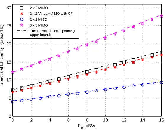
Firstly, we verify the validity and accuracy of the SE upper bound given by Proposition 1
for the Virtual-MIMO system and that considering Ψ =I for the Nt×Nr MIMO case in Fig.
2. For virtual-MIMO, we consider G= 10 dB and γ = 0.25, where the value of G is selected
because of the assumption of short-range cooperation channel. The transmit power of the relay is
smaller than that of the transmitter which justifies the chosen value forγ. We consider bandwidth
Scenario I for the virtual-MIMO using CF protocol. This figure shows that the virtual-MIMO
with CF under Scenario I has a SE performance very close to the MIMO system. We can also
see that the upper bounds are quite tight for the entire range of Pst, regardless of the number of
antennas, no matter for MIMO or Virtual-MIMO. The tightness of the SE upper bounds is very
important to guarantee the accuracy of EE upper bounds.
Using the above settings ofGand γ, we analyze EE of the virtual-MIMO system with CF for
Scenario I and demonstrate the accuracy of the EE upper bound given by Proposition 2 in Fig.
3. As we consider transmit power constraints, the range of SE is limited as shown in this figure,
where the edge of SE for virtual-MIMO is given by (14) and that for MIMO and MISO are given
by (20) and (21), respectively. Fig. 3 (a) shows that the EE upper bounds are very tight to the
Fig. 3 (b) shows how the EE of virtual-MIMO compare to those of the MIMO and MISO
systems by using EE ratios. In the low SE regime, both the ratios EMIMO/ECF and EMISO/ECF
starts from a value slightly larger than 1, which corresponds to the results obtained from (22)
and (23). With SE increasing, virtual-MIMO demonstrates a much better EE performance than
the non-cooperative MISO system, and performs close to the ideal MIMO case in terms of EE.
Virtual-MIMO is thus particularly valuable to realistic wireless communications: With help from
the relay, Virtual-MIMO enables base stations to become more energy efficient, and allows user
devices to reap longer battery life.
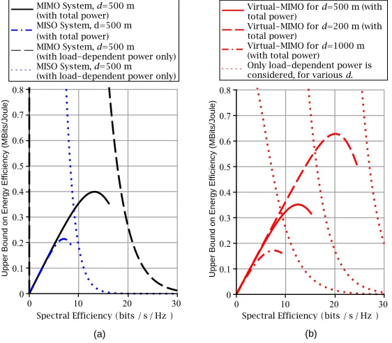
Using the EE upper bounds given by Proposition 2, Fig. 4 shows how load-independent circuit
power and load-dependent power components have meaningful impacts on the overall EE for
both MISO/MIMO and virtual-MIMO with CF. The settings of G and γ remain the same as
above. Fig. 4 (a) shows a trade-off relationship between EE and SE when only load-dependent
power (i.e. NtξsPst) is considered. The EE performance with total power is a combination of the
effects from both load-independent circuit power (i.e.NtPsc) and load-dependent power. That is,
when SE is low, EE is dominated byNtPsc. With SE increasing, the transmit power contributes
more to Ptot; thus, EE increases up to a certain level but finally decreases. A similar trend can
be seen in Fig. 4 (b) for virtual-MIMO, but the load-dependent power is (Ntξs+γ)Pst and the
circuit power is (NtPsc+Prc). Fig. 4 (b) also shows the impact of varying the distance from the
transmitter to the receiver group on EE. A shorter distance (i.e. a smaller value of d) guarantees
a higher EE and vice versa.
Our next analysis demonstrates the impact of different power allocation choices, defined by
different values of γ, on EE of virtual-MIMO with CF for Scenario I. We choose specific
capacity-achieving transmission rates, e.g., SCF= 10,12 bits/s/Hz, and consider G= 10,20 dB.
The results from this scenario are shown in Fig. 5. It is shown that different values ofγ result in
different levels of EE. The upper bound is very tight to the simulated EE, regardless the values
of γ, and can therefore be used to predict the practical EE. Thus it is appropriate to implement
the optimal γ∗ which is computed from (26) to maximize the overall EE. As illustrated in this
equals 0.53 for both SCF= 10 and 12 bits/s/Hz.
B. EE Optimizations
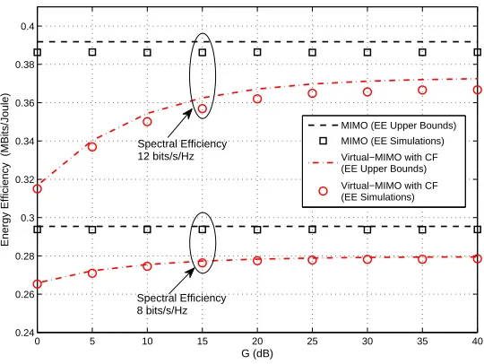
We now demonstrate the optimal EE performance of virtual-MIMO with CF in this subsection,
where optimal power allocation is performed for Scenario I and optimal joint power and
band-width allocation is performed for Scenario II. Specifically, under Scenario I, with the optimal
choices of γ∗ computed from (26), the EE comparisons between virtual-MIMO and MIMO (for
specificSCF = 8,12bits/s/Hz) against the cooperation channel power gainGare shown in Fig. 6.
As the results show, when G is small, EE of virtual-MIMO is impaired by energy consumption
at the relay and also unstable transmission over the weak cooperation channel. As G increases,
the helping relay enables virtual-MIMO to achieve a better EE performance very close to that
of the ideal MIMO case. In addition, with a smaller value of SCF, the EE performance is less
affected by the conditions of the cooperation channel, as the load-independent circuit power is
a dominant factor here.
We now extend the EE performance analysis to Scenario II, where bandwidth allocation needs
to be optimized jointly with power allocation to maximize EE. G= 20 dB is considered in Fig.
7. We can see that the EE performance of virtual-MIMO with CF is much better than that of
the MISO case, even though their performance gap is much smaller compared to Scenario I. In
addition, to illustrate the benefit of CF cooperation for virtual-MIMO, we also show the results
using AF in Fig. 7. As discussed in Section II-C, AF is a special case of CF where half of the
total network bandwidth is allocated for cooperation. As the results demonstrate, CF with equal
bandwidth allocation (i.e., the AF case) is even less energy efficient than MISO; but using the
optimal power and bandwidth allocation, virtual-MIMO with CF outperforms MISO in terms of
EE under most SE values.
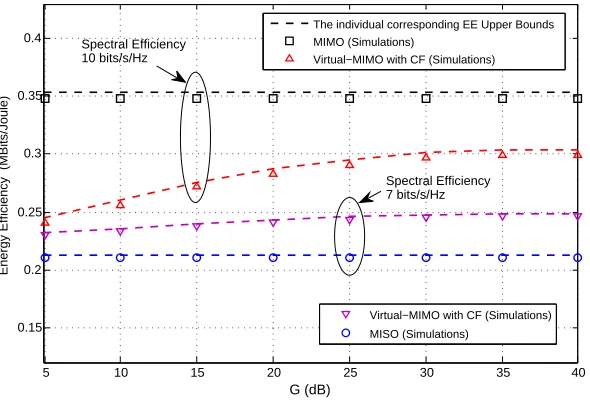
In Fig. 8, EE comparisons among virtual-MIMO, ideal MIMO, and MISO as a function of
G, are presented for different values of SE under Scenario II. Compared to the performance
for Scenario I, a bigger loss exists for virtual-MIMO with CF against MIMO due to the extra
values of G on the EE performance are shown: When SE is low, EE of virtual-MIMO with
CF is less affected by the conditions of the cooperation channel; When SE is high, a larger
value of G guarantees a better cooperation channel and thus results in higher EE performance
of virtual-MIMO.
VI. CONCLUSION
This paper investigates EE performance of a virtual-MIMO system using receiver-side CF
cooperation, where a realistic power model is considered. To account for the cost of cooperation,
the allocation of power as well as bandwidth in the system are studied. We derive a tight
closed-form upper bound for the ergodic capacity of the system, and based on which we propose a
novel and accurate upper bound for EE as a function of SE. The EE upper bound is obtained in
a closed-form expression when an out-of-band channel is used for cooperation. The EE upper
bound exhibits a good accuracy for a wide range of SE values, and thus is utilized for explicitly
tracking the EE performance of MIMO and analytically assessing the EE ratios of
virtual-MIMO over the virtual-MIMO or MISO system.
Based on EE upper bound, we have formulated the EE optimization problem and demonstrated
that for the virtual-MIMO system there exist two ways to improve EE: power allocation between
the transmitter and the relay, and bandwidth allocation between the data and cooperation channels.
Given a target SE, the system EE is maximized by using optimal power and bandwidth allocation,
which provides much insight for designing practical virtual-MIMO systems. Results indicate
that EE performance of virtual-MIMO is sensitive to many factors including resource allocation
schemes and channel characteristics. In addition, EE performance of virtual-MIMO is close to
MIMO when the out-of-band cooperation channel is considered. For the shared-band cooperation
channel, virtual-MIMO with equal bandwidth allocation is less energy efficient than MISO; but
with optimal power and bandwidth allocation, virtual-MIMO outperforms MISO in terms of
EE under most values of SE. Virtual-MIMO is thus particularly valuable to realistic wireless
communications: With the proposed scheme, Virtual-MIMO enables base stations to become
This paper focuses on the 2×2 virtual-MIMO system, i.e. two-antenna transmitter sending
information to two single-antenna receivers. For the virtual-MIMO configuration with more
transmit antennas and more cooperating terminals, EE improvements over MISO can be expected
only when the capacity improvement (because of cooperation) can compensate for the extra
power required at the relays. Extending the analysis to more cooperating terminals, and studying
suitable resource allocation schemes among the relays to guarantee EE benefits are left as future
work.
APPENDIXA
PROOF OFLEMMA1
If Y ∼ CWNr(Nt,Ψ), the density function of Y is given by [25]
pY(Y) =
1 ΓNr(Nt)
[det(Ψ)]−Nt[det(Y)]Nt−Nretr(−Ψ−1Y), Y >0 (29)
where ΓNr(Nt) =π
Nr(Nr−1)/2QNr−1
j=0 Γ(Nt−j) is the multivariate gamma function and Γ(·) is
the gamma function. From the density of Y, we have
E[det(Y)] = 1 ΓNr(Nt)
[det(Ψ)]−Nt
Z
Y>0
[det(Y)]Nt−Nr+1etr(−Ψ−1Y)dY. (30)
Make the change of variate Y =Ψ1/2ZΨ1/2. With Jacobian (dY) = [det(Ψ)]Nr(dZ), we have
E[det(Y)] = 1 ΓNr(Nt)
[det(Ψ)]−Nt
Z
Z>0
[det(Z)]Nt−Nr+1[det(Ψ)]Nt+1etr(−Z)dZ
= 1
ΓNr(Nt)
[det(Ψ)]−Nt[det(Ψ)]Nt+1Γ
Nr(Nt+ 1) = det(Ψ)
NYr−1
j=0
(Nt−j). (31)
This completes the proof.
APPENDIX B
PROOF OF PROPOSITION1
Applying Jensen’s inequality to (9) and when SNR is not low, we have
CCF≤Wlog2E
det
I+ Pst
N0W
Ξ
≈Wlog2E
det
Pst
N0W
Ξ
If He ∼ CNNr,Nt(0,Ψ⊗I), then Ξ ∼ CWNr(Nt,Ψ) where Nt ≥ Nr. Using (8), and denoting
the ergodic capacity upper bound as CbCF, we thus obtain Proposition 1.
APPENDIX C
PROOF OF PROPOSITION2
According to (11), obtaining the expression of EbCF boils down to finding an inverse function
of CbCF in (13), i.e. finding a solution for f−1(CbCF). As CbCF is derived when SNR is not low
according to Proposition 1, we consider the case (GγPst + 2Pst) KtdζN0W in (13). This
assumption is reasonable because that when Pst is small, the value of ECF is dominated by the
circuit powerPsc andPrc as shown in (11). In contrast,ECF is more sensitive and needs a more
accurate expression when Pst is large. Thus when SNR is not low, we have
b
CCF≈W
2 log2
Pst
KtdζN0W
+ 1 + log2
Gγ Gγ+ 2
. (33)
Solving the equation, we obtain
Pst =f−1(CbCF) = 2
SCF
2 − 1
2KtdζN0W
s
Gγ+ 2
Gγ . (34)
Substituting (34) into (11), and let SCF = CWCF we thus obtain (14). Note that the condition of
SCF in (14) is due to the power constraint of 0< Pst ≤Pmax,s.
APPENDIXD
PROOF OFCONVEXITY FOREbCF(γ)UNDERSCENARIOI
Note that proveEbCF(γ) is concave is equivalent to provePtot(γ) is convex. According to (14),
we have
∂Ptot(γ)
∂γ =
∂ ∂γ
"
(2ξs+γξr)2
SCF
2 − 1 2K
tdζN0W
s
Gγ+ 2
Gγ + 2Psc+Prc #
= 2SCF2 − 1
2KtdζN0W(ξrγ
2G+ξ
rγ −2ξs)
q
Gγ+2 Gγ Gγ2
where ∂γ∂ (·) denotes the derivative of a function with respect to the variable γ. Then we have
the second-order derivative of Ptot(γ) with respect to γ
∂2P
tot(γ)
∂γ2 =
∂ ∂γ
∂Ptot(γ)
∂γ
= 2SCF2 − 1
2KtdζN0W(6ξs−ξrγ+ 4ξsGγ)
(Gγ+ 2)Gγ3
q
Gγ+2 Gγ
. (36)
If ξr ≤ 4ξsG, we have ∂2P
tot(γ)
∂γ2 ≥ 0 on γ ∈ (0, Pmax,r/Pst]. Since the scaling factors ξs and ξr
are always natural numbers and in the same order of magnitude as indicated in [8], and as we
are interested in high values of G, it is highly reasonable to assume ξr ≤4ξsG. Thus we have ∂2P
tot(γ)
∂γ2 ≥ 0 and Ptot(γ) is convex on γ ∈(0, Pmax,r/Pst]. This completes the proof that EbCF(γ)
is a concave function on γ ∈(0, Pmax,r/Pst].
APPENDIXE
PROOF OF CONVEXITY FOREbCF(γ, φ)UNDER SCENARIOII
The EE upper boundEbCFfor Scenario II is given by (18), where the function(1+GγP /φ) φ−
1
is strictly increasing on γ ∈(0,1] and φ∈(0,1]and can be fitted by polynomial functions. We
use a quadratic polynomial GγP φ2 to fit (1+GγP /φ)φ−1, so that the total power for the entire
system can be manipulated as
Ptot(γ, φ) = 2Psc+Prc+
(2ξs+γξ√r)KtdζN0W
2Gγφ · q
Gγ(2SCF(1+φ)Gγφ2+ 21+SCF+SCFφ). (37)
The polynomial fitting preserves the original function’s increasing property and helps provide a
closed-form solution forPtot. Proving the convexity ofEbCF(γ, φ)thus boils down to proving the
convexity of Ptot(γ, φ). Based on (37), we have
∂2P
tot(γ, φ)
∂γ2 =
2−1/2+SCF+φSCFK
tdζN0W (−ξrγ+ 4Gγφ2ξs+ 6ξs)
γ2(Gγφ2+ 2)φpGγ2SCF(1+φ)(Gγφ2+ 2) . (38)
Since the scaling factorsξsandξrare always natural numbers and in the same order of magnitude
as indicated in [8] and we are interested in high values of G, it is highly reasonable to assume
ξr ≤ 6ξsPst/Pmax,r+ 4ξsGφ2. Thus we have ∂ 2P
tot(γ,φ)
from (37) we obtain
∂2Ptot(γ, φ)
∂φ2 =
(2ξs+ξrγ)KtdζN0W21/2+SCF+SCFφ
8φ3pGr2SCF(1+φ)(Gγφ2+ 2) ·
G2γ2φ6SCF2 ln2(2) + 4Gγφ4SCF2 ln2(2)
−8Gγφ3SCFln(2) + 4φ2SCF2ln2(2) + 24Gγφ2−16SCFφln(2) + 32
. (39)
As high values of G and SCF are more interested, we have ∂2P
tot(γ,φ)
∂φ2 ≥0 on φ ∈(0,1] as well.
Therefore, on the set of γ ∈ (0, Pmax,r/Pst] and φ ∈ (0,1], the Hessian matrix of Ptot(γ, φ) is
positive semidefinite [23], and thusPtot(γ, φ)is a convex function. This completes the proof that
b
ECF(γ, φ) is concave onγ ∈(0, Pmax,r/Pst] and φ ∈(0,1].
ACKNOWLEDGMENT
This work has been done within a joint project, supported by Huawei Tech. Co., Ltd, China.
REFERENCES
[1] R. Dabora and S. D. Servetto, “Broadcast channels with cooperating decoders,” IEEE Trans. Inform. Theory, vol. 52,
no. 12, pp. 5438–5454, Dec. 2006.
[2] C. T. K. Ng, N. Jindal, A. J. Goldsmith, and U. Mitra, “Capacity gain from two-transmitter and two-receiver cooperation,”
IEEE Trans. Inform. Theory, vol. 53, no. 10, pp. 3822–3827, Oct. 2007.
[3] Z. Ding, K. Leung, D. Goeckel, and D. Towsley, “Cooperative transmission protocols for wireless broadcast channels,”
IEEE Trans. on Wireless Commun., vol. 9, no. 12, pp. 3701–3713, Dec. 2010.
[4] J. Jiang, J. S. Thompson, and H. Sun, “A singular-value-based adaptive modulation and cooperation scheme for
virtual-MIMO systems,”IEEE Trans. Vehicular Technology, vol. 60, no. 6, pp. 2495–2504, July 2011.
[5] J. Jiang, J. Thompson, H. Sun, and P. Grant, “Performance assessment of virtual multiple-input multiple-output systems
with compress-and-forward cooperation,”IET Communications, vol. 6, no. 11, pp. 1456–1465, 2012.
[6] F. Heliot, M. Imran, and R. Tafazolli, “On the energy efficiency-spectral efficiency trade-off over the MIMO Rayleigh
fading channel,”IEEE Trans. Communications, vol. 60, no. 5, pp. 1345–1356, May 2012.
[7] Y. Chen, S. Zhang, S. Xu, and G. Li, “Fundamental trade-offs on green wireless networks,”IEEE Commun. Mag., vol. 49,
no. 6, pp. 30–37, June 2011.
[8] G. Auer, V. Giannini, C. Desset, I. Godor, P. Skillermark, M. Olsson, M. Imran, D. Sabella, M. Gonzalez, O. Blume, and
A. Fehske, “How much energy is needed to run a wireless network?”IEEE Wireless Communications, vol. 18, no. 5, pp.
40–49, Oct. 2011.
[9] Y. Chen, S. Zhang, and S. Xu, “Characterizing energy efficiency and deployment efficiency relations for green architecture
[10] Y. Yao, X. Cai, and G. Giannakis, “On energy efficiency and optimum resource allocation of relay transmissions in the
low-power regime,”IEEE Trans. Wireless Commun., vol. 4, no. 6, pp. 2917–2927, Nov. 2005.
[11] X. Cai, Y. Yao, and G. B. Giannakis, “Achievable rates in low-power relay links over fading channels,” IEEE Trans.
Commun., vol. 53, no. 1, pp. 184–194, 2005.
[12] J. Gomez-Vilardebo, A. Perez-neira, and M. Najar, “Energy efficient communications over the AWGN relay channel,”
IEEE Trans. Wireless Commun., vol. 9, no. 1, pp. 32–37, Jan. 2010.
[13] S. Cui, A. Goldsmith, and A. Bahai, “Energy-efficiency of MIMO and cooperative MIMO techniques in sensor networks,”
IEEE Journal on Selected Areas in Commun., vol. 22, no. 6, pp. 1089 –1098, Aug. 2004.
[14] S. Jayaweera, “Virtual MIMO-based cooperative communication for energy-constrained wireless sensor networks,”IEEE
Trans. Wireless Commun., vol. 5, no. 5, pp. 984–989, May 2006.
[15] Y. Qi, R. Hoshyar, M. Imran, and R. Tafazolli, “H2-ARQ-relaying: Spectrum and energy efficiency perspectives,”IEEE
Journal on Selected Areas in Communications, vol. 29, no. 8, pp. 1547–1558, Sep. 2011.
[16] D. Tse and P. Viswanath,Fundamentals of Wireless Communication. New York, NY, USA: Cambridge University Press,
2005.
[17] G. Auer and et al., “D2.3: Energy efficiency analysis of the reference systems, areas of improvement and target breakdown,”
INFSO-ICT-247733 EARTH (Energy Aware Radio and NeTwork TecHnologies), Tech. Rep., Nov. 2010.
[18] Y. Qi, M. A. Imran, D. Sebella, B. Debaillie, R. Fantini, and Y. Fernandez, “Deployment opportunities for increasing
energy efficiency in LTE-advanced with relay nodes,” in29th Meeting of WWRF, 2012, pp. 1–5.
[19] Y. Liang, V. V. Veeravalli, and H. V. Poor, “Resource allocation for wireless fading relay channels: Max-min solution,”
IEEE Trans. Inform. Theory, vol. 53, no. 10, pp. 3432–3453, Oct. 2007.
[20] A. Host-Madsen and J. Zhang, “Capacity bounds and power allocation for wireless relay channels,”IEEE Trans. Inform.
Theory, vol. 51, no. 6, pp. 2020–2040, June 2005.
[21] I. Krikidis, J. Thompson, S. McLaughlin, and N. Goertz, “Optimization issues for cooperative amplify-and-forward systems
over block-fading channels,”IEEE Trans. on Vehicular Technology, vol. 57, no. 5, pp. 2868–2884, Sept. 2008.
[22] T. T. Kim, M. Skoglund, and G. Caire, “Quantifying the loss of compress-forward relaying without Wyner-Ziv coding,”
IEEE Trans. Inform. Theory, vol. 55, no. 4, pp. 1529–1533, April 2009.
[23] S. Boyd and L. Vandenberghe,Convex Optimization. Cambridge University Press, 2004.
[24] L. Zhang, Y. Xin, Y.-C. Liang, and H. Poor, “Cognitive multiple access channels: optimal power allocation for weighted
sum rate maximization,”IEEE Transactions on Communications, vol. 57, no. 9, pp. 2754 –2762, Sep. 2009.
Relay
Short range cooperation channel
Destination
T
ra
n
sm
itt
er
Pst
W,H
Wr, G
Receiver Side Data channel
Pst
[image:27.612.171.435.72.242.2]Prt
Fig. 1. System model of the virtual-MIMO system (Nt=Nr = 2)
TABLE I
OPTIMIZATIONALGORITHM FOR(27)UNDERBANDWIDTHSCENARIOII
Initialize: k = 0, ρ(0), µ(0), γ(0), and φ(0). Repeat
(a) Obtain the possible optimal values γ†(ρ(k), µ(k)) and φ†(ρ(k), µ(k)) by solving
∂ECF(γ, φ)
∂γ φ=φ(k) =ρ
(k) and ∂ECF(γ, φ)
∂φ γ=γ(k) =µ
(k),
where ECF(γ, φ) is giving by (18).
(b) Update the parameters γ(k), φ(k), ρ(k+1), and µ(k+1) by
(
γ(k) =γ†(ρ(k), µ(k)), φ(k)=φ†(ρ(k), µ(k));
ρ(k+1) =
h
ρ(k)−τ1(k)g1(k) i+
, µ(k+1) =
h
µ(k)−τ2(k)g(2k) i+
.
(c) Calculate the Lagrangian function L(γ(k), φ(k), ρ(k), µ(k)). (d) k=k+ 1.
[image:27.612.83.524.418.641.2]TABLE II
SIMULATIONPARAMETERS(VALUES OFPOWERMODELPARAMETERS ARESUGGESTED BY[8]AND[18]).
Parameter Value Parameter Value
N0 -174 dBm/Hz Psc(Macro) 130 W
W 10 MHz ξs(Macro) 4.7
Kt 10−3 Pmax,r(relay) 5 W
d 500 m Prc(relay) 14.3 W
ζ 3.5 ξr(relay) 2.8
Pmax,s(Macro) 20 W
0 2 4 6 8 10 12 14 16
0 5 10 15 20 25 30
Spectrual Efficiency (Bits/s/Hz)
P st (dBW) 2 × 2 MIMO
2 × 2 Virtual−MIMO with CF 2 × 1 MISO
3 × 3 MIMO
[image:28.612.165.444.409.629.2]The individual corresponding upper bounds
Fig. 2. Simulation results and upper bounds of the ergodic capacity for Nt×Nr MIMO and virtual-MIMO systems. (For
0 5 10 15 0
0.05 0.1 0.15 0.2 0.25 0.3 0.35 0.4
Energy Efficiency ( MBits/Joule)
Spectral Efficiency (bits/s/Hz)
(a)
MIMO (Simulations) MIMO (UB) Virtual−MIMO (Simulations) Virtual−MIMO (UB) MISO (Simulations) MISO (UB)
0 10 20 30
0 0.5 1 1.5
Energy Efficiency Ratios
Spectral Efficiency (bits/s/Hz) (b)
EMIMO/ECF EMISO/ECF
Performance trend of EMIMO/ECF Performance trend of EMISO/ECF
Fig. 3. EE performance of virtual-MIMO with CF for bandwidth Scenario I, compared with those of MISO and MIMO systems. (For virtual MIMO,G= 10dB andγ= 0.25are considered.)
(a) (b)
[image:29.612.157.443.93.356.2]Upper Bound on Energy Efficiency (MBits/Joule) Upper Bound on Energy Efficiency (MBits/Joule)
[image:29.612.164.445.416.662.2]γ
[image:30.612.177.436.90.328.2]Upper Bound on Energy Efficiency (MBits/Joule)
Fig. 5. The effects of varying the values of γ on the EE performance of the virtual-MIMO system with CF by setting
SCF= 10,12bits/s/Hz andG= 10,20dB under bandwidth Scenario I.
0 5 10 15 20 25 30 35 40
0.24 0.26 0.28 0.3 0.32 0.34 0.36 0.38 0.4
Energy Efficiency (MBits/Joule)
G (dB)
MIMO (EE Upper Bounds) MIMO (EE Simulations) Virtual−MIMO with CF (EE Upper Bounds) Virtual−MIMO with CF (EE Simulations)
Spectral Efficiency 12 bits/s/Hz
Spectral Efficiency 8 bits/s/Hz
[image:30.612.168.438.431.634.2]0 5 10 15 0 0.05 0.1 0.15 0.2 0.25 0.3 0.35 0.4
Energy Efficiency ( MBits/Joule)
Spectral Efficiency (bits/s/Hz)
(a)
0 5 10 15 20 0 0.2 0.4 0.6 0.8 1 1.2 1.4 1.6 1.8 2
Energy Efficiency Ratios
Spectral Efficiency (bits/s/Hz) (b)
MIMO (Upper Bound) Virtual MIMO with CF (Upper Bound) Virtual MIMO with CF (Simulations) MISO (Upper Bound) Virtual MIMO with AF (Upper Bound) Virtual MIMO with AF (Simulations)
EMISO/ECF
Performance trend of EMISO/ECF EMISO/EAF
[image:31.612.164.445.104.344.2]Performance trend of EMISO/EAF
Fig. 7. EE performance of the virtual-MIMO system under bandwidth Scenario II with setting G= 20dB. (Optimal power allocation is performed for the AF case, while optimal joint power and bandwidth allocation is performed for CF.)
5 10 15 20 25 30 35 40
0.15 0.2 0.25 0.3 0.35 0.4 G (dB)
Energy Efficiency (MBits/Joule)
The individual corresponding EE Upper Bounds MIMO (Simulations)
Virtual−MIMO with CF (Simulations)
Virtual−MIMO with CF (Simulations) MISO (Simulations)
Spectral Efficiency 7 bits/s/Hz Spectral Efficiency
10 bits/s/Hz
[image:31.612.158.453.447.647.2]