Adaptive deformation correction of depth from defocus for object reconstruction

http://wrap.warwick.ac.uk/

Original citation:

Li, Ang, Tjahjadi, Tardi and Staunton, Richard. (2014) Adaptive deformation correction of depth from defocus for object reconstruction. Journal of the Optical Society of America A: Optics, Image Science and Vision, Volume 31 (Number 12). pp. 2694-2702. ISSN 1084-7529

Permanent WRAP url:

http://wrap.warwick.ac.uk/66099

Copyright and reuse:

The Warwick Research Archive Portal (WRAP) makes this work of researchers of the University of Warwick available open access under the following conditions. Copyright © and all moral rights to the version of the paper presented here belong to the individual author(s) and/or other copyright owners. To the extent reasonable and practicable the material made available in WRAP has been checked for eligibility before being made available.

Copies of full items can be used for personal research or study, educational, or not-for-profit purposes without prior permission or charge. Provided that the authors, title and full bibliographic details are credited, a hyperlink and/or URL is given for the original metadata page and the content is not changed in any way.

Publisher statement:

This paper was published in Journal of the Optical Society of America A: Optics, Image Science and Vision and is made available as an electronic reprint with the permission of OSA. The paper can be found at the following URL on the OSA website

http://dx.doi.org/10.1364/JOSAA.31.002694 .

Systematic or multiple reproduction or distribution to multiple locations via electronic or other means is prohibited and is subject to penalties under law.

A note on versions:

The version presented here may differ from the published version or, version of record, if you wish to cite this item you are advised to consult the publisher’s version. Please see the ‘permanent WRAP url’ above for details on accessing the published version and note that access may require a subscription.

Adaptive Deformation Correction of Depth from

Defocus for Object Reconstruction

Ang Li,

Tardi Tjahjadi,

and Richard Staunton

1_{School of Engineering, University of Warwick,}

Coventry, West Midlands, CV4 7AL, UK

Abstract

The accuracy of 3-dimensional object reconstruction using Depth from Defocus (DfD) can be severely reduced

by elliptical lens deformation. This paper presents two correction methods, correction by deformation

cancellation (CDC) and correction by least squares fit (CLSF). CDC works by subtracting the current

deformed depth value by a pre-stored deformed value, and CLSF by mapping the deformed values to the

expected values. Each method is followed by a smoothing algorithm to address the low-texture problem of

DfD. Experiments using four DfD methods on real images show that the proposed methods effectively and

efficiently eliminate the deformation.

OCIS codes: 100.3010, 100.6890

http://dx.doi.org/10.1364/XX.99.099999

1. Introduction

Image blur is the cue for depth measurement in a passive depth from defocus (DfD) method

for 3-dimensional (3D) object reconstruction based on image blurring. In Pentland’s DfD

scheme [1, 2], a pinhole camera setting is used to capture a first image so that every point

of the image is in focus, while a wider-aperture camera setting is used to capture a second

blurred image. The Gaussian point spread function (PSF) is used to model the blur and

is convolved with one focused sub-image to give a blurred sub-image. The standard

devi-ation of the resulting PSF is used to estimate the depth map of the object, and thus the

reconstruction of the 3D object.

It is not necessary for one of the images to be captured with a pinhole camera setting

which generates very large diffraction. In Subbarao’s method [3], the two images are captured

with any different known parameters. The standard deviations of the Gaussian PSF that

correspond to the two images are then determined. In both methods the depth is estimated

using inverse filtering technique, i.e., the parameter of the PSF is firstly determined for two

captured images, and are then used to obtain depth. One major problem in passive DfD is

the shift-variance of PSF and thus different PSFs are used for different pairs of sub-images.

Based on the work in [3], Markov Random Field is used in [4] to model the intensity and

depth value of every image pixel, so that the PSF can be modified by considering the

neigh-bouring pixels. Thus the method enforces smoothness while preserving discontinuities in

depth. Finally, a maximum a posterior function is maximised using simultaneous annealing

to obtain the optimal depth estimation.

The depth map of an object can also be estimated from the convolutional ratio, which is

convolved with the PSF of the first image to give the PSF of the second [5]. A pre-computed

lookup table of convolutional ratios and their corresponding depth value is then searched

to estimate depth. To reduce the edge effect of DfD, the PSF is modelled as a downturn

quadratic, so that a linear procedure can be used to regularise the shape of the PSF to

reduce the edge effect and noises.

The work in [6] argues that the approach in [1] requires low-order regression fit in the

frequency domain of every local region in order to calculate the defocus parameter, which is

not well suited to the optical system. Instead, the entropy concept is applied to image blur

The work in [7] argues that previous approaches assume the depth to be constant over

fairly large local region and consider the blurring to be shift-invariant over those local regions,

which leads to errors when the neighbourhood regions are not considered. Two methods

are proposed to address this problem. The first method models the DfD system as block

shift-variant, where the PSF incorporates the interaction of the blur from the surrounding

regions. The second method is based on the space-frequency representation of the local

regions.

The pattern on an object results in different spatial frequencies that have different depth

response, where the depth of low-frequency pattern changes rapidly with the normalised

image ratio (NIR) and that of high-frequency pattern changes slowly [8]. To achieve

fre-quency independence, Watanabe and Nayer [8] model the image information in the frefre-quency

domain as a third order polynomial of depth and frequency, the coefficients of which are

expressed in rational forms to generate the rational operators. Depth is estimated using the

rational operators. Raj and Staunton [9] proposed a set of operators that estimate depth

more accurately.

In [10], an orthogonal projector that spans the null-space of an image of a specific depth

is used for depth estimation. Images are captured for a number of different depth levels,

and the corresponding orthogonal projectors are generated. During depth computation,

each sub-image is multiplied by every projector, which corresponds to a specific depth. The

depth that corresponds to the projector that gives the smallest product is the estimated

depth.

Other recent approaches to DfD include the following. In [11], an unscented Kalman filter

is used, and the defocus parameter is measured by gradient descent, and the mathematical

model is the traditional convolution between focused image and the PSF. Both motion blur

and optical blur are decoupled by modelling them as convolution with the PSF due to optical

blur and then with the PSF due to motion blur. Methods based on coded apertures are

reported in [12, 13], which optimise the PSF by modifying the aperture shape. These use

complex statistical models and are computationally expensive. The work in [14] improves

DfD by manipulating exposure time and guided filtering. The work in [15] improves object

reconstruction by minimising the information divergence between the estimated and actual

blurred images via geometric optics regularisation.

an entire image, so that the same DfD framework can be used for every pixel or sub-image.

However, this assumption is violated for most off-the-shelf camera lenses [16–18], which

causes the depth map of a flat surface to be approximately a 3D quadratic surface, i.e.,

the depth map is severely deformed by the surface peripheral that is of considerably high

curvature.

A correction method based on two-step least squares fit is incorporated to the state of the

art Li’s DfD method in [19]. First, the depth offset is modelled as a third order polynomial

of the x coordinate, y coordinate and the input (deformed) depth value, i.e.

D_{(x, y) =~c1(1) +}

4 X

i=2

~c1(i)xi−1 + 7 X

i=5

~c1(i)yi−4

+

10 X

i=8

~c1(i)(Ui(x, y))i−7, (1)

where the set of coefficients c1 is found by least squares fit, and Ui is the deformed depth. Second, the corrected depth is modelled as another third order polynomial of the x

coordi-nate, y coordinate and the depth offset value, i.e.,

U_{o(x, y) =~c2(1) +}

4 X

i=2

~c2(i)xi−1+ 7 X

i=5

~c2(i)yi−4

+

10 X

i=8

~c2(i)(D(x, y))i−7, (2)

where the set of coefficients~c2 is found by another least squares fit. The corrected depth is

finally computed using Eqn. (2).

This method cannot work well with other DfD methods because: (a) it is based on

two-step least squares fit, and the errors generated from the first fit in Eqn. (1) propagates to

the second fit in Eqn. (2), which generates additional errors; (b) it uses global fit rather than

local fit, generating only one set of coefficients for all locations of the depth maps, which

may not be always valid for all locations; and (c) it cannot avoid spurious depth results at

low-texture regions since it does not involve any analysis on the frequency content of input

images.

In this paper, we propose two correction methods: correction by deformation cancellation

(CDC) and correction by least squares fit (CLSF). The first method works by obtaining a

number of correction patterns that are used to cancel out the deformation. The second works

fit. The other main contribution is that the methods also address the deformation problem

which is spatially variant in terms of 3 dimensions: horizontal and vertical dimensions of

the depth map and the depth of each pixel. Experiments are performed with four different

DfD methods to demonstrate that the correction methods can potentially be adapted to all

other DfD approaches.

This paper is organised as follows. Section 2 introduces the deformation problem.

Sec-tion 3 and SecSec-tion 4 present CDC and CLSF, respectively. SecSec-tion 5 proposes a

post-processing algorithm which addresses the low-texture problem of the input images. Section 6

presents both quantitative and qualitative evaluation of the two correction methods. Finally

Section 7 concludes the paper.

2. The depth-variant elliptical deformation problem

Since most of the off-the-shelf camera systems consist of spherical lenses with flat sensors,

they naturally form a focused image on a curved surface rather than the flat sensor surface

[16–18]. This adverse effect is mainly due to two types of optical aberration, astigmatism

and field curvature. Astigmatism causes the tangential component of a fan of rays to be

focused at different surface than the sagittal component, both of which are curved. Field

curvature is similar, where the tangential and sagittal components are the same. Both

aberrations are off-axis, with no effect along the optical axis and greater effect at locations

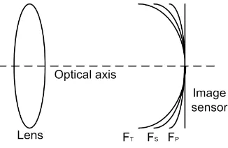
further way from the optical axis. Fig. 1 illustrates these two aberrations, whereFT and FS

respectively represent the actual focusing surface of the tangential and sagittal components

of astigmatism, and FP represents that of field curvature.

Fig. 1. Deformation due to astigmatism (FT andFS) and field curvature (FP).

being defocused differently at different (x, y) locations. The resulting depth map is thus a

deformed surface. Moreover, the addition of defocusing due to these two aberrations to the

defocusing due to depth makes the deformation depth-dependent, considering depth is not

a simple linear combination of defocus amount.

Furthermore, a number of other problems may occur during manual DfD input image

acquisition, where the lens is fixed and the image sensor plane is moved along the optical

axis. These include: (a) the sensor cannot be aligned perfectly parallel to the lens; (b)

the angle between sensor and lens changes during movement; and (c) the image centre is

not aligned with the optical axis. They in turn result in orientation change of the curved

focusing surface, and the peak of the surface not being aligned with the image centre.

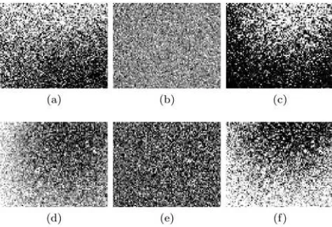
Fig. 2 illustrates the deformation problem using Subbarao’s method [3]. The working

range is set to be within [887,933] mm away from the lens. The grey levels of the

grey-coded depth map of a flat surface without any deformation should be uniformly distributed.

The depth map of a flat surface which is 933 mm away from the lens (i.e., furthest away)

shown in Fig. 2(a) has very strong elliptical deformation with its centre at the bottom right

corner. The centre does not intercept with the optical axis (i.e., not at the centre of the

depth map) due to an inevitable misalignment during the manual sensor-lens decoupling

required to obtain the input images. The deformation may be eliminated by subtracting the

depth map with the depth map of a flat surface at the specific depth (i.e., the correction

pattern), then adding the distance corresponding to that pattern (the offset), thus flattening

the general shape while correcting the depth.

Note that in Fig. 2(a)-(c) the depth maps are plotted with the same scale, where the

darkest and the brightest represent the depth of 925 mm and 940 mm, respectively. Fig.

2(d)-(f) are also plotted with the same scale, where the darkest and the brightest represent 880

mm and 900 mm, respectively.

Fig. 2(b) shows that the surface in (a) is effectively corrected by the pattern at the

furthest point, as seen by the relatively uniform distribution of the grey levels. It is assumed

that the correction patterns within the working range have the same shape. Fig. 2(c) shows

that this assumption is invalid when the surface in (a) is corrected by the correction pattern

at the nearest point, which exacerbates the deformation.

Similar results are shown in Fig. 2(d-e) where the depth map at the nearest point is

Fig. 2. Grey-coded depth maps illustrating the deformation problem and the depth dependence

problem with Subbarao’s method [3]: (a) the furthest flat surface with deformation; (b) surface

(a) corrected using the furthest correction pattern; (c) surface (a) corrected using the nearest

correction pattern; (d) the nearest flat surface with deformation; (e) surface (d) corrected using

the nearest pattern; and (f) surface (d) corrected using the furthest pattern.

respectively. Similar depth maps are also obtained using Favaro’s method [10] and Raj’s

method [9], i.e., the deformation problem is depth dependent and the above correction

method is inadequate.

Since the cause of such a deformation involves the two types of optical aberrations and

errors in input image acquisition, complex optical measurements and mathematical

mod-elling are required for deformation removal methods via correction of input images. We take

a different approach by treating the entire DfD system as a black box, and finding the

rela-tionship between sampled input depth maps and the corresponding output depth maps. Our

methods including CDC and CLSF prove effective, not involving complex measurements,

and can potentially be applied to any DfD methods.

3. Correction by deformation cancellation

One means of removing the depth-variant deformation of a DfD method is to cancel the

deformation with the stored deformation. We refer this method as CDC. Each correction

pattern is a depth map acquired by the DfD method, with a flat surface placed at different

equal incrementing distance to the camera until the closest working limit. The patterns are

numbered as 1,2,3 ... M from the furthest limit to the closest limit, where M is the total

number of patterns. We refer these numbers as correction pattern indices (CPI), and their

corresponding depth as the depth offset. The depth value of every location of each pattern

is called correction pattern value (CPV).

Correction is achieved by subtracting the deformed depth value at every location in the

depth map, i.e., U_{i, by the corresponding CPV of a correction pattern} U_{c with the most}

suitable CPI,vopt, plus the actual depth of the flat surface used to the obtain the correction

pattern with index vopt (i.e., w~(vopt), or the depth offset, i.e.,

U_{o(x, y) =}U_{i(x, y)−}U_{c(x, y, vopt) +w~(vopt), (3)}

where (x, y) is the spatial index of the current pixel being corrected, and U_{o is the output}

corrected depth. The CPI v which corresponds to depth nearest to the deformed depth is

given by

vopt = argmin v∈[1,M]

|U_{i(x, y)−}U_{c(x, y, v)|. (4)}

Note also that U_{c(x, y, vopt) is the depth value at a given location with similar deformation}

to U_{i(x, y). w~(vopt) is the depth of a flat surface used to obtain} U_{c for all locations, and it}

is only used to shift U_{i(x, y)−}U_{c(x, y, vopt) to its expected value.}

Using Eqn. (4) to search for the nearest CPI may give inaccurate results since the single

deformed depth may be an unreliable input to Eqn. (3). To reduce inaccuracy, the optimal

CPI is found within a local region R _{of size (2N + 1)×(2N + 1) centred at the current}

location (x, y), i.e.,

vopt = argmin v∈[1,M]

N

X

i=−N N

X

j=−N

|U_{i(x, y)−}U_{c(x−i, y−j, v)|. (5)}

In practical applications, N = 1 is a good choice. Eqn. (5) may not always produce the

minimum residual (i.e., its argument of argmin) that is close to zero, i.e., no pixels in the

local region are quite similar to the current input pixel. Thus, this problem is addressed by

interpolation using the two nearby residuals.

The interpolation process is illustrated in Fig. 3(a) for the case where the residual of

the left neighbouring CPI is smaller than the right neighbouring CPI, and similarly for the

found. In this example, the minimal residual of 2.1 is found at CPI being 4. The two

adjacent CPIs are 3 and 5, and their residuals are 3.2 and 5.7, respectively.

Fig. 3. (a) Interpolation to find the improved CPI. Key: stem plot with asterisks - the smallest

residual value and its two nearest values; dashed lines - the interpolated curve; circle - the minimal

of the curve. (b) The second step of interpolation. Key: stem plots with asterisks - the CPV

where the estimated index falls in between; dashed line - the straight line connecting both CPV’s

coordinates; circle - the estimated CPV.

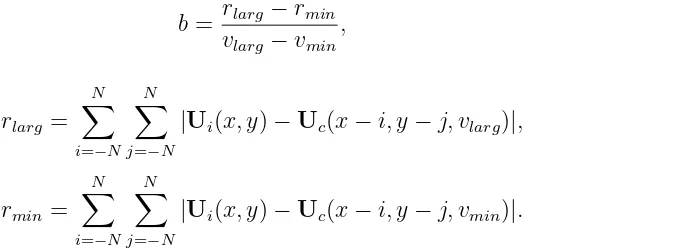
Second, the gradient of the line passing through the minimal CPIvmin and the CPI with

larger residual vlarg is given by

b = rlarg−rmin

vlarg−vmin

, (6)

where

rlarg = N

X

i=−N N

X

j=−N

|U_{i(x, y)−}U_{c(x−i, y−j, vlarg)|, (7)}

rmin = N

X

i=−N N

X

j=−N

|U_{i(x, y)−}U_{c(x−i, y−j, vmin)|. (8)}

In this example, it is the gradient of the line passing CPI=4 and CPI=5 on the right in

Fig. 3(a). This gives the equation of the line

y =bx+rmin−bvmin. (9)

Third, a line with the negative gradient that passes through the other adjacent CPIvsmall

is plotted, the equation of which is

y=−bx+rsmall+bvsmall, (10)

where

rsmall = N

X

i=−N N

X

j=−N

In this example, it is the line on the left in Fig. 3(a). Fourth, the interpolated CPI is the

horizontal coordinates of the intersection of the two lines with Eqn. (9) and (10).

In cases where the minimal CPI does not have left or right adjacent values, the estimated

CPI is the minimal CPI itself. The interpolation method is based on an assumption that

(vmin, rmin), (vsmall, rsmall) and (vlarg, rlarg) are three samples of a conditional first order

polynomial curve (or a curve consisting of two straight lines). In addition, its average shape

is assumed to be symmetrical to v = vopt which produces minimal estimation error. Thus,

the gradient of the left line is the negative of the right line.

Finally, since the interpolated CPI is in-between the CPI with smallest residual (4 in this

case) and the one with second smallest residual (3 in this case), and the CPVs of them are

known (810 for CPI=3 and 816 for CPI=4 as shown in Fig. 3(b)), the final estimate of the

CPV can be found by a simple linear interpolation as illustrated in the figure.

4. Correction by least squares fit

In [19], we presented a correction method based on least squares fit as part of Li’s DfD

method. First, the CPI is found by least squares fit and CPV is then found by another

least squares fit. Not only are the two fitting procedures unnecessary, accumulative errors

are generated that deform the resulting depth map. In this paper, we propose another

correction by least squares fit, CLSF, which finds the mapping from the deformed depth to

the corrected depth directly with least squares fit.

The corrected depth is modelled as a third order polynomial of the spatial indices and

the deformed depth U_{i, i.e., the corrected depth}

U_{o(x, y) =~c3(1) +}

4 X

i=2

~c3(i)xi−1+ 7 X

i=5

~c3(i)yi−4

+

10 X

i=8

~c3(i)(Ui(x, y))i−7 , (12)

where~c3is the set of coefficients of the fitted polynomial when sufficient samples are collected

forU_{o and}U_{i. In contrast with the correction method in [19], CLSF only requires one least}

squares fit, and thus avoids any accumulative error. However, the output depth may not

be a perfect third order polynomial of the spatial indices. To address this problem, the

coefficients are used. The number of regions is set to 9 in our experiments.

Note that the purpose of CLSF is not to reproduce the deformed depth map using (x, y)

coordinates. Rather, it is to find the corrected depth with three input variables: x

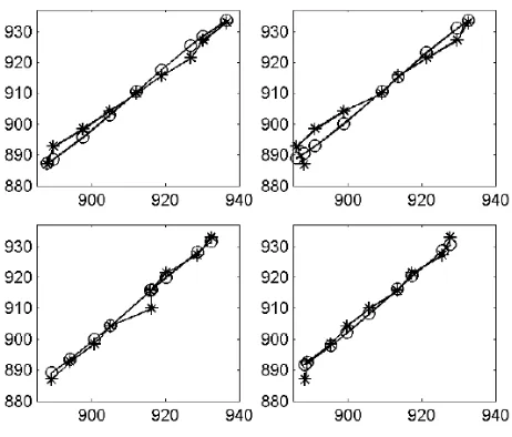
co-ordinate, y coordinate and the input uncorrected depth value at (x, y). Fig. 4

demon-strates that third order polynomial is an appropriate model with Subbarao’s method [3].

Since it is impossible to show all locations, only four samples from all (x, y) locations

are shown. These four samples are at (1/3 width,1/3 height), (1/3 width,2/3 height),

(2/3 width,1/3 height), and (2/3 width,2/3 height). Each sample plot consists of 9 sample

values of depth. Fig. 4 shows that the third order polynomial reproduces/learns the mapping

from uncorrected to corrected depth value reasonably well, capturing the general trend of

the original mapping curves with only a small amount of errors.

Fig. 4. Fitting corrected depth with third order polynomial illustrated with Subbarao’s method

[3] using four (x, y) samples. Horizontal axis: uncorrected depth in mm. Vertical axis: corrected

or expected depth in mm. Key: ◦- corrected depth; ∗ - expected depth.

5. Post-processing for low-texture region

When the target object surface has little texture, there is insufficient information to retrieve

depth. Thus, spurious results are produced such as an extremely low or an extremely high

depth value. We assume the low-texture region to have high correlation with its rich-texture

is produced to identify low-texture regions in the input depth map D_{; (2) Every individual}

region is identified and set to no-value; and (3) Each region is filled with 2-dimensional (2D)

least squares fit.

In the first step, the NIR map [8] used to calculate depth map is computed by

R₌ I1 −I2

I₁₊I₂, (13)

where I_{1 and} I_{2 are the far-focused and near-focused images respectively. Let} R_{loc denote}

every local region of R_{, a confidence map is then produced by evaluating the variance of}

R_{loc, i.e.,}

g = 1

Ng Ng

X

k=1

(~r(k)−µ)2, (14)

where Ng is its total number of elements, µ is the mean of ~r, and ~r is the 1-dimensional

vector created by concatenating every row of R_{loc, i.e.,}

~r(Ncol ·(i−1) +j) =Rloc(i, j), (15)

and Ncol is the number of columns in Rloc.

The variance g is computed for every local region to form the confidence map G_{. In this}

way, low-texture regions corresponding to low variances are readily identified.

In the second step, a mask matrix B _{is initialised as a zero matrix of the same size asG}

by

B_{(x, y) =}   

 

1,if G_{(x, y)> T}

0,otherwise,

(16)

where T is the variance threshold which is set typically to 0.0144. Since the NIR ranges

from 0 to 1, we empirically define the low-texture region to have standard deviation of less

than 0.12, which corresponds to a variance of 0.0144. B _{indicates the locations of the}

low-texture pixels. Pixels of the corresponding locations of the input depth map P_{are set to be}

no-value, which are re-estimated later.

There may be several unconnected low-texture regions that need to be addressed

sepa-rately. With B _{as its input, Moore-Neighbour tracing [20] is used to find all unconnected}

low-texture regions defined by their boundary pixels’ coordinates.

In the third step, 2D linear regression is used to model the depth values of each region as a

i.e.,

ˆ

P_{(x, y) =~c4(1) +}

4 X

i=2

~c4(i)xi−1 + 7 X

i=5

~c4(i)yi−4

+

10 X

i=8

~c4(i)(P(x, y))i−7,∀ P(x, y)6= no-value, (17)

where ˆP _{is the a rectangular region of} B _{which completely covers the low-texture region,}

and~c4 is the set of coefficients obtained by least squares fit.

Fig. 5 illustrates the identification of ˆP_{. In this example,}B_{is a 7×7 binary image, where}

the white pixels correspond to the low-texture region, as shown in the left plot. There is only

one such region for simplicity in illustration. Moore-Neighbour tracing algorithm uses this

image as input and returns the indices of all the boundary pixels, which are drawn in grey

in the middle plot. ˆP _{is then selected as the rectangle that fully covers this region leaving}

one-pixel margin around its boundaries, as shown in the non-black region in the right plot.

We leave this margin because if the region was rectangular, there would be no sampling data

for the least squares fit. After~c4 is estimated, Eqn. (17) is used to re-estimate the depth of

the no-value pixels. This process is repeated for all remaining low-texture regions.

Fig. 5. An example of using Moore-Neighbour algorithm to find input samples for least squares

fit: left: input binary image with a single low-texture region denoted in white; middle: boundary

pixels in grey are identified; right: grey region is identified as the input samples.

6. Experiments

6.A. Experiments condition

The experimental settings used in this paper are identical to those in [19] and as follows. A

50 mm professional lens with a telecentric aperture [21] of 12.8 mm was used for the DfD

maximum radius of the blur circle is 2.703 pixels, which is equivalent to 2.703×7.4−3 _{= 0.0200}

mm.

The working range is set to be [887,933] mm away from the lens. A PC with an Intel Core

i7 @ 3.40 GHz processor was used for data processing. Four Matlab programs were written

for the four DfD methods to evaluate the correction algorithm. The first is the classical

generic Subbarao method [3], the second is learning based Favaro’s method [10], the third

is the RO based Raj’s method [9], and the fourth is the Li’s method [19].

Fig. 6. Quantitative evaluation of the correction method using Subbarao’s method [3] (column 1),

Favaro’s method [10] (column 2), Raj’s method [9] (column 3) and Li’s method [19] (column 4).

Key: ⋄- expected depth;∗ - uncorrected result;◦- corrected with CDC;▽- corrected with CLSF.

Row 1: estimated depth (vertical axis) against expected depth in mm (horizontal axis). Row 2:

RMSE in mm against depth. Row 3: variance in mm2 against depth.

Input grey-level images with a resolution of 640 x 480 pixels are used. Each image pair

for DfD is divided into a number of contiguous 7×7 sub-image pairs where each iteration

of DfD estimation is performed. Thus the resolution of the depth map is 68×91 pixels. A

mm away from the camera, with an increment of 2 mm. Thus, 24 pairs of DfD input images

were captured and 24 correction patterns were generated, while the corresponding offsets

are from 933 mm to 887 mm incremented by 2 mm.

6.B. Quantitative experiments

The correction methods, CDC and CLSF, are applied to the four DfD methods mentioned in

Section 6.A. Fig. 6 shows the results where 9 deformed depth maps are used as the inputs,

which were obtained with a flat surface moved from 933 mm to 887 mm away from the

camera. The plots in the first row are obtained by averaging the value of each depth map;

those in the second row are obtained by calculating the root mean square error (RMSE)

between the estimated and expected depth for each pixel and taking the average over each

depth map; those in the third row are generated by evaluating the variance of each depth

map. Thus, the first row shows the average accuracy, the second row indicates the accuracy

over the depth map and the third row shows the noise performance.

Note that the experiments are to evaluate the performance of the two correction methods,

i.e., not to compare the four DfD methods where the basic difference is whether a PSF model

is used or the PSFs used. PSF parameter calibration is involved in [3] and [19], while no

calibration is required for the others. Thus, these methods produce the better accuracy.

This is verified in the first and fourth column of Fig. 6 as the correction methods bring the

estimated depth much closer to the expected depth.

The results also show that the RMSE and variance of the uncorrected results are

dom-inated by its general shape, i.e., an elliptical surface with high curvature, and those of the

uncorrected result are dominated by the high frequency noises. The RMSE and the variance

of the uncorrected results generally decrease while those of the corrected ones increase with

depth. Despite of this general DfD problem, it can be seen in the second and the third rows

of Fig. 6 that both correction methods effectively reduce the overall RMSE and the noise

level in the DfD reconstruction. Notably, for results using the methods of Subbarao, Favaro

and Raj, CDC generally produces smaller RMSE and less noise than the CLSF. However,

6.C. Qualitative experiments

In order to generate 3D surface reconstruction to enable a qualitative visual comparison

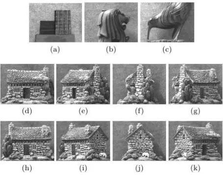
between the DfD results before and after correction, we have chosen a number of test scenes

as shown in Fig. 7, which comprise one with two wooden staircases(Stair), a wooden lion

stature(Lion), a wooden bird stature(Bird) and eight views of a stone house model(House).

Subbarao’s, Favaro’s, Raj’s and Li’s methods are used to compare results before and after

corrections.

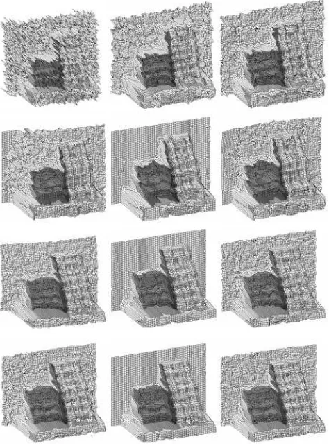
Fig. 8 shows the results of Stair before and after correction for the four DfD methods. The

uncorrected result of Subbarao’s method in row 1 shows heavy spike-like noises throughout

the plot, which are sufficiently severe that the global elliptical deformation centred at the

bottom right part of the plot is hardly visible. After correction, the noises are considerable

reduced and the deformation is also removed. In the uncorrected result of Favaro’s method in

row 2, the deformation is more visible in the background, which is removed after correction.

In the uncorrected result of the Raj’s method in row 3, the deformation is visible in both the

background and foreground, which is effectively removed after correction. In the uncorrected

result of the Li’s method in row 4, the deformation is not visible and the correction methods

make no significant changes to the reconstruction. Furthermore, for all these methods, CDC

produces lower noise levels than CLSF.

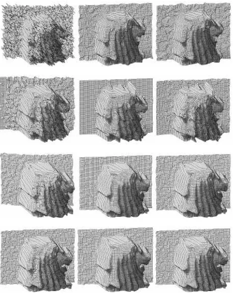
Fig. 9 shows the results of Lion before and after correction. The spike-like noises

through-Fig. 7. Test scenes: (a) - (c) near-focused images of Stair, Lion and Bird, respectively; (d)-(k)

Fig. 8. Wire-frame plots of Stair: row 1-4: Subbarao, Favaro, Raj, and Li. Column 1: Original;

column 2: corrected using CDC; column 3: corrected using CLSF.

out the plot of the uncorrected result of the Subbarao’s method in row 1 are effectively

reduced after correction. In the uncorrected result of the Favaro’s method in row 2, a small

deformation in the background makes the left part further away than the right. The

defor-mation is reduced after correction. Moreover, CDC produces lower noise level than CLSF.

In the uncorrected result of the Raj’s method in row 3, a strong elliptical deformation in the

background makes the top-left corner further away than it should be. The deformation also

appears at the front of the house. The deformation is significantly reduced after correction.

In addition, CDC produces lower noise level than CLSF. In the uncorrected result of the

Li’s method in row 4, a small deformation in the background, makes the top right slightly

closer than it should be. The deformation is removed after correction.

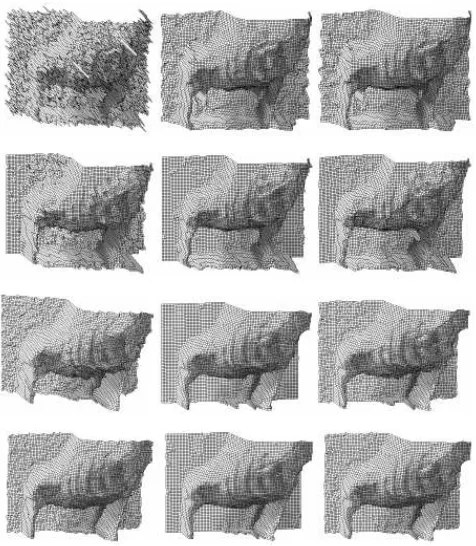
Fig. 10 shows the results of Bird before and after correction. In the uncorrected result

of the Subbarao’s method in row 1, the spike-like noise is present throughout the plot. The

Fig. 9. Wire-frame plots of Lion: row 1-4: Subbarao, Favaro, Raj, and Li. Column 1: Original;

column 2: corrected using CDC; column 3: corrected using CLSF.

body. These artefacts are effectively reduced after correction. In the uncorrected result of

the Favaro’s method in row 2, no significant deformation is visible since the right part of the

flat background is mostly occluded by the bird. However, the poor reconstruction makes it

difficult to determine whether the bottom right corner of the plot is the bird or the

back-ground. After correction, it is clear that the bottom right corner is part of the backback-ground.

The quality of the reconstruction is also considerably improved as a result. In the

uncor-rected result of the Raj’s method in row 3, a strong deformation makes the background not

flat and the reconstruction of the bird is poor. After correction, the background is made

flat and the reconstruction is improved. CDC also produces smaller noise level than CLSF.

In the uncorrected result of the Li’s method in row 4, no significant deformation is visible.

Thus, no significant changes are made to the reconstruction after correction, except CDC

reduces the local noises.

Fig. 11 shows the results of eight views of House using Li’s method corrected by CDC.

Fig. 10. Bird: row 1-4: Subbarao, Favaro, Raj, and Li. Column 1: Original; column 2: corrected

using CDC; column 3: corrected using CLSF.

bumpy, no spike-like noise and elliptical deformation are visible. Overall, these plots show

that CDC produces good quality reconstructions for House.

As the experimental results illustrate, both CDC and CLSF are able to eliminate the

elliptical deformation effectively. In combination with the post-processing algorithm, both

methods significantly mitigate the unstable depth results due to low-texture regions. CDC

improves the smoothness of the flat and smooth surfaces. However, it is complex which

involves a number of iterative searching procedures. CLSF is very efficient with a closed

form equation in Eqn. (12). However it produces coarser correction result than CDC.

Note that since the DfD method in [19] is already incorporated with a correction algorithm

which removes most deformation, the qualitative results in Fig. 8 - Fig. 10 show little

improvement compared to other methods. However, this does not mean the DfD method in

[19] is good in all cases. For example, in Fig. 8, there is significant amount of noise in the

background flat surface which is effectively mitigated after correction, especially with CDC.

In addition, the quantitative results in Section 6.B also show that CDC and CLSF provide

Fig. 11. Wire-frame plots of eight views of the house using Li’s method after CDC.

6.D. Computational cost

In terms of processing time taken to correct a 63×86 depth map, CDC requires 994

mil-liseconds and CLSF requires 5.87 milmil-liseconds without post-processing. The additional 443

milliseconds is typically required for the post-processing. Thus, CLSF is faster than CDC

at a cost of lower accuracy and smoothness. The correction method in [19] which does not

involve post-processing takes 10.3 milliseconds. Note that serial implementations are used

to estimate the speed. Thus, parallel implementations are theoretically able to decrease the

computational costs, since all pixels can be processed separately.

7. Conclusion

This paper presents two DfD correction methods to address the depth-variant elliptical

deformation that often occurs during DfD computation. The methods correct the depth

estimation generated by any DfD algorithm using a number of correction patterns generated

by the correction method. CDC finds the nearest CPV to cancel out the deformation at

every location and further improves the accuracy with consideration of the local region and

interpolation. CLSF finds the mapping from the deformed to the corrected results directly

sharing separate sets of coefficients. CDC produces better reconstructions than CLSF but

at the expense of much lower speed. Both quantitative and qualitative experiments on real

images show that the proposed methods effectively remove the deformation and other noise.

Since this paper is on passive DfD using two input images, in the future, we will explore

the applicability of both CDC and CLSF on DfD using a single image and those techniques

assisted by active pattern projection, i.e. active DfD. In addition, we plan to investigate

modelling techniques that are more sophisticated than least squares fit to further improve

the reconstruction accuracy. Furthermore, we will consider machine learning techniques for

deformation removal.

8. Acknowledgement

We would like to thank Warwick Engineering Bursary for providing the research fund.

References

[1] A. P. Pentland, “A new sense for depth of field”, IEEE Transactions on Pattern Analysis and

Machine Intelligence 9, 523-531 (1987).

[2] A. P. Pentland, “A simple, real-time range camera”, in Proceedings of IEEE Conference on

Computer Vision and Pattern Recognition (IEEE,1989) pp. 256-261.

[3] M. Subbarao, “Parallel depth recovery by changing camera parameters”, in Proceedings of

IEEE ICCV (IEEE, 1988), pp. 149-155.

[4] A. N. Rajagopalan and S. Chaudhuri, “An MRF model-based approach to simultaneous

recov-ery of depth and restoration from defocused images”, IEEE Transactions on Pattern Analysis

and Machine Intelligence 21, 577-589 (1999).

[5] J. Ens and P. Lawrence, “An investigation of methods for determining depth from focus”,

IEEE Transactions on Pattern Analysis and Machine Intelligence 15, 97-108 (1987).

[6] V. Michael Bove, “Entropy-based depth from focus”, Journal of the Optical Society of America

A 10, 561-566 (1993).

[7] Ambasamudram N. Rajagopalan and Subhasis Chaudhuri, “Space-variant approaches to

309-329 (1997).

[8] M. Watanabe and S. K. Nayar, “Rational filters for passive depth from defocus”, International

Journal of Computer Vision 27, 203-225 (1998).

[9] A. N. J. Raj and R. C. Staunton, “Rational filter design for depth from defocus”, Pattern

Recognition 45, 198-207 (2012).

[10] P. Favaro and S. Soatto, “Learning shape from defocus”, in Proceedings of 7th European

Conference on Computer Vision (Springer, 2002) pp. 735-745.

[11] Chandramouli Paramanand and Ambasamudram N. Rajagopalan, “Depth from motion and

optical blur with an unscented kalman filter”, IEEE Transactions on Image Processing 21,

2798-2811 (2012).

[12] A. Levin, R. Fergus, F. Durand, “Image and depth from a conventional camera with a coded

aperture,” ACM Transactions on Graphics (TOG) 26, 70 (2007).

[13] C. Zhou, S. Lin and S. Nayar, “Coded aperture pairs for depth from defocus and defocus

deblurring,” Int. J. Comput. Vis 93, 53-72 (2011).

[14] H. Wang, F. Cao, S. Fang, et al., “Effective improvement for depth estimated based on defocus

images,” Journal of Computers 8, 888-895 (2013).

[15] Q. F. Wu, K. Q. Wang, and W. M. Zuo, “Depth from defocus using geometric optics

regular-ization,” Advanced Materials Research 709, 511-514 (2013).

[16] S. F. Ray, Applied Photographic Optics: Imaging Systems for Photography, Film and Video

(Focal Press, 1988).

[17] Julie Bentley and Craig Olson, Field Guide to Lens Design (SPIE Press, 2012).

[18] Hari N. Nair and Charles V Stewart, “Robust focus ranging”, in Proceedings of IEEE

Con-ference on Computer Vision and Pattern Recognition, (IEEE, 1992) pp. 309-314.

[19] Ang Li, Richard Staunton and Tardi Tjahjadi, “Rational-operator-based depth-from-defocus

approach to scene reconstruction”, Journal of the Optical Society of America A30, 1787-1795

(2013).

[20] Rafael C. Gonzalez, Richard Eugene Woods and Steven L. Eddins, Digital Image Processing

Using MATLAB (Pearson Prentice Hall, 2004).

[21] M. Watanabe and S. K. Nayar, “Telecentric optics for focus analysis,” IEEE Transactions on