Worst case and probabilistic analysis of the 2 Opt algorithm for the TSP

http://wrap.warwick.ac.uk

Original citation:

Englert, Matthias, Röglin, Heiko and Vöcking, Berthold. (2014) Worst case and

probabilistic analysis of the 2-Opt algorithm for the TSP. Algorithmica, Volume 68

(Number 1). pp. 190-264. ISSN 0178-4617

Permanent WRAP url:

http://wrap.warwick.ac.uk/59263

Copyright and reuse:

The Warwick Research Archive Portal (WRAP) makes this work of researchers of the

University of Warwick available open access under the following conditions.

This article is made available under the Creative Commons Attribution 3.0 (CC BY 3.0)

license and may be reused according to the conditions of the license. For more details

see: http://creativecommons.org/licenses/by/3.0/

A note on versions:

The version presented in WRAP is the published version, or, version of record, and may

be cited as it appears here.

DOI 10.1007/s00453-013-9801-4

Worst Case and Probabilistic Analysis of the 2-Opt

Algorithm for the TSP

Matthias Englert·Heiko Röglin· Berthold Vöcking

Received: 25 January 2008 / Accepted: 6 June 2013 / Published online: 19 June 2013 © Springer Science+Business Media New York 2013

Abstract 2-Opt is probably the most basic local search heuristic for the TSP. This

heuristic achieves amazingly good results on “real world” Euclidean instances both with respect to running time and approximation ratio. There are numerous exper-imental studies on the performance of 2-Opt. However, the theoretical knowledge about this heuristic is still very limited. Not even its worst case running time on 2-dimensional Euclidean instances was known so far. We clarify this issue by present-ing, for everyp∈N, a family ofLpinstances on which 2-Opt can take an exponential number of steps.

Previous probabilistic analyses were restricted to instances in whichnpoints are placed uniformly at random in the unit square[0,1]2, where it was shown that the expected number of steps is bounded byO(n˜ 10)for Euclidean instances. We con-sider a more advanced model of probabilistic instances in which the points can be placed independently according to general distributions on[0,1]d, for an arbitrary d≥2. In particular, we allow different distributions for different points. We study the expected number of local improvements in terms of the numbernof points and the maximal densityφof the probability distributions. We show an upper bound on the expected length of any 2-Opt improvement path ofO(n˜ 4+1/3·φ8/3). When starting

An extended abstract appeared in Proc. of the 18th ACM-SIAM Symposium on Discrete Algorithms (SODA 2007).

M. Englert

DIMAP and Dept. of Computer Science, University of Warwick, Coventry, UK e-mail:[email protected]

H. Röglin (

B

Dept. of Computer Science, University of Bonn, Bonn, Germany e-mail:[email protected]

B. Vöcking

with an initial tour computed by an insertion heuristic, the upper bound on the ex-pected number of steps improves even toO(n˜ 4+1/3−1/d·φ8/3). If the distances are measured according to the Manhattan metric, then the expected number of steps is bounded byO(n˜ 4−1/d·φ). In addition, we prove an upper bound ofO(√d_{φ)on the} expected approximation factor with respect to allLpmetrics.

Let us remark that our probabilistic analysis covers as special cases the uniform input model withφ=1 and a smoothed analysis with Gaussian perturbations of stan-dard deviationσ withφ∼1/σd.

Keywords TSP·2-Opt·Probabilistic analysis

1 Introduction

In the traveling salesperson problem (TSP), we are given a set of vertices and for each pair of distinct vertices a distance. The goal is to find a tour of minimum length that visits every vertex exactly once and returns to the initial vertex at the end. Despite many theoretical analyses and experimental evaluations of the TSP, there is still a considerable gap between the theoretical results and the experimental observations. One important special case is the Euclidean TSP in which the vertices are points inRd, for somed∈N, and the distances are measured according to the Euclidean metric. This special case is known to beNP-hard in the strong sense [15], but it admits a polynomial time approximation scheme (PTAS), shown independently in 1996 by Arora [1] and Mitchell [13]. These approximation schemes are based on dynamic programming. However, the most successful algorithms on practical instances rely on the principle of local search and very little is known about their complexity.

The 2-Opt algorithm is probably the most basic local search heuristic for the TSP. 2-Opt starts with an arbitrary initial tour and incrementally improves this tour by making successive improvements that exchange two of the edges in the tour with two other edges. More precisely, in each improving step the 2-Opt algorithm selects two edges{u1, u2}and{v1, v2}from the tour such thatu1, u2, v1, v2are distinct and

appear in this order in the tour, and it replaces these edges by the edges{u1, v1}and

{u2, v2}, provided that this change decreases the length of the tour. The algorithm

terminates in a local optimum in which no further improving step is possible. We use the term 2-change to denote a local improvement made by 2-Opt. This simple heuristic performs amazingly well on “real-life” Euclidean instances like, e.g., the ones in the well-known TSPLIB [17]. Usually the 2-Opt heuristic needs a clearly subquadratic number of improving steps until it reaches a local optimum and the computed solution is within a few percentage points of the global optimum [7].

consider a 2-Opt variant for the Euclidean plane in which only steps are allowed that remove a crossing from the tour. Such steps can introduce new crossings, but van Leeuwen and Schoone [20] show that afterO(n3)steps, 2-Opt finds a tour without any crossing. On the negative side, Lueker [12] constructs TSP instances whose state graphs contain exponentially long paths. Hence, 2-Opt can take an exponential num-ber of steps before it finds a locally optimal solution. This result is generalized to k-Opt, for arbitrary k≥2, by Chandra, Karloff, and Tovey [3]. These negative re-sults, however, use arbitrary graphs that cannot be embedded into low-dimensional Euclidean space. Hence, they leave open the question as to whether it is possible to construct Euclidean TSP instances on which 2-Opt can take an exponential number of steps, which has explicitly been asked by Chandra, Karloff, and Tovey. We resolve this question by constructing such instances in the Euclidean plane. In chip design applications, often TSP instances arise in which the distances are measured accord-ing to the Manhattan metric. Also for this metric and for every otherLpmetric, we construct instances with exponentially long paths in the 2-Opt state graph.

Theorem 1 For every p∈ {1,2,3, . . .} ∪ {∞} and n∈N= {1,2,3, . . .}, there is a two-dimensional TSP instance with 16nvertices in which the distances are mea-sured according to theLp metric and whose state graph contains a path of length 2n+4_−22.

For Euclidean instances in whichnpoints are placed independently uniformly at random in the unit square, Kern [8] shows that the length of the longest path in the state graph is bounded byO(n16)with probability at least 1−c/nfor some con-stantc. Chandra, Karloff, and Tovey [3] improve this result by bounding the expected length of the longest path in the state graph byO(n10logn). That is, independent of the initial tour and the choice of the local improvements, the expected number of 2-changes is bounded byO(n10logn). For instances in whichn points are placed uniformly at random in the unit square and the distances are measured according to the Manhattan metric, Chandra, Karloff, and Tovey show that the expected length of the longest path in the state graph is bounded byO(n6logn).

analysis, in which first an adversary specifies the positions of the points and after that each position is slightly perturbed by adding a Gaussian random variable with small standard deviationσ. In this case, one has to setφ=1/(√2π σ )d.

We prove the following theorem about the expected length of the longest path in the 2-Opt state graph for the three probabilistic input models discussed above. It is assumed that the dimensiond≥2 is an arbitrary constant.

Theorem 2 The expected length of the longest path in the 2-Opt state graph

(a) isO(n4·φ)forφ-perturbed Manhattan instances withnpoints.

(b) isO(n4+1/3·log(nφ)·φ8/3)forφ-perturbed Euclidean instances withnpoints.

Usually, 2-Opt is initialized with a tour computed by some tour construction heuristic. One particular class is that of insertion heuristics, which insert the vertices one after another into the tour. We show that also from a theoretical point of view, using such an insertion heuristic yields a significant improvement for metric TSP instances because the initial tour 2-Opt starts with is much shorter than the longest possible tour. In the following theorem, we summarize our results on the expected number of local improvements.

Theorem 3 The expected number of steps performed by 2-Opt

(a) isO(n4−1/d·logn·φ)onφ-perturbed Manhattan instances withnpoints when 2-Opt is initialized with a tour obtained by an arbitrary insertion heuristic. (b) isO(n4+1/3−1/d ·log2(nφ)·φ8/3)onφ-perturbed Euclidean instances with n

points when 2-Opt is initialized with a tour obtained by an arbitrary insertion heuristic.

In fact, our analysis shows not only that the expected number of local improve-ments is polynomially bounded but it also shows that the second moment and hence the variance is bounded polynomially forφ-perturbed Manhattan instances. For the Euclidean metric, we cannot bound the variance but the 3/2-th moment polynomially. In [5], we also consider a model in which an arbitrary graphG=(V , E)is given along with, for each edgee∈E, a probability distribution according to which the edge lengthd(e)is chosen independently of the other edge lengths. Again, we restrict the choice of distributions to distributions that can be represented by density functions fe: [0,1] → [0, φ]with maximal density at mostφ for a givenφ≥1. We denote inputs created by this input model asφ-perturbed graphs. Observe that in this input model only the distances are perturbed whereas the graph structure is not changed by the randomization. This can be useful if one wants to explicitly prohibit certain edges. However, if the graphGis not complete, one has to initialize 2-Opt with a Hamiltonian cycle to start with. We prove that in this model the expected length of the longest path in the 2-Opt state graph isO(|E| ·n1+o(1)·φ). As the techniques for proving this result are different from the ones used in this article, we will present it in a separate journal article.

quite negative results on the worst-case behavior of 2-Opt. For example, Chandra, Karloff, and Tovey [3] show that there are Euclidean instances in the plane for which 2-Opt has local optima whose costs areΩ(_{log log}logn_n) times larger than the optimal costs. However, the same authors also show that the expected approximation ratio of the worst local optimum for instances withnpoints drawn uniformly at random from the unit square is bounded from above by a constant. We generalize their result to our input model in which different points can have different distributions with bounded densityφand to allLpmetrics.

Theorem 4 Letp∈N∪ {∞}. Forφ-perturbedLpinstances, the expected approxi-mation ratio of the worst tour that is locally optimal for 2-Opt isO(√d_φ).

The remainder of the paper is organized as follows. We start by stating some basic definitions and notation in Sect.2. In Sect.3, we present the lower bounds. In Sect.4, we analyze the expected number of local improvements and prove Theorems2and3. Finally, in Sects.5and6, we prove Theorem4about the expected approximation factor and we discuss the relation between our analysis and a smoothed analysis.

2 Preliminaries

An instance of the TSP consists of a setV = {v1, . . . , vn}of vertices (depending on the context, synonymously referred to as points) and a symmetric distance function d:V×V →R_≥0that associates with each pair{vi, vj}of distinct vertices a distance

d(vi, vj)=d(vj, vi). The goal is to find a Hamiltonian cycle of minimum length. We also use the term tour to denote a Hamiltonian cycle. We defineN= {1,2,3, . . .}, and for a natural numbern∈N, we denote the set{1, . . . , n}by[n].

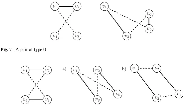
A pair(V ,d)of a nonempty setV and a functiond: V ×V →R_≥0is called a

metric space if for allx, y, z∈V the following properties are satisfied:

(a) d(x, y)=0 if and only ifx=y (reflexivity), (b) d(x, y)=d(y, x)(symmetry), and

(c) d(x, z)≤d(x, y)+d(y, z)(triangle inequality).

If(V ,d)is a metric space, thendis called a metric onV. A TSP instance with vertices V and distance functiondis called metric TSP instance if(V ,d)is a metric space.

A well-known class of metrics onRd is the class ofLp metrics. Forp∈N, the distance dp(x, y) of two points x ∈Rd andy ∈Rd with respect to the Lp met-ric is given bydp(x, y)= p

√

|x1−y1|p+ · · · + |xd−yd|p. TheL1metric is often

called Manhattan metric, and theL2metric is well-known as Euclidean metric. For p→ ∞, theLpmetric converges to theL∞metric defined by the distance function

d_∞(x, y)=max{|x1−y1|, . . . ,|xd−yd|}. A TSP instance(V ,d)withV ⊆Rd in whichd equalsdp restricted to V is called anLp instance. We also use the terms Manhattan instance and Euclidean instance to denoteL1andL2instances,

respec-tively. Furthermore, ifpis clear from context, we writedinstead ofdp.

is used as the initial solution 2-Opt starts with. A well-known class of tour con-struction heuristics for metric TSP instances are so-called insertion heuristics. These heuristics insert the vertices into the tour one after another, and every vertex is in-serted between two consecutive vertices in the current tour where it fits best. To make this more precise, letTi denote a subtour on a subset Si ofivertices, and suppose v /∈Si is the next vertex to be inserted. If(x, y)denotes an edge inTithat minimizes

d(x, v)+d(v, y)−d(x, y), then the new tourTi₊1is obtained fromTiby deleting the

edge(x, y)and adding the edges(x, v)and(v, y). Depending on the order in which the vertices are inserted into the tour, one distinguishes between several different in-sertion heuristics. Rosenkrantz et al. [18] show an upper bound oflogn +1 on the approximation factor of any insertion heuristic on metric TSP instances. Furthermore, they show that two variants which they call nearest insertion and cheapest insertion achieve an approximation ratio of 2 for metric TSP instances. The nearest insertion heuristic always inserts the vertex with the smallest distance to the current tour (i.e., the vertexv /∈Sithat minimizes minx∈Sid(x, v)), and the cheapest insertion heuristic always inserts the vertex whose insertion leads to the cheapest tourTi₊1.

3 Exponential Lower Bounds

In this section, we answer Chandra, Karloff, and Tovey’s question [3] as to whether it is possible to construct TSP instances in the Euclidean plane on which 2-Opt can take an exponential number of steps. We present, for everyp∈N∪ {∞}, a family of two-dimensional Lp instances with exponentially long sequences of improving 2-changes. In Sect.3.1, we present our construction for the Euclidean plane, and in Sect.3.2we extend this construction to generalLpmetrics.

3.1 Exponential Lower Bound for the Euclidean Plane

In Lueker’s construction [12] many of the 2-changes remove two edges that are far apart in the current tour in the sense that many vertices are visited between them. Our construction differs significantly from the previous one as the 2-changes in our construction affect the tour only locally. The instances we construct are composed of gadgets of constant size. Each of these gadgets has a zero state and a one state, and there exists a sequence of improving 2-changes starting in the zero state and even-tually leading to the one state. LetG0, . . . , Gn−1denote these gadgets. If gadgetGi withi >0 has reached state one, then it can be reset to its zero state by gadgetGi₋1.

The crucial property of our construction is that whenever a gadgetGi−1changes its

state from zero to one, it resets gadgetGi twice. Hence, if in the initial tour, gadget G0is in its zero state and every other gadget is in state one, then for every iwith

0≤i≤n−1, gadgetGi performs 2i _{state changes from zero to one as, fori >0,} gadgetGi is reset 2itimes.

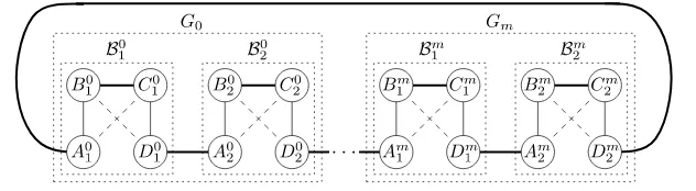
Fig. 1 In the illustration, we usemto denoten−1. Every tour that occurs in the sequence of 2-changes contains the thick edges. For each block, either both solid or both dashed edges are contained. In the former case the block is in its short state; in the latter case the block is in its long state

construction ensures the following property: The pointsAi_j,B_ji,C_ji, andD_ji are al-ways visited consecutively in the tour either in the orderAi_jB_jiCi_jD_ji or in the or-derAi_jC_jiB_jiDi_j.

Observe that the change from one of these configurations to the other corresponds to a single 2-change in which the edgesAi_jB_ji andCi_jD_ji are replaced by the edges Ai_jC_ji andB_jiDi_j, or vice versa. In the following, we assume that the sumd(Ai_j, B_ji)+

d(C_ji, D_ji)is strictly smaller than the sumd(Ai_j, C_ji)+d(B_ji, Di_j), and we refer to the

configurationAi_jB_jiC_jiD_ji as the short state of the block and to the configuration Ai_jC_jiB_jiDi_jas the long state. Another property of our construction is that neither the order in which the blocks are visited nor the order of the gadgets is changed during the sequence of 2-changes. Again with the exception of the intermediate configurations, the order in which the blocks are visited isB0₁B₂0B1₁B1₂· · ·B₁n−1Bn₂−1(see Fig.1).

Due to the aforementioned properties, we can describe every non-intermediate tour that occurs during the sequence of 2-changes completely by specifying for every block if it is in its short state or in its long state. In the following, we denote the state of a gadgetGiby a pair(x1, x2)withxj∈ {S, L}, meaning that blockBji is in its short state if and only ifxj=S. Since every gadget consists of two blocks, there are four possible states for each gadget. However, only three of them appear in the sequence of 2-changes, namely(L, L),(S, L), and(S, S). We call state(L, L)the zero state and state(S, S)the one state. In order to guarantee the existence of an exponentially long sequence of 2-changes, the gadgets we construct possess the following property.

Property 5 If, fori∈ {0, . . . , n−2}, gadgetGi is in state(L, L)(or(S, L), respec-tively) and gadgetGi₊1is in state(S, S), then there exists a sequence of seven

con-secutive 2-changes terminating with gadgetGi being in state(S, L)(or state(S, S), respectively) and gadgetGi₊1 in state (L, L). In this sequence only edges of and

between the gadgetsGi andGi+1are involved.

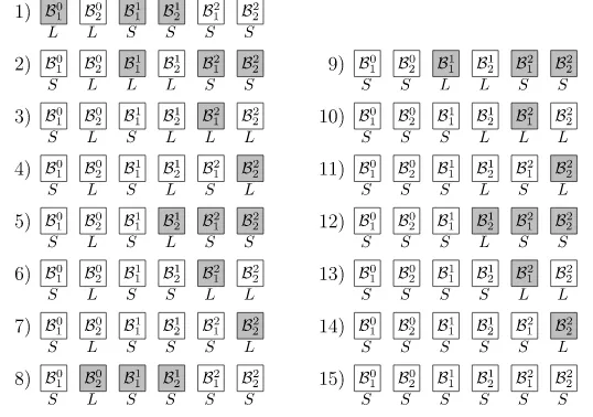
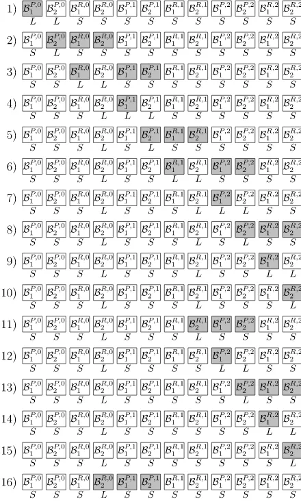
Fig. 2 This figure shows an example with three gadgets. It shows the 15 configurations that these gadgets assume during the sequence of 2-changes, excluding the intermediate configurations that arise when one gadget resets another one. Gadgets that are involved in the transformation from configurationito configu-rationi+1 are shown in gray. For example, in the step from the first to the second configuration, the first blockB0₁of gadgetG0resets the two blocks of gadgetG1. That is, these three blocks follow the sequence

of seven 2-changes from Property5. On the other hand, in the step from the third to the fourth config-uration only the first blockB2₁of gadgetG2is involved. It changes from its long state to its short state

by a single 2-change. As this figure shows an example with three gadgets, the total number of 2-changes performed according to Lemma6is 23+3−0−14=50. This is indeed the case because 6 of the 14 shown steps correspond to sequences of seven 2-changes while 8 steps correspond to single 2-changes

zero to state one, as the following lemma shows. An example with three gadgets is also depicted in Fig.2.

Lemma 6 If, fori∈ {0, . . . , n−1}, gadgetGi is in the zero state(L, L)and all gadgetsGj withj > i are in the one state (S, S), then there exists a sequence of 2n+3−i−14 consecutive 2-changes in which only edges of and between the gadgets Gj withj≥iare involved and that terminates in a state in which all gadgetsGj withj ≥iare in the one state(S, S).

Proof We prove the lemma by induction oni. If gadget Gn₋1 is in state (L, L),

then it can change its state with two 2-changes to (S, S) without affecting the other gadgets. This is true because the two blocks of gadget Gn₋1 can, one

after another, change from their long state An_j−1C_jn−1B_jn−1Dn_j−1 to their short state An_j−1B_jn−1C_jn−1D_jn−1 by a single 2-change. Hence, the lemma is true for i=n−1 because 2n+3−(n−1)−14=2.

of(2n+2−i−14)2-changes after which all gadgetsGj withj > iare in state(S, S). Then, due to Property5, there exists a sequence of seven consecutive 2-changes in which onlyGi changes its state from(S, L)to(S, S)while resetting gadgetGi+1

again from(S, S) to(L, L). Hence, we can apply the induction hypothesis again, yielding that after another(2n+2−i _{−14)2-changes all gadgets Gj withj ≥i are} in state(S, S). This concludes the proof as the number of 2-changes performed is

14+2(2n+2₋i₋₁₄₎₌₂n+3₋i_−14.

In particular, this implies that, given Property5, one can construct instances con-sisting of 2n gadgets, i.e., 16n points, whose state graphs contain paths of length 22n+3_−14>2n+4_{−22, as desired in Theorem1.}

3.1.1 Detailed Description of the Sequence of Steps

Now we describe in detail how a sequence of 2-changes satisfying Property5 can be constructed. First, we assume that gadgetGi is in state(S, L) and that gadget Gi₊1 is in state(S, S). Under this assumption, there are three consecutive blocks,

namelyBi₂,B₁i+1, and Bi₂+1, such that the leftmost oneBi₂is in its long state, and the other blocks are in their short states. We need to find a sequence of 2-changes in which only edges of and between these three blocks are involved and after whichB₂i is in its short state and the other blocks are in their long states. Remember that when the edges{u1, u2}and{v1, v2}are removed from the tour and the vertices appear in

the orderu1, u2, v1, v2 in the current tour, then the edges{u1, v1}and{u2, v2}are

added to the tour and the subtour betweenu1 andv2is visited in reverse order. If,

e.g., the current tour corresponds to the permutation(1,2,3,4,5,6,7)and the edges

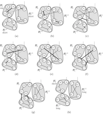
{1,2}and{5,6}are removed, then the new tour is(1,5,4,3,2,6,7). The following sequence of 2-changes, which is also shown in Fig.3, has the desired properties. Brackets indicate the edges that are removed from the tour.

Long state ACBD Short state ABCD Short state ABCD (1) [Ai₂ Ci₂] B₂i D₂i Ai₁+1 B₁i+1 C₁i+1 D₁i+1 Ai₂+1 B₂i+1 [C₂i+1 Di₂+1] (2) Ai₂ C₂i+1 [B₂i+1 Ai₂+1] Di₁+1 C₁i+1 B₁i+1 Ai₁+1 [D₂i B₂i] C₂i Di₂+1 (3) Ai₂ C₂i+1 [B₂i+1 D₂i] Ai₁+1 B₁i+1 [C₁i+1 Di₁+1] Ai₂+1 B₂i C₂i Di₂+1 (4) Ai₂ C₂i+1 B₂i+1 C₁i+1 [B₁i+1 A₁i+1] Di₂ Di₁+1 A₂i+1 B₂i [C₂i Di₂+1] (5) [Ai₂ C₂i+1] B₂i+1 C₁i+1 B₁i+1 C₂i [B₂i Ai₂+1] D₁i+1 D₂i Ai₁+1 Di₂+1 (6) Ai₂ Bi₂ C₂i B₁i+1 [C₁i+1 B₂i+1] C₂i+1 Ai₂+1 D₁i+1 D₂i [Ai₁+1 Di₂+1] (7) Ai₂ Bi₂ [C₂i B₁i+1] C₁i+1 Ai₁+1 [D₂i Di₁+1] Ai₂+1 C₂i+1 B₂i+1 Di₂+1

Ai₂ Bi₂ C₂i D₂i Ai₁+1 C₁i+1 B₁i+1 Di₁+1 Ai₂+1 C₂i+1 B₂i+1 Di₂+1 Short state ABCD Long state ACBD Long state ACBD

Fig. 3 This figure shows the sequence of seven consecutive 2-changes from Property5. In each step the

thick edges are removed from the tour, and the dotted edges are added to the tour. It shows how block Bi

2switches from its long to its short state while resetting the blocksBi1+1andBi2+1from their short to

their long states. This figure is only schematic and it does not show the actual geometric embedding of the points into the Euclidean plane

configurations 2 to 7 are exactly the intermediate configurations that we mentioned at the beginning of this section.

3.1.2 Embedding the Construction into the Euclidean Plane

The only missing step in the proof of Theorem1 for the Euclidean plane is to find points such that all of the 2-changes that we described in the previous section are improving. We specify the positions of the points of gadgetGn−1 and give a rule

as to how the points of gadgetGi can be derived when all points of gadgetGi+1

have already been placed. In our construction it happens that different points have exactly the same coordinates. This is only for ease of notation; if one wants to obtain a TSP instance in which distinct points have distinct coordinates, one can slightly move these points without affecting the property that all 2-changes are improving.

For j ∈ [2], we choose An_j−1 =(0,0), B_jn−1 =(1,0), C_jn−1 =(−0.1,1.4), and Dn_j−1 = (−1.1,4.8). Then A_jn−1B_jn−1C_jn−1D_jn−1 is the short state and An_j−1Cn_j−1B_jn−1Dn_j−1is the long state because

dAn_j−1, C_jn−1+dB_jn−1, Dn_j−1>dAn_j−1, B_jn−1+dC_jn−1, D_jn−1, as

dAn_j−1, C_jn−1+dB_jn−1, Dn_j−1=

0.12_+1.42_+2.12_+4.82_>6.64

and

dAn_j−1, B_jn−1+dCn_j−1, D_jn−1=12₊₀2₊₁2_+3.42_<4.55.

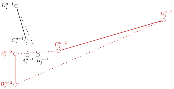
We place the points of gadgetGi as follows (see Fig.4):

1. Start with the coordinates of the points of gadgetGi₊1.

2. Rotate these points around the origin by 3π/2. 3. Scale each coordinate by a factor of 3. 4. Translate the points by the vector(−1.2,0.1).

Fig. 4 This illustration shows the points of the gadgetsGn−1andGn−2. One can see thatGn−2is a

Forj∈ [2], this yieldsAn_j−2=(−1.2,0.1),B_jn−2=(−1.2,−2.9),Cn_j−2=(3,0.4), andD_jn−2=(13.2,3.4).

From this construction it follows that each gadget is a scaled, rotated, and trans-lated copy of gadgetGn−1. If one has a set of points in the Euclidean plane that

admits certain improving 2-changes, then these 2-changes are still improving if one scales, rotates, and translates all points in the same manner. Hence, it suffices to show that the sequences in which gadgetGn−2resets gadgetGn−1from(S, S)to(L, L)

are improving because, for anyi, the points of the gadgetsGi andGi+1are a scaled,

rotated, and translated copy of the points of the gadgetsGn−2andGn−1.

There are two sequences in which gadgetGn−2resets gadgetGn−1from(S, S)to (L, L): in the first one, gadgetGn−2changes its state from(L, L)to(S, L), in the

second one, gadgetGn−2changes its state from(S, L)to(S, S). Since the

coordi-nates of the points in both blocks of gadgetGn−2are the same, the inequalities for

both sequences are also identical. The following inequalities show that the improve-ments made by the steps in both sequences are all positive (see Fig.3or the table in Sect.3.1.1for the sequence of 2-changes):

(1) dAn₂−2, C₂n−2+dC₂n−1, Dn₂−1−dA₂n−2, C₂n−1−dC₂n−2, Dn₂−1>0.03, (2) dB₂n−1, An₂−1+dD₂n−2, B₂n−2−dB₂n−1, Dn₂−2−dA₂n−1, B₂n−2 >0.91, (3) dB₂n−1, D₂n−2+dC₁n−1, Dn₁−1−dB₂n−1, C₁n−1−dD₂n−2, D₁n−1>0.06, (4) dB₁n−1, An₁−1+dC₂n−2, Dn₂−1−dB₁n−1, C₂n−2−dA₁n−1, D₂n−1>0.05, (5) dAn₂−2, C₂n−1+dB₂n−2, An₂−1 −dA₂n−2, B₂n−2−dC₂n−1, An₂−1 >0.43, (6) dC₁n−1, B₂n−1+dAn₁−1, Dn₂−1−dC₁n−1, An₁−1−dB₂n−1, Dn₂−1>0.06, (7) dC₂n−2, B₁n−1+dD₂n−2, D₁n−1−dC₂n−2, Dn₂−2−dB₁n−1, Dn₁−1>0.53. This concludes the proof of Theorem1for the Euclidean plane as it shows that all 2-changes in Lemma6are improving.

3.2 Exponential Lower Bound forLpMetrics

inequalities. Instead ofngadgets, our construction consists of 2ngadgets, namelyn propagation gadgetsGP₀, . . . , GP_n−1andnreset gadgetsGR₀, . . . , GR_n−1. The order in which these gadgets appear in the tour isGP₀GR₀GP₁G₁R. . . GP_n−1GR_n−1.

As before, every gadget consists of two blocks and the order in which the blocks and the gadgets are visited does not change during the sequence of 2-changes. Con-sider a reset gadgetGR_i and its neighboring propagation gadgetGP_i+1. We will embed the points of the gadgets into the Manhattan plane in such a way that Property5is still satisfied. That is, ifGR_i is in state(L, L)(or state(S, L), respectively) andGP_i+1 is in state(S, S), then there exists a sequence of seven consecutive 2-changes reset-ting gadgetGP_i+1 to state(L, L) and leaving gadgetGR_i in state (S, L)(or (S, S), respectively). The situation is different for a propagation gadgetGP_i and its neigh-boring reset gadgetGR_i . In this case, ifGP_i is in state(L, L), it first changes its state with a single 2-change to(S, L). After that, gadgetGP_i changes its state to(S, S) while resetting gadgetGR_i from state(S, S)to state(L, L)by a sequence of seven consecutive 2-changes. In both cases, the sequences of 2-changes in which one block changes from its long to its short state while resetting two blocks of the neighboring gadget from their short to their long states are chosen analogously to the ones for the Euclidean plane described in Sect.3.1.1. An example with three propagation and three reset gadgets is shown in Fig.5.

In the initial tour, only gadgetGP₀ is in state(L, L)and every other gadget is in state (S, S). With similar arguments as for the Euclidean plane, we can show that gadgetGR_i is reset from its one state(S, S)to its zero state(L, L)2i times and that the total number of steps is 2n+4_−22.

3.2.1 Embedding the Construction into the Manhattan Plane

As in the construction in the Euclidean plane, the points in both blocks of a re-set gadgetGR_i have the same coordinates. Also in this case one can slightly move all the points without affecting the inequalities if one wants distinct coordinates for distinct points. Again, we choose points for the gadgets GP_n−1 and GR_n−1 and describe how the points of the gadgets GP_i and GR_i can be chosen when the points of the gadgetsGP_i+1 and G_iR₊₁ are already chosen. For j ∈ [2], we choose A_R,jn−1=(0,1),B_R,jn−1=(0,0),C_R,jn−1=(−0.7,0.1), andD_R,jn−1=(−1.2,0.08). Fur-thermore, we choose An_{P ,}−₁1=(−2,1.8), B_{P ,}n−₁1=(−3.3,2.8), C_{P ,}n−₁1=(−1.3,1.4), Dn_{P ,}−₁1=(1.5,0.9), An_{P ,}−₂1=(−0.7,1.6), B_{P ,}n−₂1=(−1.5,1.2),Cn_{P ,}−₂1=(1.9,−1.5), andD_{P ,}n−₂1=(−0.8,−1.1).

Before we describe how the points of the other gadgets are chosen, we first show that the 2-changes within and between the gadgetsGP_n−1andGR_n−1are improving. Forj∈ [2],An_R,j−1B_R,jn−1C_R,jn−1Dn_R,j−1is the short state because

dAn_R,j−1, C_R,jn−1+dB_R,jn−1, D_R,jn−1−dAn_R,j−1, B_R,jn−1+dC_R,jn−1, D_R,jn−1

Fig. 5 This figure shows an example with three propagation and three reset gadgets. It shows the first 16 configurations that these gadgets assume during the sequence of 2-changes, excluding the intermediate configurations that arise when one gadget resets another one. Gadgets that are involved in the transformation from

configurationito

configurationi+1 are shown in

gray. For example, in the step

from the first to the second configuration, the first block

BP ,0

1 of the first propagation

gadgetGP₀ switches from its long to its short state by a single 2-change. Then in the step from the second to the third configuration, the second block

BP ,0

2 of the first propagation

gadgetGP₀ resets the two blocks of the first reset gadgetGR₀. That is, these three blocks follow the sequence of seven 2-changes from Property5

In the 2-change in which GP_n−1 changes its state from (L, L) to (S, L) the edges An_{P ,}−₁1, C_{P ,}n−₁1 and B_{P ,}n−₁1, D_{P ,}n−₁1 are replaced with the edges An_{P ,}−₁1, B_{P ,}n−₁1 and C_{P ,}n−₁1, D_{P ,}n−₁1. This 2-change is improving because

dAn_{P ,}−₁1, C_{P ,}n−₁1+dB_{P ,}n−₁1, D_{P ,}n−₁1−dAn_{P ,}−₁1, B_{P ,}n−₁1+dC_{P ,}n−₁1, D_{P ,}n−₁1

=(0.7+0.4)+(4.8+1.9)−(1.3+1)−(2.8+0.5)=2.2.

The 2-changes in the sequence in whichGP_n−1changes its state from(S, L)to(S, S) while resettingGR_n−1 are chosen analogously to the ones shown in Fig.3 and in the table in Sect.3.1.1. The only difference is that the involved blocks are notBi₂,

Bi+1 1 , andB

i+1

2 anymore, but the second block of gadgetGPn−1and the two blocks of

the improvements made by the 2-changes in this sequence are all positive:

(1) dA_{P ,}n−₂1, C_{P ,}n−₂1+dCn_R,−₂1, Dn_R,−₂1−dA_{P ,}n−₂1, C_R,n−₂1−dC_{P ,}n−₂1, Dn_R,−₂1=0.04, (2) dB_R,n−₂1, An_R,−₂1+dD_{P ,}n−₂1, B_{P ,}n−₂1−dB_R,n−₂1, D_{P ,}n−₂1−dA_R,n−₂1, B_{P ,}n−₂1 =0.4, (3) dB_R,n−₂1, D_{P ,}n−₂1+dCn_R,−₁1, Dn_R,−₁1−dB_R,n−₂1, C_R,n−₁1−dD_{P ,}n−₂1, D_R,n−₁1=0.04, (4) dB_R,n−₁1, An_R,−₁1+dCn_{P ,}−₂1, Dn_R,−₂1−dB_R,n−₁1, C_{P ,}n−₂1−dA_R,n−₁1, D_R,n−₂1=0.16, (5) dA_{P ,}n−₂1, C_R,n−₂1+dB_{P ,}n−₂1, An_R,−₂1 −dA_{P ,}n−₂1, B_{P ,}n−₂1−dC_R,n−₂1, An_R,−₂1 =0.4, (6) dC_R,n−₁1, B_R,n−₂1+dAn_R,−₁1, Dn_R,−₂1−dC_R,n−₁1, An_R,−₁1−dB_R,n−₂1, Dn_R,−₂1=0.04, (7) dC_{P ,}n−₂1, B_R,n−₁1+dD_{P ,}n−₂1, D_R,n−₁1−dC_{P ,}n−₂1, D_{P ,}n−₂1−dB_R,n−₁1, Dn_R,−₁1=0.6.

Again, our construction possesses the property that each pair of gadgetsGP_i and GR_i is a scaled and translated version of the pair GP_n−1 andGR_n−1. Since we have relaxed the requirements for the gadgets, we do not even need rotations here. We place the points ofGP_i andGR_i as follows:

1. Start with the coordinates specified for the points of gadgetsGP_i+1andGR_i+1. 2. Scale each coordinate by a factor of 7.7.

3. Translate the points by the vector(1.93,0.3).

For j ∈ [2], this yields A_R,jn−2 =(1.93,8), B_R,jn−2=(1.93,0.3), C_R,jn−2=(−3.46, 1.07), andD_R,jn−2=(−7.31,0.916). Additionally, it yieldsAn_{P ,}−₁2=(−13.47,14.16), B_{P ,}n−₁2=(−23.48,21.86),C_{P ,}n−₁2=(−8.08,11.08), Dn_{P ,}−₁2=(13.48,7.23),An_{P ,}−₂2= (−3.46,12.62), B_{P ,}n−₂2 =(−9.62,9.54), C_{P ,}n−₂2 = (16.56,−11.25), and D_{P ,}n−₂2 = (−4.23,−8.17).

As in our construction for the Euclidean plane, it suffices to show that the se-quences in which gadgetGR_n−2 resets gadget GP_n−1 from(S, S) to(L, L) are im-proving because, for anyi, the points of the gadgetsGR_i andGP_i+1are a scaled and translated copy of the points of the gadgetsGR_n−2andGP_n−1. The 2-changes in these sequences are chosen analogously to the ones shown in Fig.3 and in the table in Sect.3.1.1. The only difference is that the involved blocks are notBi₂,B₁i+1, andBi₂+1 anymore, but one of the blocks of gadgetGR_n−2and the two blocks of gadgetGP_n−1, respectively. As the coordinates of the points in the two blocks of gadgetGR_n−2 are the same, the inequalities for both sequences are also identical. The improvements made by the steps in both sequences are

(5) dA_R,n−₂2, Cn_{P ,}−₂1+dB_R,n−₂2, An_{P ,}−₂1−dA_R,n−₂2, B_R,n−₂2−dC_{P ,}n−₂1, An_{P ,}−₂1=0.06, (6) dC_{P ,}n−₁1, B_{P ,}n−₂1+dAn_{P ,}−₁1, Dn_{P ,}−₂1−dC_{P ,}n−₁1, An_{P ,}−₁1−dB_{P ,}n−₂1, D_{P ,}n−₂1=0.4, (7) dC_R,n−₂2, B_{P ,}n−₁1+dDn_R,−₂2, Dn_{P ,}−₁1−dC_R,n−₂2, D_R,n−₂2−dB_{P ,}n−₁1, Dn_{P ,}−₁1=0.012. This concludes the proof of Theorem1for the Manhattan metric as it shows that all 2-changes are improving.

Let us remark that this also implies Theorem1 for theL_∞ metric because dis-tances with respect to the L_∞ metric coincide with distances with respect to the Manhattan metric if one rotates all points byπ/4 around the origin and scales every coordinate by 1/√2.

3.2.2 Embedding the Construction into GeneralLpMetrics

It is also possible to embed our Manhattan construction into theLpmetric forp∈N withp≥3. Forj∈ [2], we chooseA_R,jn−1=(0,1),B_R,jn−1=(0,0),C_R,jn−1=(3.5,3.7), and D_R,jn−1 =(7.8,−3.2). Moreover, we choose A_{P ,}n−₁1 =(−2.5,−2.4), B_{P ,}n−₁1 = (−4.7,−7.3), C_{P ,}n−₁1=(−8.6,−4.6),D_{P ,}n−₁1=(3.7,9.8),An_{P ,}−₂1=(3.2,2),B_{P ,}n−₂1= (7.2,7.2),C_{P ,}n−₂1=(−6.5,−1.6), andD_{P ,}n−₂1=(−1.5,−7.1). We place the points of GP_i andGR_i as follows:

1. Start with the coordinates specified for the points of gadgetsGP_i+1andGR_i+1. 2. Rotate these points around the origin byπ.

3. Scale each coordinate by a factor of 7.8. 4. Translate the points by the vector(7.2,5.3).

For j ∈ [2], this yields An_R,j−2=(7.2,−2.5), B_R,jn−2=(7.2,5.3), C_R,jn−2=(−20.1,

−23.56), andD_R,jn−2=(−53.64,30.26). Additionally, it yieldsAn_{P ,}−₁2=(26.7,24.02), B_{P ,}n−₁2=(43.86,62.24),C_{P ,}n−₁2=(74.28,41.18),Dn_{P ,}−₁2=(−21.66,−71.14),An_{P ,}−₂2= (−17.76,−10.3), B_{P ,}n−₂2=(−48.96,−50.86), C_{P ,}n−₂2=(57.9,17.78), and Dn_{P ,}−₂2= (18.9,60.68).

It needs to be shown that the distances of these points when measured according to theLp metric for anyp∈Nwithp≥3 satisfy all necessary inequalities, that is, all 16 inequalities that we have verified in the previous section for the Manhattan metric. Let us start by showing that forj∈ [2],An_R,j−1B_R,jn−1C_R,jn−1D_R,jn−1is the short state. For this, we have to prove the following inequality for everyp∈Nwithp≥3:

dp

An_R,j−1, C_R,jn−1+dp

B_R,jn−1, Dn_R,j−1−dp

An_R,j−1, B_R,jn−1+dp

C_R,jn−1, Dn_R,j−1>0

⇐⇒ √p

3.5p_+2.7p₊√p

7.8p_+3.2p₋√p

0p₊₁p₋√p

4.3p_+6.9p_>0. (3.1)

p √

4.3p_+6.9p_−6.9=6.9·

p

1+

4.3 6.9

p

−1

≤6.9·

3

1+

4.3 6.9

3

−1

<0.52. (3.2)

Hence,

p √

3.5p_+2.7p₊√p

7.8p_+3.2p₋√p

0p₊₁p₋√p

4.3p_+6.9p

≥3.5+7.8−1−6.9−0.52>0,

which proves thatAn_R,j−1B_R,jn−1C_R,jn−1D_R,jn−1is the short state for everyp∈Nwithp≥3. Next we argue that also the 2-change in whichGP_n−1changes its state from(L, L) to(S, L) is improving. For this, the following inequality needs to be verified for everyp∈Nwithp≥3:

dAn_{P ,}−₁1, C_{P ,}n−₁1+dB_{P ,}n−₁1, D_{P ,}n−₁1−dAn_{P ,}−₁1, B_{P ,}n−₁1−dC_{P ,}n−₁1, D_{P ,}n−₁1>0

⇐⇒ √p

6.1p_+2.2p₊√p

8.4p_+17.1p₋√p

2.2p_+4.9p₋√p

12.3p_+14.4p_>0.

As before, we obtain forp∈Nwithp≥3

p √

2.2p_+4.9p_−4.9=4.9·

p

1+

2.2 4.9

p

−1

≤4.9·

3

1+

2.2 4.9

3

−1

<0.15

and

p √

12.3p_+14.4p_{−14.4=14.4·}

p

1+

12.3 14.4

p

−1

≤14.4·

3

1+

12.3 14.4

3

−1

<2.53.

This implies forp∈Nwithp≥3

p √

6.1p_+2.2p₊√p

8.4p_+17.1p₋√p

2.2p_+4.9p₋√p

12.3p_+14.4p

≥6.1+17.1−4.9−0.15−14.4−2.53>0,

which proves that the 2-change in whichGP_n−1changes its state from(L, L)to(S, L) is improving for everyp∈Nwithp≥3.

For this we need to verify the following inequalities for everyp∈Nwithp≥3 (ob-serve that these are exactly the same inequalities that we have verified in Sect.3.2.1

for the Manhattan metric):

(1) dp

An_{P ,}−₂1, C_{P ,}n−₂1+dp

C_R,n−₂1, D_R,n−₂1−dp

An_{P ,}−₂1, Cn_R,−₂1−dp

C_{P ,}n−₂1, Dn_R,−₂1>0

⇐⇒ √p

9.7p_+3.6p₊√p

4.3p_+6.9p₋ √p

0.3p_+1.7p₋√p

14.3p_+1.6p_>0,

(2) dp

B_R,n−₂1, An_R,−₂1+dp

D_{P ,}n−₂1, B_{P ,}n−₂1−dp

B_R,n−₂1, D_{P ,}n−₂1−dp

An_R,−₂1, B_{P ,}n−₂1>0

⇐⇒ √p

0.0p_+1.0p₊√p

8.7p_+14.3p₋√p

1.5p_+7.1p₋√p

7.2p_+6.2p_>0,

(3) dp

B_R,n−₂1, Dn_{P ,}−₂1+dp

C_R,n−₁1, Dn_R,−₁1−dp

B_R,n−₂1, C_R,n−₁1−dp

Dn_{P ,}−₂1, Dn_R,−₁1>0

⇐⇒ √p

1.5p_+7.1p₊√p

4.3p_+6.9p₋ √p

3.5p_+3.7p₋√p

9.3p_+3.9p_>0,

(4) dp

B_R,n−₁1, An_R,−₁1+dp

C_{P ,}n−₂1, D_R,n−₂1−dp

B_R,n−₁1, C_{P ,}n−₂1−dp

An_R,−₁1, Dn_R,−₂1>0

⇐⇒ √p

0.0p_+1.0p₊√p

14.3p_+1.6p₋√p

6.5p_+1.6p₋√p

7.8p_+4.2p_>0,

(5) dp

An_{P ,}−₂1, C_R,n−₂1+dp

B_{P ,}n−₂1, An_R,−₂1−dp

An_{P ,}−₂1, B_{P ,}n−₂1−dp

C_R,n−₂1, An_R,−₂1>0

⇐⇒ √p

0.3p_+1.7p₊√p

7.2p_+6.2p₋ √p

4.0p_+5.2p₋√p

3.5p_+2.7p_>0,

(6) dp

C_R,n−₁1, B_R,n−₂1+dp

An_R,−₁1, D_R,n−₂1−dp

C_R,n−₁1, An_R,−₁1−dp

B_R,n−₂1, Dn_R,−₂1>0

⇐⇒ √p

3.5p_+3.7p₊√p

7.8p_+4.2p₋ √p

3.5p_+2.7p₋√p

7.8p_+3.2p_>0,

(7) dp

C_{P ,}n−₂1, B_R,n−₁1+dp

Dn_{P ,}−₂1, Dn_R,−₁1−dp

C_{P ,}n−₂1, Dn_{P ,}−₂1−dp

B_R,n−₁1, Dn_R,−₁1>0

⇐⇒ √p

6.5p_+1.6p₊√p

9.3p_+3.9p₋ √p

5.0p_+5.5p₋√p

7.8p_+3.2p_>0.

These inequalities can be checked in the same way as Inequality (3.1). Details can be found in AppendixA.

It remains to be shown that the sequences in which gadgetGR_n−2 resets gadget GP_n−1from(S, S)to(L, L), are improving. As the coordinates of the points in the two blocks of gadgetGR_n−2are the same, the inequalities for both sequences are also identical. We need to verify the following inequalities:

(1) dpA_R,n−₂2, Cn_R,−₂2+dpC_{P ,}n−₂1, D_{P ,}n−₂1−dpAn_R,−₂2, C_{P ,}n−₂1−dpC_R,n−₂2, Dn_{P ,}−₂1>0

⇐⇒ √p

27.3p_+21.06p₊√p

5.0p_+5.5p₋√p

13.7p_+0.9p₋√p

18.6p_+16.46p_>0,

(2) d_pB_{P ,}n−₂1, An_{P ,}−₂1+d_pD_R,n−₂2, B_R,n−₂2−d_pB_{P ,}n−₂1, D_R,n−₂2−d_pAn_{P ,}−₂1, B_R,n−₂2>0

⇐⇒ √p

4.0p_+5.2p₊ √p

60.84p_+24.96p₋√p

60.84p_+23.06p₋√p

4.0p_+3.3p_>0,

(3) dp

B_{P ,}n−₂1, D_R,n−₂2+dp

C_{P ,}n−₁1, D_{P ,}n−₁1−dp

B_{P ,}n−₂1, C_{P ,}n−₁1−dp

D_R,n−₂2, D_{P ,}n−₁1>0

⇐⇒ √p

60.84p_+23.06p₊√p

12.3p_+14.4p₋√p

15.8p_+11.8p₋√p

57.34p_+20.46p_>0,

(4) dp

B_{P ,}n−₁1, An_{P ,}−₁1+dp

Cn_R,−₂2, D_{P ,}n−₂1−dp

B_{P ,}n−₁1, Cn_R,−₂2−dp

An_{P ,}−₁1, Dn_{P ,}−₂1>0

⇐⇒ √p

2.2p_+4.9p₊ √p

18.6p_+16.46p₋√p

15.4p_+16.26p₋ √p

(5) dp

An_R,−₂2, Cn_{P ,}−₂1+dp

B_R,n−₂2, An_{P ,}−₂1−dp

An_R,−₂2, B_R,n−₂2−dp

C_{P ,}n−₂1, An_{P ,}−₂1>0

⇐⇒ √p

13.7p_+0.9p₊√p

4.0p_+3.3p₋ √p

0.0p_+7.8p₋√p

9.7p_+3.6p_>0,

(6) dp

C_{P ,}n−₁1, B_{P ,}n−₂1+dp

An_{P ,}−₁1, D_{P ,}n−₂1−dp

Cn_{P ,}−₁1, An_{P ,}−₁1−dp

B_{P ,}n−₂1, Dn_{P ,}−₂1>0

⇐⇒ √p

15.8p_+11.8p₊√p

1.0p_+4.7p₋√p

6.1p_+2.2p₋√p

8.7p_+14.3p_>0,

(7) dp

C_R,n−₂2, B_{P ,}n−₁1+dp

D_R,n−₂2, D_{P ,}n−₁1−dp

C_R,n−₂2, D_R,n−₂2−dp

B_{P ,}n−₁1, D_{P ,}n−₁1>0

⇐⇒ √p

15.4p_+16.26p₊√p

57.34p_+20.46p₋√p

33.54p_+53.82p₋√p

8.4p_+17.1p_>0.

These inequalities can be checked in the same way as Inequality (3.1) was checked; see the details in AppendixA.

4 Expected Number of 2-Changes

We analyze the expected number of 2-changes on randomd-dimensional Manhat-tan and Euclidean insManhat-tances, for an arbitrary consManhat-tant dimensiond≥2. One possible approach for this is to analyze the improvement made by the smallest improving 2-change: If the smallest improvement is not too small, then the number of improve-ments cannot be large. This approach yields polynomial bounds, but in our analysis, we consider not only a single step but certain pairs of steps. We show that the smallest improvement made by any such pair is typically much larger than the improvement made by a single step, which yields better bounds. Our approach is not restricted to pairs of steps. One could also consider sequences of steps of lengthkfor any small enough k. In fact, for general φ-perturbed graphs with m edges, we consider se-quences of length√logmin [5]. The reason why we can analyze longer sequences for general graphs is that these inputs possess more randomness thanφ-perturbed Man-hattan and Euclidean instances because every edge length is a random variable that is independent of the other edge lengths. Hence, the analysis for generalφ-perturbed graphs demonstrates the limits of our approach under optimal conditions. For Man-hattan and Euclidean instances, the gain of considering longer sequences is small due to the dependencies between the edge lengths.

4.1 Manhattan Instances

In this section, we analyze the expected number of 2-changes onφ-perturbed Manhat-tan insManhat-tances. First we prove a weaker bound than the one in Theorem2in a slightly different model. In this model the position of a vertexvi is not chosen according to a density functionfi: [0,1]d→ [0, φ], but instead each of itsd coordinates is chosen independently. To be more precise, for everyj∈ [d], there is a density func-tionf_ij: [0,1] → [0, φ]according to which thejth coordinate ofvi is chosen.