warwick.ac.uk/lib-publications
Original citation:
Watson, Gregory and Bhalerao, Abhir (2017) Person re-identification using partial least
squares appearance modelling. In: 19th International Conference on Image Analysis and
Processing, Catania, Italy, 11-15 Sep 2017. Published in: Image Analysis and Processing -
ICIAP 2017. ICIAP 2017, 18485 pp. 25-36.
Permanent WRAP URL:
http://wrap.warwick.ac.uk/90208
Copyright and reuse:
The Warwick Research Archive Portal (WRAP) makes this work by researchers of the
University of Warwick available open access under the following conditions. Copyright ©
and all moral rights to the version of the paper presented here belong to the individual
author(s) and/or other copyright owners. To the extent reasonable and practicable the
material made available in WRAP has been checked for eligibility before being made
available.
Copies of full items can be used for personal research or study, educational, or not-for profit
purposes without prior permission or charge. Provided that the authors, title and full
bibliographic details are credited, a hyperlink and/or URL is given for the original metadata
page and the content is not changed in any way.
Publisher’s statement:
“The final publication is available at Springer via
https://doi.org/10.1007/978-3-319-68548-9_3
”
A note on versions:
The version presented here may differ from the published version or, version of record, if
you wish to cite this item you are advised to consult the publisher’s version. Please see the
‘permanent WRAP url’ above for details on accessing the published version and note that
access may require a subscription.
Appearance Modelling
Gregory Watson and Abhir Bhalerao
Department of Computer Science, University of Warwick, Coventry, UK
{g.a.watson,abhir.bhalerao}@warwick.ac.uk
Abstract. Person Re-Identification is an important task in surveillance and security systems. Whilst most methods work by extracting features from the entire image, the best methods improve performance by prioritising features from foreground regions during the feature extraction stage. In this paper, we propose the use of a Partial Least Squares Regression model to predict the skeleton of a person, allowing us to prioritise features from a person’s limbs rather than from the background. Once the foreground area has been identified, we use the LOMO [10] and Salient Colour Names [21] features. We then use the XQDA [10] Distance Metric Learning method to compute the distance between each of the feature vectors. Experiments on VIPeR [4], QMUL GRID [13–15] and CUHK03 [9] data sets demonstrate significant improvements against state-of-the-art.
1
Introduction
Person Re-Identification, or simply ReID, is the process of automatically identifying someone from a gallery of images that has the same identity as a person presented in an new image, and it has a number of important applications in surveillance, people-monitoring and biometrics. Re-Identification is challenging because often ex-ample images are taken with non-overlapping cameras, e.g. for a CCTV network, and consequently the images will exhibit large variations in person pose, illumination, and resolution. There are generally two main components in most ReID systems, feature extraction and distance metric learning. Feature extraction defines the process of ob-taining a robust descriptor of the person, using features such as colour and texture, often chosen because of their robustness to varying illumination.
which separate regions with strongly different appearances. Then, a HSV histogram, Maximally Stable Colour Regions [3] and Recurrent Highly Structured Patches [2] are extracted. The use of three parts as well as a vertical axis of symmetry maintains some spatial information by allowing the system to partially know which areas represent a person’s body. However, it still assumes that foreground information is always closer to the centre of the image.
Another method that has been used widely for foreground modelling is Stel Com-ponent Analysis (SCA) [5] and attempts to capture the structure of images of a given type, by splitting the image into small areas (stels) that have a common feature dis-tribution [2, 21]. However, if any single component of an image has a wider feature distribution, or if its feature distribution is similar to the background, both regions may be merged. This may lead to a significant portion of the image being misclassified. For feature extraction, Yang et al. [21] proposed Salient Colour Names, where pixels colours are quantised by their distance from sixteen named colours in the RGB space. The authors argue that whilst the foreground information is highly important, back-ground information may also be important to give context, and extract features from both the foreground and the background, but placing priority on the foreground re-gions. We employ a similar approach to feature weighting, extracting features from the entire image but giving a higher weighting to those from the foreground. In LOMO [10], each person image is split into ten by ten pixel patches with an overlap of five pixels in each dimension. A HSV joint histogram and a Scale Invariant Local Ternary Pattern (SILTP) texture histogram [12] is then extracted from each patch. Afterwards, each row of patches is analysed, with the highest value in each bin taken to form the final histogram descriptor across that row. The histograms for each row are summed to form the descriptor. This helps achieve some invariance to viewpoint changes. The image is then downscaled by a factor of two and four and the process is repeated. The feature descriptors are then concatenated together. Our proposed foreground segmentation al-gorithm is used with the LOMO and Salient Colour Names [21] features, extracting from the entire image whilst weighting pixels more highly from the foreground.
In recent years, multi-layer convolutional neural networks (CNNs) have been shown to be effective for the ReID matching problem, e.g. [9], in some cases out-performing traditional feature extraction and matching learning methods. Because CNNs consists of many millions of weight parameters which have to be learned though training, they require many thousands of training samples, which restricts their use on some limited gallery ReID data, and where they are effective, the matching requires re-presentation of all the gallery data to the network during matching, and thus can be inefficient to use. One way to generalise training data is by data augmentation through warping, but the set of transformations required allow for small view point changes, but pose changes cannot easily be made without an appearance model of people.
Training Data
Manual Skeleton Marking
Appearance Feature Extraction
Foreground Mask
Partial Least Squares Regression
PLS Model P+ Q
Testing Data
PLS Model P+ Q
Colour/Texture Features
LOMO
SCNCD
Distance Metric Learning
Scoring and Ranking
X Y
P+Q
F ⌃I,⌃E
f x
y
I
X
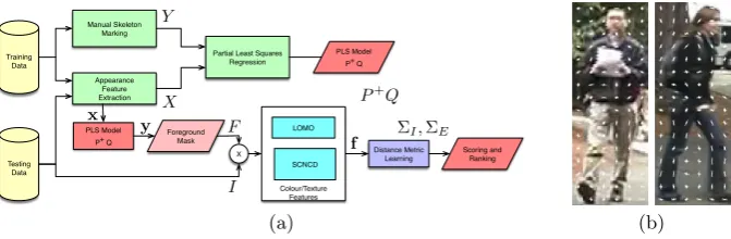
[image:4.459.64.400.51.161.2](a) (b)
Fig. 1. (a) System diagram of the proposed method showing PLS model building, feature extraction and matching; (b) Examples of appearance representation using HOG features.
data sets. In conclusion, we make proposals of how our appearance model might be used for video ReID and perhaps in conjunction with a CNN for data augmentation during network training.
2
Method
In this section, we describe our method which uses a novel skeleton fitting approach to model the image foreground, and then it is combined with robust feature extraction and a distance metric learning to perform matching.
2.1 Partial Least Squares Foreground Appearance Modelling
To predict the skeleton of each person, we learn a regression between the appearance of a person image and a set of landmarks which define a persons skeleton: head, torso and limbs. We use of a Partial Least Squares Regression model to compute the regression. Let X = (x1,x2, ...,xn) be a matrix of image appearances, where each column is
a feature vector extracted from a set of n images. Each vector consists of the con-catenation of several local shape and texture features extracted from different patches of an image. Similarly, Y = (y1,y2, ...,yn) is a matrix where each column consists
of a series of co-ordinates representing skeleton keypoints, one for each corresponding image appearance. In constructingy, each skeleton limb is specified by three points: (p,q,r), representing the ends of the limbs along their centre line and the a point located perpendicular to its axis, defining the limb width.
Partial Least Squares [17] (PLS) is used to find a linear decomposition ofX andY such that:
X=T PT+E, Y =U QT +F, (1)
whereT andU are the score matrices,PandQare the loading matrices, andEandF represent residual matrices ofX andY respectively. Unlike PCA, the PLS algorithm initially computes weight vectors w and c such that greatest variation in X and Y is captured. It can be shown that, in this case, weight vector w is the eigenvector corresponding to the largest eigenvalue ofXTY YTX, and similarly,cis the principal
eigenvector ofYTXXTY. The score vectors are then be used to deflateX andY
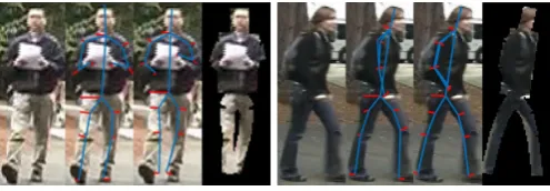
Fig. 2.Examples of PLS skeleton fitting. Each set of four images shows: original, ground-truth, PLS fitted result, foreground segmented mask.
and the process is repeated for X0 and Y0 until the residuals are below a required threshold and all score vectorstanduhave been extracted.
Having calculated the score matrices, T and U, to predict a skeleton given a test instance of an image appearance,xi, then
ˆ
yi=P+Qxi (3)
where P = (TTT)−1TTX0 and Q = (UTU)−1UTY0 and P+ is the Moore-Penrose inverse ofP.
To learn the PLS regression, we take a set of training images and extract HOG features on a regular grid across (Figure 1(b)) the image to form our appearances, and regress them to corresponding landmarks by solving for P+Q. In our method, the appearance X is represented by these Histogram of Oriented Gradients features. Figure 2 shows examples of skeleton fitting on a trained PLS model. The method can be trained to work with both frontal and sideways views.
2.2 Foreground feature extraction and feature weighting
Having located the foreground regions (person) with the PLS skeleton fitting, we apply a feature extraction stage and use weighted Local Maximal Occurrence (LOMO) [10] and Salient Colour Names [21].
Weighted LOMO We modify LOMO [10] such that foreground regions are prioritised over background by feature weighting. LOMO begins by applying a colour normalisa-tion step using the Retinex algorithm [8] to make the images of the same person from different cameras with different illumination conditions appear more consistent. LOMO features are taken from overlapping image patches across the image. HSV histograms and SILTP histograms over three scales [12] are integrated in a combined feature. Then by taking the maximum value in each bin, some invariance to viewpoint variations is gained.
by the percentage of predicted foreground in each feature patch which overlaps with the foreground mask:
fw(B) =
|F∩B|
|B| f(B), (4)
where B is the set of pixels in the image patch and F is the set of pixels labelled foreground. Once all patches in a row have been weighted, the maximum value for each bin in that row can be taken towards the final descriptor. In the experiments presented below, we use the code given by [10] to extract the LOMO features, and alter them as described prior in order to prioritise the features from the foreground.
Salient Colour Names Salient Colour Names [21] define sixteen coordinates in the RGB space of carefully chosen colours, e.g. fuchsia, blue, aqua, lime, etc., extending the Colour Names [19] method, which has only eleven. The RGB colour space is then first quantized into 32×32×32 indexes, d, with each index having 512 quite similar colours, w. The set of colour names are defined as coordinates in the RGB space, Z={z1,z2, ...,z16}, and a mapping (posterior probability) from a given index colour
dand a colour name distribution overZ is calculated. The process is a form of vector quantisation, and similar to the concept of a Bag of Words, and has the advantage for being able to assign multiple similar colours to similar colour name distributions.
Then a mapping posterior probability distribution is factorised into two terms:
p(z|d) = 512 X
j=1
p(z|wj)p(wj|d), (5)
where the first term is a distribution of probabilities p(z|w) calculated as normally distributed variates of the closest K colour name given a quantized colours wj (i.e.
one of those that fall within a discretization bin di). Note that variance of this
dis-tribution is estimated overK−1 coloursnotin the nearest K nearest neighbour set, 1
K−1 P
zk6=zp(zk|zj):
p(z|wj) =
exp(−kz−wjk2/K1−1 P
zi6=zkzi−wjk 2)
P
kexp(−kz−wkk2/K1−1Pzi6=zkzi−wjk
2) (6)
The second term of Eq. 5,p(w|d), models the variancewj at sampledi, against its
mean value,µ, capturing how likely many similar colours are being captured at this position. The more similar colours that are present, the larger this value.
p(wj|d) =
exp(−α|wj−µ|2)
P512
k=1exp(−α|wk−µ|2)
. (7)
Together the two terms capturing how similar or salient colour names are, to the sample colour indexesdi. Multiple similar colours result in similar colour name distributions
Finally, similarly to the LOMO feature, a log transform is applied to the Salient Colour Names features, and each histogram is normalised to a unit length. This de-scriptor is concatenated with the weighted LOMO features to form our final feature descriptor.
2.3 Distance Metric Learning
A metric for measuring the distance between feature descriptors is used at the matching stage. KISSME [6] calculates the distance between two feature vectors as:
τM2(fi,fj) = (fi−fj)T(ΣI−1−ΣE−1)(fi−fj). (8)
with the intra-personal, ΣI, and extra-personal, ΣE, scatter matrices. Here, we use
Cross-view Quadratic Discriminant Analysis (XQDA) [10], which extends KISSME. With KISSME, it is possible to perform dimensionality reduction prior to estimatingΣI
andΣEby performing PCA on the input vectors. XQDA however considers the metric
learning and the dimensionality reduction together. IfDis the original dimensionality of the data andRthe required reduced dimensionality, XQDA learns a subspaceW = (w1,w2, ...,wR)∈RR, whilst simultaneously learning a distance function:
dw(fi,fj) = (fi−fj)TW(Σ
0−1
I −Σ
0−1
E )WT(fi−fj) (9)
where ΣI0 = WTΣ
IW and similarlyΣ
0
E = WTΣEW. Directly optimising dw is not
possible because of the presence of two inverse matrices. As the distribution of intra-personal and extra-intra-personal distances have zero mean, a traditional LDA cannot be used to determineW. Instead, for any projection directionw, which is a column ofW, it is possible to maximise the ratio of variancesσ2
E(w)/σ2I(w). Since however, σE2(w) =
wTΣ
Ew and similarly σ2I(w) = wTΣEw, the objective function is the Generalised
Rayleigh Quotient:
J(w) =w
TΣ Ew
wTΣ Iw
. (10)
We can solve forwby a generalised eigenvalue decomposition in the same way as LDA is solved by maximising
max
w w
TΣ
Ew, s.t.wTΣIw= 1. (11)
The columns of W are the R eigenvectors of ΣI−1ΣE taken in decreasing order of
eigenvalue. Liao et al. [10], have advice on how to make the distance learning calculation robust and computationally efficient. Features extracted from training images using the ground-truth skeletons can be passed to XQDA in order to learn a distance metric.
3
Results and Discussion
– VIPeR: VIPeR [4] contains 632 image pairs, each with a size of 128×48 pixels. Images in the VIPeR data set are captured using two cameras, and have large variations with pose and illumination, and also contain occlusion.
– QMUL GRID: QMUL GRID [13–15] consists of 250 person image pairs, taken from eight disjoint cameras in an underground public transport station. In addition, there are also 775 identities consisting of only one image. Images come in varying sizes. This data set suffers from severe occlusion, as well as variations in pose and illumination. Colour is not as vibrant as in the other data sets, and significant noise is present in the images.
– CUHK03: CUHK03 [9] is the largest widely-used data set in this area, consisting of 1360 identities across two cameras per identity. Each individual has an average of about five images per camera view. Images are obtained by taking stills from a video sequence over several months, and thus suffer from varying illumination conditions. This data set also suffers from pose variations and occlusion. Images are cropped using both manual cropping and a person detector.
From all data sets, we extract Histogram of Oriented Gradients (HOG) features from the standard, non-Retinex images, using a cell size of 6 pixels and a block size of 2 pixels. From the VIPeR data set, we extract the HOG features from the V channel of the HSV colour space, in order to build PLS regression models. The VIPeR data set provides person orientation information for each image, and thus we can split the images in to two partitions - perpendicular to the camera or otherwise. We build separate PLS models for each partition and learn a classifier for model selection. Examples of skeleton fits and the best and worst fitting results on VIPeR are shown in Figure 3. The fitting fails on the few images where a person has their arms raised above their heads.
[image:8.459.132.332.373.472.2](a) (b) (c)
Fig. 3. Examples of the ground-truth and predicted skeletons from VIPeR: (a) A random image with a RMSE of 3.8 pixels; (b) The image with the minimum RMSE of 1.8 pixels; (c) The image with the maximum RMSE of 16.0 pixels. The average RMSE is 5.2 pixels.
VIPeR QMUL GRID CUHK03 r=1 r=5 r=10 r=20 r=1 r=5 r=10 r=20 r=1 r=5 r=10 r=20 PLSAM(v2) 46.3 75.0 85.6 93.9 26.7 47.9 59.0 68.2 65.2 89.8 95.0 97.9 PLSAM(v1) 42.8 71.9 82.0 91.9 23.9 41.8 51.0 61.4 64.6 89.2 94.9 98.1
Null Space [23] 42.3 71.5 82.9 92.1 - - - - 58.9 85.6 92.5 96.3 MLAPG [11] 40.7 69.9 82.3 92.4 16.6 33.1 41.2 53.0 58.0 87.1 94.7 98.0 DeepList [20] 40.5 69.2 81.0 91.2 - - - - 55.9 86.3 93.7 98.0 LOMO+XQDA [10] 40.3 68.3 80.9 91.1 17.3 36.3 44.8 55.4 54.9 85.3 92.6 97.1
[image:9.459.52.407.49.156.2]FPNN [9] - - - 20.7 50.9 67.0 83.0
Table 1. A comparison of state-of-the-art methods: VIPeR [4] data set with 316 person identities were allocated for training, and 316 for testing; QMUL GRID [13–15] data set with 125 person identities were allocated for training, and 900 for testing, where the testing identities contained 125 image pairs and 775 single images; CUHK03 [9] data set with 1160 person identities were allocated for training, and 100 for testing. For the test set, one image of each identity was taken to form the gallery set. Every probe image in the test set was compared to every gallery image in the test set. PLSAM(v2) is with weighted LOMO and Salient Colour Names features and XQDA; PLSAM(v1) is with weighted LOMO and XQDA.
much more robust person descriptor. When concatenated with Salient Colour Names features (PLSAM(v2)), the results increase further. This is unsurprising, due to how distinct are the clothing colours in the VIPeR data set. Overall, we can see a 4.0% increase when comparing our method to the state-of-the-art. The CMC curve plots are given in Figure 4.
For the QMUL GRID data set, we resize each image to 128 × 48 pixels. PLS models are built from HOG features from the V channel of the HSV colour model. Whilst we use two view PLS models for the VIPeR data set, only a single model is used for the QMUL GRID data set because most people in this data set are facing either towards or away from the camera. Examples of skeleton fits and the best and worst fitting results on QMUL GRID are shown in Figure 5. Again, because of lack of sufficient training examples, the fitting fails on people with raised arms. We use the experimental protocols used in various literature [10] [16]. The training and testing sets are split evenly, with 125 identities used for each. The 775 images which do not belong to an image pair are added to the gallery set and we run our experiment ten times, averaging the scores to produce the final result. Table 1 again shows that both PLSAM(v1) and PLSAM(v2) out-perform other methods. As the cameras are located in a busy station, this data has a high level of occlusion and overlapping people in the background and particularly benefits from foreground modelling, producing more representative person descriptors. The CMC curve is plotted in Figure 4.
1 5 101520 30 40 50 60 70 80 90 100 40 50 60 70 80 90 100 Rank % Score VIPeR PLSAM(v2) PLSAM(v1)
Null Space [23]
MLAPG [11]
LOMO+XQDA [10]
1 5 101520 30 40 50 60 70 80 90 100 0 10 20 30 40 50 60 70 80 90 100 Rank QMUL GRID PLSAM(v2) PLSAM(v1) LOMO+XQDA [10] MLAPG [11]
1 5 101520 30 40 50 60 70 80 90 100 0 10 20 30 40 50 60 70 80 90 100 Rank % Score CUHK03 PLSAM(v2) PLSAM(v1) LOMO+XQDA [10]
Null Space [23]
MLAPG [11]
[image:10.459.64.397.53.321.2]FPNN [9]
Fig. 4.CMC on the VIPeR data set [4], QMUL GRID data set [13–15] and, CUHK03 data sets [9]. All of our CMC curves are single-shot results. Results are reproduced from [10], [22], [9] and [11].
model. Whilst we build a CUHK03-specific model for the orientation prediction, for the skeleton fitting stage, we re-used the VIPeR PLS skeleton appearance models, i.e. we do not perform any separate skeleton appearance model training on this data set. Visually the two data sets are quite similar with regards to the camera viewpoints. Our experimentation protocol follow [10] and [9] by splitting the images into a training set of 1160 identities and a test set of 100 identities. We run our experiments twenty times, and average to produce the final results. The results (Table 1), show PLSAM(v1) gives an improvement in the Rank-1 score by 5.7%. With the addition of Salient Colour Names features, PLASM(v2), the Rank-1 score instead improves by 6.3%. The CMC curve can be seen in Figure 4.
4
Conclusions
(a) (b) (c)
Fig. 5.Examples of the ground-truth and the predicted skeleton from the QMUL GRID data set: (a) A random image with a RMSE of 3.9 pixels; (b) The image with the minimum RMSE of 2.3 pixels; (c) The image with the maximum RMSE of 17.7 pixels. The average RMSE over the entire test is 5.3 pixels.
comparative analysis, using state-of-art feature extraction (LOMO and Salient Colour Names) and XQDA distance metric learning, demonstrate a superior matching accuracy when feature extraction is weighted by our foreground estimation. Experiments on the VIPeR, QMUL GRID and CUHK03 data sets show that the proposed method achieves an improvement when vs. the the LOMO feature of 6.0%, 9.4% and 10.3% respectively in the Rank-1 matching rate. An improvement of 4.0%, 9.4% and 6.3% respectively in the Rank-1 matching rate is observed vs. other state-of-the-art methods.
In the case of CUHK03, we show that the skeleton fitting foreground model learnt on one data set, in this case VIPeR, generalises to a different camera view without the need to retrain. For the orientation in VIPeR, we fitted two separate foreground models: one for frontal views and one for sideways views. The model selection process seems to work well in our experiments, and might be extended to multiple views from a network of cameras.
Our further work is focused on using the skeleton fitting in the context of a deep learning (CNN) architecture [1]. We are working on using the PLS model to train a de-convolution CNN to perform foreground modelling and will compare the performance. The non-linearities inherent in neural network regression models might preclude the need to use multiple linear PLS models for varying viewpoints. We also think the PLS models may prove useful in data augmentation for CNN training where the number of training examples is limited, which might be achieved by synthesising appearance model instances from a PCA of the learnt space of variation, e.g. [24].
References
1. Ahmed, E., Jones, M. and Marks, T.K., 2015. An improved deep learning architecture for person re-identification. In Proc. IEEE Conf. on CVPR (pp. 3908-3916).
2. Farenzena, M., Bazzani, L., Perina, A., Murino, V. and Cristani, M., 2010, June. Person re-identification by symmetry-driven accumulation of local features. In Proc. IEEE Conf. on CVPR (pp. 2360-2367).
3. Forssen, P.E., 2007, June. Maximally stable colour regions for recognition and matching. In Proc. IEEE Conf. on CVPR (pp. 1-8).
5. Jojic, N., Perina, A., Cristani, M., Murino, V. and Frey, B., 2009, June. Stel component analysis: Modeling spatial correlations in image class structure. In IEEE Conf. on CVPR (pp. 2044-2051).
6. K¨ostinger, M., Hirzer, M., Wohlhart, P., Roth, P.M. and Bischof, H., 2012, June. Large scale metric learning from equivalence constraints. In IEEE Conf. on CVPR (pp. 2288-2295). 7. Kviatkovsky, I., Adam, A. and Rivlin, E., 2013. Color invariants for Person Reidentification.
In IEEE Trans. on PAMI, 35(7) (pp.1622-1634).
8. Land, E.H. and McCann, J.J., 1971. Lightness and Retinex theory. JOSA, 61(1) (pp.1-11). 9. Li, W., Zhao, R., Xiao, T. and Wang, X., 2014. Deepreid: Deep filter pairing neural network
for person re-identification. In Proc. IEEE Conf. on CVPR (pp. 152-159).
10. Liao, S., Hu, Y., Zhu, X. and Li, S.Z., 2015. Person re-identification by local maximal occurrence representation and metric learning. In Proc. IEEE Conf. on CVPR (pp. 2197-2206).
11. Liao, S. and Li Stan Z., 2015, December. Efficient PSD Constrained Asymmetric Metric Learning for Person Re-identification. In Proc. IEEE Conf. on ICCV (pp. 3685-3693). 12. Liao, S., Zhao, G., Kellokumpu, V., Pietikainen, M. and Li, S.Z., 2010, June. Modeling
pixel process with scale invariant local patterns for background subtraction in complex scenes. In IEEE Conf. on CVPR (pp. 1301-1306).
13. Liu, C., Gong, S., Loy, C.C. and Lin, X., 2012, October. Person re-identification: What features are important?. In ECCV (pp. 391-401). Springer Berlin Heidelberg.
14. Loy, C.C., Xiang, T. and Gong, S., 2009, June. Multi-camera activity correlation analysis. In Proc. IEEE Conf. on CVPR (pp. 1988-1995).
15. Loy, C.C., Xiang, T. and Gong, S., 2010. Time-delayed correlation analysis for multi-camera activity understanding. In IJCV, 90(1), pp.106-129.
16. Loy, C.C., Liu, C. and Gong, S., 2013, September. Person re-identification by manifold ranking. In Proc. IEEE Conf. on ICIP (pp. 3567-3571).
17. Rosipal, R. and Kr¨amer, N., 2006. Overview and recent advances in partial least squares. In Subspace, latent structure and feature selection (pp. 34-51). Springer Berlin Heidelberg. 18. Russakovsky, O., Lin, Y., Yu, K. and Fei-Fei, L., 2012. Object-centric spatial pooling for
image classification. In Proc. ECCV (pp. 1-15).
19. Van De Weijer, J., Schmid, C., Verbeek, J. and Larlus, D., 2009. Learning color names for real-world applications. In IEEE Trans. on Image Processing, 18(7), (pp. 1512-1523). 20. Wang, J., Wang, Z., Gao, C., Sang, N. and Huang, R., 2017. DeepList: Learning Deep
Fea-tures with Adaptive Listwise Constraint for Person Re-identification. In IEEE Transactions on Circuits and Systems for Video Technology.
21. Yang, Y., Yang, J., Yan, J., Liao, S., Yi, D. and Li, S.Z., 2014, September. Salient color names for person re-identification. In ECCV (pp. 536-551).
22. Zhao, R., Ouyang, W. and Wang, X., 2014. Learning mid-level filters for person re-identification. In Proc. IEEE Conf. on CVPR (pp. 144-151).
23. Zhang, L., Xiang, T. and Gong, S., 2016. Learning a discriminative null space for person re-identification. In Proc. IEEE Conf. on CVPR (pp. 1239-1248).
24. Zhang, Q., Bhalerao, A., Helm, E., and Hutchinson C., 2015. Active shape model un-leashed with multi-scale local appearance. In Proc. IEEE Conf. on ICIP (pp. 4664-4668). 25. Zhao, R., Ouyang, W. and Wang, X., 2017. Person re-identification by saliency learning.
![Table 1. A comparison of state-of-the-art methods: VIPeR [4] data set with 316 personidentities were allocated for training, and 316 for testing; QMUL GRID [13–15] data setwith 125 person identities were allocated for training, and 900 for testing, where t](https://thumb-us.123doks.com/thumbv2/123dok_us/9451921.452391/9.459.52.407.49.156/comparison-personidentities-allocated-training-testing-identities-allocated-training.webp)
![Fig. 4. CMC on the VIPeR data set [4], QMUL GRID data set [13–15] and, CUHK03 datasets [9]](https://thumb-us.123doks.com/thumbv2/123dok_us/9451921.452391/10.459.64.397.53.321/fig-cmc-viper-data-qmul-grid-cuhk-datasets.webp)
