METHODS & TECHNIQUES
Determining forward speed from accelerometer jiggle in aquatic
environments
David E. Cade1,§, Kelly R. Barr*,1, John Calambokidis2, Ari S. Friedlaender3,‡and Jeremy A. Goldbogen1
ABSTRACT
How fast animals move is critical to understanding their energetic requirements, locomotor capacity and foraging performance, yet current methods for measuring speed via animal-attached devices are not universally applicable. Here, we present and evaluate a new method that relates forward speed to the stochastic motion of biologging devices as tag jiggle, the amplitude of the tag vibrations as measured by high sample rate accelerometers, increases exponentially with increasing speed. We successfully tested this method in a flow tank using two types of biologging devices and in situon wild cetaceans spanning∼3 to >20 m in length using two types of suction cup-attached tag and two types of dart-attached tag. This technique provides some advantages over other approaches for determining speed as it is device-orientation independent and relies only on a pressure sensor and a high sample rate accelerometer, sensors that are nearly universal across biologging device types.
KEY WORDS: High sample rate noise, Energetic costs, Flow noise, Tag jiggle, Biologging
INTRODUCTION
The forward speed of an organism is a fundamental link between physiology, energy expenditure and ecology across a wide range of spatial and temporal scales (Tucker, 1970), yet accurately and consistently measuring speed in natural environments has proven difficult. An accurate understanding of speed reflects an animal’s locomotor performance (Domenici, 2001), energetic costs (Claireaux et al., 2006; Clark et al., 2010; Videler, 1993; Watanabe et al., 2011) and behavioral state (Aoki et al., 2012; Goldbogen et al., 2006), and also aids in 3D track reconstructions (Laplanche et al., 2015; Wilson and Wilson, 1988). In terrestrial environments, speed can be measured accurately using georeferencing techniques (e.g. von Hünerbein et al., 2000; Weimerskirch et al., 2002). However, global positioning systems (GPS) do not work underwater; thus, in aquatic environments,
forward speed must be measured using multi-sensor, animal-borne tags (Aoki et al., 2012; Fletcher et al., 1996; Sato et al., 2003; Shepard et al., 2008; Wilson and Achleitner, 1985). While these devices have been successful in various contexts, all exhibit disadvantages including high-drag equipment (Kawatsu et al., 2009), orientation constraints (Chapple et al., 2015), a dependence on water clarity (Shepard et al., 2008), and unknown sensor responses within variable flow regimes (Wilson and Achleitner, 1985).
The most direct way to measure speed in aquatic environments is to measure an animal’s change in depth when horizontal motion is small. If an animal’s forward motion with respect to the horizontal plane is equivalent to its pitch, speed can be calculated from an orientation-corrected depth rate (OCDR) (Miller et al., 2004) as:
OCDR¼DdepthsinðpitchÞ1Dtime1: ð1Þ
However, this metric can only be relied on when pitch is accurately determined and sufficiently steep, so these periods are commonly used to perform in situ calibrations for other speed metrics that can then be used to estimate speed for the duration of the device deployment (e.g. Blackwell et al., 1999; Goldbogen et al., 2006; Miller et al., 2016; Sato et al., 2003). One such method relies on the observation that the amplitude of flow noise recorded by a hydrophone increases exponentially with speed (Finger et al., 1979). In situ flow noise measurements are typically regressed against OCDR at high pitch, and then the calibration curve is applied to the entire time series (e.g. Fletcher et al., 1996; Goldbogen et al., 2006; Simon et al., 2009). This method is limited by errors at high and low speed (Goldbogen et al., 2006), errors associated with imperfect regression relationships, and relies on devices with higher battery and memory requirements than other onboard sensors.
Here, we describe an alternative speed estimation method that relies only on a pressure sensor and high sample rate accelerometers (>40 Hz) which are now commonplace in animal-attached tags. Accelerometers have been deployed on swimming animals from diverse taxa including birds (Noda et al., 2016), cartilaginous fish (Gleiss et al., 2011), bony fish (Wright et al., 2014), cnidarians (Fossette et al., 2015), pinnipeds (Ydesen et al., 2014), and both small (Wisniewska et al., 2016) and large cetaceans (Goldbogen et al., 2006). When moving through a dense medium like water at speeds above∼1 m s−1, an accelerometer will record the continuous
jiggling motion that results from passing through a turbulent flow (Movies 1 and 2). We demonstrate the jiggle method using data from three types of multi-sensor tags deployed on cetaceans and also test the method in a flow tank. Our data suggest that in addition to broader applicability, the jiggle method is robust to tag orientation differences and has smaller regression-associated error than the flow noise method.
Received 21 September 2017; Accepted 26 November 2017
1Department of Biology, Hopkins Marine Station, Stanford University, Pacific Grove,
CA 93950, USA.2Cascadia Research Collective, 218 1/2 W. 4th Avenue, Olympia,
WA 98501, USA.3Marine Mammal Institute, Hatfield Marine Science Center,
Department of Fish and Wildlife, Oregon State University, Newport, OR 97365, USA. *Present address: Center for Tropical Research, Institute for the Environment and Sustainability, Department of Ecology and Evolutionary Biology, University of
California, Los Angeles, Los Angeles, CA 90095, USA.‡Present address: Institute
of Marine Sciences, University of California Santa Cruz, Santa Cruz, CA 95064, USA.
§
Author for correspondence ([email protected])
D.E.C., 0000-0003-3641-1242; J.C., 5028-7172; J.A.G., 0000-0002-4170-7294
Journal
of
Experimental
MATERIALS AND METHODS Jiggle method
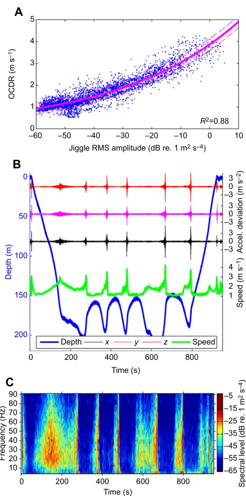
The jiggle method can be implemented using Matlab v2013b or later (www.mathworks.com) code available at https://purl. stanford.edu/gd922zq9141. The method was developed from the observation that the amplitude of stochastic tag motion increases exponentially with increasing speed (Fig. 1), and this tag motion is measured continuously by the device’s accelerometers. Accelerometers measure a combination of both specific (dynamic) and gravity-related (static) acceleration, but speed cannot be determined directly by integrating acceleration as small errors in calibration and tag orientation aggregate when integration of measured quantities is attempted, and because separating the two forms of acceleration is prone to error (Van Hees et al., 2013; Ware et al., 2016). Instead of estimating speed from acceleration, the jiggle method regresses the root-mean-square (RMS) amplitude of accelerometer motion along three axes against speed calculated using OCDR. We then use these regression equations to estimate speed for a given jiggle magnitude across the entire dataset.
The accelerometer jiggle amplitude along each axis is calculated using the function TagJiggle.m by bandpass filtering the magnitude of the high-frequency accelerometer signal using a 128 point symmetric finite impulse response (FIR) filter. A bandpass filter was used for consistency across deployments with up to an 800 Hz sampling rate. However, as most energy in the signal was in the lower frequencies, a high-pass filter could be used for most applications. The most robust filter was determined experimentally. For general use, a 10–90 Hz bandpass filter gives broadly consistent results but the upper limit should be less than the Nyquist frequency (half the sampling rate). The filtered vector is binned (default is ½ second) and centered on each sampling point, and the accelerometer jiggle RMS amplitude (J) of each bin is calculated on a dB scale relative to the accelerometer units.
Like any device that estimates speed based on water movement around an animal, different locations of the device on the animal and the size/shape of the animal itself will lead to different flow conditions and different water velocities at each tag location (Fiore et al., 2017; Schetz and Fuhs, 1999). Thus, calibration in a flow tank is not solely sufficient for speed estimation using any currently existing method, and anin situ calibration must be performed for every deployment. The function SpeedFromRMS.m (available at: https://purl.stanford.edu/gd922zq9141), which can also be used to calculate relationships for other speed metrics (e.g. flow noise), uses OCDR at high pitch angles (default |pitch|>45 deg) as the known speed values, and allows the user to graphically adjust the default parameters to provide greater thresholds for pitch and depth to increase the accuracy of OCDR. The function also allows the user to exclude periods of high roll rate which, for large animals like the baleen whales in this study with a body diameter of 3 m rolling at 40 deg s−1(Segre et al., 2016), could potentially add to the overall
speed experienced by the tag in a non-forward direction. Biologging devices attached with suction cups are periodically subject to sliding on the animal’s body surface, and in the process the tag may adopt a new orientation. To account for this, SpeedFromRMS.m calculates a separate curve for each user-defined period of tag orientation within a deployment. For each section, the script calculates a coefficient of determination (R2) and
produces plots of jiggle RMS amplitude versus OCDR (Fig. 1A) as well as plots of time versus speed calculated from accelerometer jiggle, time versus speed from OCDR, and time versus depth.
When deriving the regression equation, betterR2are obtained by
calculating OCDR across several sample points. Commonly, 1 s
bins are used (e.g. Miller et al., 2016; Sato et al., 2003), but the Matlab scripts allow for flexibility in bin size and the user could choose to match OCDR bin size with jiggle amplitude bin size. Although speed can be calculated from an exponential regression of the accelerometer jiggle along any individual axis or multiple (orthogonal) axes, better results were obtained using a multi-variate, exponential regression across all axes. SpeedFromRMS.m employs the Matlab function fitnlm.m with robust fitting options such that:
R2=0.88
Jiggle RMS amplitude (dB re. 1 m2 s–4)
OCDR (m s
–1
)
–600 –50 –40 –30 –20 –10 0 10
1 2 3 4 5
Depth (m)
0
50
100
150
200
Speed (m s
–1)
Accel. deviation (m s
–2
)
Time (s)
0 200 400 600 800
1 2 3 4 –3 0 3 –3 0 3 –3 0 3
Depth x y z Speed
B
A
Time (s)
Frequency (Hz)
0 200 400 600 800
10 20 30 40 50 60 70 80 90
Spectral level (dB re. 1 m
2 s
–4
)
[image:2.612.317.560.53.541.2]–65 –55 –45 –35 –25 –15 –5
C
Fig. 1. Accelerometer jiggle during a blue whale (bw14_212a) feeding
dive.(A) Jiggle amplitude regressed against periods of orientation-corrected
depth rate (OCDR) when |pitch|>45 deg. (B) Sampling at 250 Hz: the accelerometer signal in all three axes increases in amplitude during descent and ascent and preceding each lunge feeding event. Accelerometer signals are deviations from a 0.4 s running mean of each axis. Speed was smoothed with a 1 s running mean filter. (C) A 250 point fast Fourier transform (FFT) with 25% overlap of they-axis accelerometer signal, calculated and displayed using Triton (Wiggins, 2003).
Journal
of
Experimental
OCDR¼aebðc1Jxþc2Jyþc3JzÞ; ð2Þ
whereaandbare exponential regression coefficients,Jx,JyandJz are the jiggle amplitude of each axis, andc1,c2andc3are restricted
to the range [0 1] and represent the corresponding contributions of each axis to the overall regression equation. For each section of tag orientation, all five coefficients may vary. An R2, the 95%
confidence interval, and 68% and 95% prediction intervals for the resulting regression curve are calculated from standard exponential regression ofJon OCDR, where:
J ¼c1Jxþc2Jyþc3Jz: ð3Þ Finally, the regression equation is applied toJfor all time points such that the resulting speed vector matches the length and sampling frequency of the original data (Figs 1–3).
In vitrotests
Utilizing suction cups designed for deployment on cetacean skin, we attached three types of CATS (Customized Animal Tracking Solutions) video tags (Cade et al., 2016; Goldbogen et al., 2017) with sampling rates of 40, 400 and 800 Hz and an Acousonde (Burgess, 2009) sampling at 400 Hz to the bottom of a recirculating flow tank (Movie 1) with an 18 cm×18 cm cross-sectional area. The devices were exposed to known incrementally increasing flow rates of 0.3 to 3.1 m s−1for periods of 1 min at each speed (Fig. S1). Data
were collected with the tags positioned in four orientations: (A) directly against the flow, (B) directly with the flow, (C) angled against the flow and (D) directly against the flow with only the front two suction cups attached (Fig. S2). The flow tank was controlled with a motor operating at known revolutions per minute (RPM) and the speed at each RPM setting was measured using a Höntzsch flowtherm NT flowmeter (www.hoentzsch.com/en/) at the location where the tag would be placed. The motor generated up to 0.12 m s−1variation in flow speed at each RPM setting, so the
median flow tank speed was regressed against the linearized mean of the corresponding RMS value of the accelerometer jiggle. As the flow tank itself vibrated during the trials (Fig. S1B), the tag was also attached to the outside of the tank and the accelerometer jiggle was calculated at each speed. The amplitudes of the tank vibrations were linearly subtracted from the values recorded in the flow before regressions were calculated (Fig. S2).
The coefficient of determination of the exponential relationships between accelerometer jiggle and flow tank speed (VF) was
calculated for each axis separately and for the overall magnitude of the three accelerometer axes at each of the four tag positions using a single variate version of Eqn 2:
VF¼aebJ: ð4Þ
The correlations were run forJcalculated from the accelerometer jiggle at various frequency ranges (Fig. S3) and this was used to determine both the range and axis that yielded the highest correlation coefficient.
In situtests
The accelerometer jiggle method was tested using data from four tag types deployed on humpback whales (Megaptera novaeangliae Borowski 1781), fin whales [Balaenoptera physalus (Linnaeus, 1758)], blue whales [Balaenoptera musculus(Linnaeus, 1758)] and Risso’s dolphins [Grampus griseus(G. Cuvier 1812)] off the coast of California. All tags were deployed from a 6 m rigid-hull inflatable boat using a 6 m pole under National Marine Fisheries
Service permits 16111, 14534 or 14809 as well as institutional IACUC protocols. Suction cup tags were either CATS video tags or DTAGs (digital sound recording tags) (Johnson et al., 2009) and medium duration dart-attached tags (Szesciorka et al., 2016) were either Acousondes with a custom-modified base or modified TDR-10 tags (Wildlife Computers, Redmond, WA, USA) with an attached accelerometer and additional pressure sensor from CATS (www.cats.is). Accelerometer sampling rates ranged from 40 to 790 Hz. Animal pitch and roll were calculated for DTAG deployments using the DTAG tool kit (https://www.soundtags. org/dtags/dtag-toolbox/) and for CATS and Acousonde deployments using custom-written Matlab scripts (Cade et al., 2016). Accelerometers for DTAGs, Acousondes and CATS deployment mn161117-10 utilized a dynamic range of ±2 g, and remaining CATS deployments recorded at ±4 g.
Accelerometer jiggle amplitudes for 23 baleen whale deployments were calculated and regressed against OCDR at 13 frequency ranges to determine which filtering range consistently gave the best results (Fig. S3). Using the 10–90 Hz frequency range, forward speed was determined with both a univariate and a multivariate regression on OCDR for 27 total deployments on all species. TheR2from a single regression relationship for the whole
deployment was compared with the weighted meanR2 (mR2) of
each tag orientation section. Filtering at 10 Hz removed gravity-related acceleration signals associated with postural changes for our deployments (Sato et al., 2007), but higher frequency floors could also be employed without substantially reducing efficacy (Fig. S3, Movie 2). For deployments with hydroacoustic data (21 of the 27 overall deployments), speed was additionally calculated from the RMS amplitude of flow noise on the hydrophones (Goldbogen et al., 2006; Simon et al., 2009). The acoustic noise in the 66–94 Hz frequency band was calculated from 1 s bins around each data point, and the RMS amplitude was regressed against OCDR using SpeedFromRMS.m. For most varieties of biologging device, an anti-aliasing, pre-digitization high-pass filter is applied to both acoustic and accelerometer data – in the case of acoustics, specifically to reduce flow noise – so care must be taken to choose a frequency band that is not adversely affected by the filtering.
RESULTS AND DISCUSSION
The amplitude of tag jiggle predictably increased with forward speeds greater than ∼1 m s−1 across all tag deployments and tag
types. We confirmed the jiggle–speed relationship in laboratory experiments and we clarified the accelerometer axes and frequency ranges (10–90 Hz) that provided the most robust predictors of speed (Fig. S3, Eqn 2). The lower workable limit of the method was deployment and tag specific with a mean (±s.d.) minimum detected speed of 0.9±0.3 m s−1. At the upper limit, two deep-diving fin
whales with dart-attached Acousondes regularly exceeded 7 m s−1
on steep descents to 300 m with no apparent limitations in the method. In comparison, a flow-noise method used previously in the same species was limited to less than 5 m s−1because of clipping on
the hydrophone (Goldbogen et al., 2006).
We observed a single case of accelerometer clipping that was not associated with the tag breaking the water–air interface (Movie 2). In this case, a humpback whale with a CATS video tag deployed near the animal’s head, the dynamic range of the accelerometer was set to its minimum value. The tri-axial tag jiggle method filtered at 10–90 Hz as described above resulted in an upper detection limit of 6.2 m s−1, but if we used a lower-amplitude 70–90 Hz frequency
band on only they-axis signal (which was perpendicular to gravity
Journal
of
Experimental
for the high-speed event), it reduced the effect of clipping on speed determination (Movie 2). In the Risso’s dolphins, clipping was more common, occurring in two of the four deployments with accelerometers set to ±2 g for a total of 12.9 s out of 20.1 h of tag data. Among all tag deployments and tag types, the jiggle amplitude was correlated with OCDR regardless of whether our analysis included data from individual or multiple accelerometer axes. For most tags, thez-axis accelerometer data slightly improved results, but thez-axis performed poorly in dart-attached tags (Fig. S3). The highest correlations were found using a multi-variate exponential model that included data from all three accelerometer axes (Eqn 2). This method increased mR2by 0.11±0.07 (n=27) over the use of the
vector magnitude of the three axes. Contrary to the tags in the flow tanks, for which including frequencies above 50 Hz did not improve results, R2 values of the correlation for in situ deployments
improved across tag types by including frequencies up to∼90 Hz (Fig. S3). This result implies that while the method can be used with sample rates as low as 40 Hz, sampling at rates higher than 180 Hz will improve speed estimation.
In 16 of 21 deployments where speed was also calculated from flow noise, the jiggle amplitude had a stronger correlation with OCDR, resulting in smaller prediction intervals (95% prediction interval 0.20±0.28 m s−1 smaller), than flow noise. The average
difference between mR2values for the 21 deployments was 0.07±
0.11. Across all 27in situdeployments, mR2for the jiggle method
was 0.82±0.09, while mean mR2 for the flow noise method was
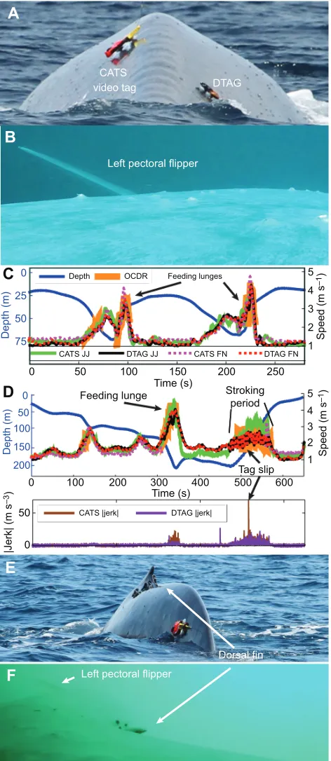
[image:4.612.320.556.61.604.2]0.76±0.16. As a further test and comparison of these methods, we analyzed data from a CATS tag (sampling at 40 Hz) and a DTAG (250 Hz) deployed simultaneously on the same animal (Fig. 2). The four data streams were comparable in both amplitude and inflection for both high- and low-speed events. The CATS tag detached earlier than the DTAG, first sliding back near the flukes. The faster speeds traveled by the peduncle while oscillating were recorded on the CATS tag as a 1 m s−1difference in speed between the two tags
(Fig. 2).
Implications
The method for determining speed from accelerometer jiggle has several notable improvements over previous methods (i.e. flow noise), but some limitations that were common to previous techniques persist. Specifically, our analyses suggest that the jiggle–speed method is: (1) resilient to changes in tag orientation, (2) combines multiple metrics (three accelerometer axes) into a single model (Eqn 2), (3) is less affected by ambient noises than the flow noise method (Fig. 3), (4) has a high theoretical maximum detection limit, (5) is calculated only from low-power sensors that already exist on most devices, (6) is not subject to signal attenuation from pre-digitization high-pass filtering, and (7) exhibits higher model coefficients of determination (compared with flow noise) in all tag deployments sampled higher than 50 Hz. In addition to the ubiquity of accelerometers, the jiggle method has some advantages over propeller-based speed sensors that are commonly analyzed at 1 Hz resolution (Miller et al., 2016; Sato et al., 2003), can stall at both high and low speeds, must be properly oriented in the flow, and, for deployments on animals in highly productive waters or that dive near the sediment, are subject to clogging with particulates.
Because of the potentially high dynamic range of accelerometers, the jiggle method could potentially provide additional and direct validation of the highest swimming speeds in apex predators like sailfish (10 m s−1) (Marras et al., 2015), white sharks (11 m s−1)
(Martin and Hammerschlag, 2012) and pilot whales (9 m s−1)
Left pectoral flipper
CATS
video tag DTAG
A
B
Depth (m)
Time (s)
0 50 100 150 200 250
0
25
50
75 Speed (m s
–1)
1 2 3 4 5
CATS JJ DTAG JJ CATS FN DTAG FN
Depth OCDR
Time (s)
0 100 200 300 400 500 600
0 50 100 150 200
Speed (m s
–1
)
1 2 3 4 5
Depth (m)
CATS |jerk| DTAG |jerk|
|Jerk| (m s
–3
)
50
0
Feeding lunges
Feeding lunge Stroking
period
Tag slip
Dorsal fin
Left pectoral flipper
C
E
F
D
Fig. 2. Speed measurements from deployments of a CATS tag
(bw140806-2) and a DTAG (bw14_218a) on a blue whale.(A) Both tag locations.
(B) Video from CATS tag shows initial tag position near the pectoral flipper. (C) Five metrics of animal speed (JJ, jiggle; FN, flow noise; OCDR, orientation-corrected depth rate when |pitch|>45 deg) smoothed with a 1 s running mean filter showing comparable magnitudes and inflections. (D) The CATS tag slipped to the peduncle. The difference in amplitude of speed measured from the two tags reflects the increased peduncle motion during fluking; at the conclusion of fluking, the two metrics return to comparable values. OCDR during fluking is an unreliable metric of speed because of large oscillations when the travel direction does not coincide with animal pitch. The new position of the CATS tag is shown in E and the perspective from the tag video is shown
in F.
Journal
of
Experimental
(Aguilar Soto et al., 2008). Typical test deployments (e.g. Fig. 1) did not approach the maximum measurable speed. For this example, a jiggle amplitude of 2 g would have correlated with a speed of 9.1 m s−1(17.7 kn), and a full range amplitude of 4 g would have
correlated with a speed of 11.0 m s−1. These values are above the
normal swim speeds of most marine mammals and fish (Block et al., 1992) and within the theoretical range of maximum speeds (10– 15 m s−1) for cavitation-free swimming for lunate-tailed fish and
mammals (Iosilevskii and Weihs, 2008; Svendsen et al., 2016). As clipping was more commonly observed in smaller animals, we recommend increasing accelerometer range to ±4 g for non-baleen whale deployments, though in some systems this may reduce the sensitivity.
The minimum detectable speed for the jiggle method of
∼0.9 m s−1 captures the mean swimming speed of 87% of the
species reviewed by Sato et al. (2007). To detect slower swim speeds using the jiggle method, however, multiple accelerometers with different sensitivities could be used within the same tag. Alternatively, a dedicated device such as a semi-rigid antenna or dome that would vibrate or exhibit omnidirectional displacement in flow could be more sensitive to lower-speed flows. Currently, lower swim speeds are best measured by propeller-based systems (e.g. Sato et al., 2003).
Like any process that relies on models to make predictions outside of the observed data, the jiggle method has error associated with extrapolation from regression. Nevertheless, two tags on the same animal gave nearly identical speeds using the jiggle method (Fig. 2), with a mean difference between tags for data below 20 m of 0.16±0.14 m s−1. Additionally, substantial variance in the
regression is likely due to inaccuracies in the OCDR metric, particularly during active stroking periods when pitch may deviate from the direction of forward travel (e.g. a 45 deg pitch with a 10 deg offset from the actual direction of travel would result in OCDR errors of 19%). When speed was measured in the flow tank, jiggle amplitude was more tightly correlated with speed (meanR2values
were 0.97±0.02 at the frequency range and axis with the highest correlation).
A final implication of the accelerometer–speed relationship is that biologically relevant signals may be obfuscated by high-frequency accelerometer sampling during high-speed events, and caution should be used when analyzing accelerometer signals [e.g. accelerometer jerk (Simon et al., 2012; Ydesen et al., 2014) and acoustic calls (Goldbogen et al., 2014)] that could occur simultaneously with high-speed events. Additionally, animals that do not themselves experience forces above a typical accelerometer sensitivity of ±2 g may nevertheless have datasets with clipped accelerometer readings due to tag jiggle at high speed, and these periods should be scrutinized to ensure that orientation estimation is not affected during these biologically important high-speed events. In conclusion, our analysis provides a greater ability to predict and understand these periods of high-amplitude accelerometer signals that have previously been treated as background noise (Saddler et al., 2017; Stimpert et al., 2015), and details a method for utilizing these signals to estimate animal speed over a considerable range of values.
Acknowledgements
DTAG deployments were conducted as part of the SoCal BRS project led by Brandon Southall and raw tag data were processed by Stacy DeRuiter, Alison Stimpert and Ann Allen. Thanks should also be extended to Elliott Hazen for his feedback on the multi-variate method, to Mark Johnson, Stacy DeRuiter and Alison Stimpert who wrote foundational code on which this method was built, and to two anonymous reviewers who provided helpful feedback.
Depth (m)
Frequency (Hz)
Frequency (Hz)
0
25
50
Time (s)
0 100 200 300 400 500
2 4 –5
0 5
Speed (JJ) Speed (FN)
Feeding lunges
Calls
20 40 60 80
dB re. 1 m
2
s
–4
dB re. 1 m
2
s
–4
Acoustic spectral level 50
100 150
dB
–65 –55 –45 –35 –25 –15 –5
0 10 20 30 40 50 60
200
A
B
0
10
20
Time (s)
0 20 40
1 2 3 –3
0 3
0 20 40 60 80
–65 –55 –45 –35 –25 –15 –5
0 10 20 30 40 50 60
Acoustic spectral level
Speed (JJ) Speed (FN)
0 50 100 150
200 Accelerometer spectral level
dB
Depth (m)
Frequency (Hz)
Frequency (Hz)
i ii iii iv v viviiviiiix x
Accelerometer spectral level
Speed (m s
–1)
Accel. dev. (m s
–2
)
Accel. dev. (m s
–2
)
Speed (m s
–1
[image:5.612.58.295.55.557.2])
Fig. 3. Speed calculated from accelerometer motion and acoustic flow
noise during the presence of other acoustic noise.Acceleration deviation is
thez-axis deviation from a 0.4 s running mean of the accelerometer signal. JJ, jiggle; FN, flow noise. Spectrograms produced using Triton (Wiggins, 2003); dB values are self-referenced in the acoustic spectrograms. (A) A blue whale (bw14_262b) with stereotypical A and B calls (Thompson et al., 1996) recorded on the hydrophone and the accelerometer. Type A calls had most of their acoustic energy in the harmonics that overlapped with the filtered frequencies and showed dramatic increases in flow noise-derived speed. Accelerometer spectrogram is a 250 point FFT with 25% overlap. Acoustic data were downsampled to 8 kHz, and displayed using a 7000 point FFT with 25% overlap. (B) A humpback whale (mn151012-7) with 10 bioacoustic events. Events viii and ix were low-frequency vocalizations common to humpback whales in the NE Pacific (Fournet et al., 2015; Thompson et al., 1986). Event ix was apparent in both the accelerometer and hydrophone signal.
Accelerometer spectrogram used a 200 point FFT with 50% overlap. Acoustic data were recorded at 22.05 kHz and are displayed using an 8192 point FFT
with 25% overlap.
Journal
of
Experimental
Competing interests
The authors declare no competing or financial interests.
Author contributions
Conceptualization: D.E.C., J.A.G.; Methodology: D.E.C.; Software: D.E.C.; Formal analysis: D.E.C.; Investigation: D.E.C., K.R.B., J.A.C., A.S.F.; Writing - original draft: D.E.C., J.A.G.; Writing - review & editing: D.E.C., K.R.B., J.A.C., A.S.F., J.A.G.; Project administration: J.A.G.; Funding acquisition: J.A.C., J.A.G.
Funding
DTAG deployments were funded under grants from the US Navy’s Living Marine Resources Program and the Office of Naval Research Marine Mammal Program. Monterey Bay CATS tag deployments were funded by grants from the American Cetacean Society Monterey and San Francisco Bay chapters, and by the Meyers Trust. Support for D.E.C. was provided by Stanford University’s Anne T. and Robert M. Bass Fellowship and for J.A.G. by the Office of Naval Research’s Young Investigator Award (N00014-16-1-2477) and the National Science Foundation Integrative Organismal Systems award no. 1656691 and the Office of Polar Programs Antarctic Organisms and Ecosystems award no. 1644209.
Data availability
An example data set as well as Matlab scripts for implementation of the method are available at: https://purl.stanford.edu/gd922zq9141.
Supplementary information
Supplementary information available online at
http://jeb.biologists.org/lookup/doi/10.1242/jeb.170449.supplemental
References
Aguilar Soto, N., Johnson, M. P., Madsen, P. T., Dıaz, F., Doḿ ı́nguez, I., Brito,
A. and Tyack, P.(2008). Cheetahs of the deep sea: deep foraging sprints in
short-finned pilot whales off Tenerife (Canary Islands). J. Anim. Ecol. 77, 936-947.
Aoki, K., Amano, M., Mori, K., Kourogi, A., Kubodera, T. and Miyazaki, N.(2012).
Active hunting by deep-diving sperm whales: 3D dive profiles and maneuvers during bursts of speed.Mar. Ecol. Prog. Ser.444, 289-301.
Blackwell, S. B., Haverl, C. A., Boeuf, B. J. and Costa, D. P.(1999). A method for
calibrating swim-speed recorders.Mar. Mamm. Sci.15, 894-905.
Block, B. A., Booth, D. and Carey, F. G.(1992). Direct measurement of swimming
speeds and depth of blue marlin.J. Exp. Biol.166, 267-284.
Burgess, W. C. (2009). The Acousonde: a miniature autonomous wideband
recorder.J. Acoust. Soc. Am.125, 2588-2588.
Cade, D. E., Friedlaender, A. S., Calambokidis, J. and Goldbogen, J. A.(2016).
Kinematic diversity in rorqual whale feeding mechanisms. Curr. Biol. 26, 2617-2624.
Chapple, T. K., Gleiss, A. C., Jewell, O. J. D., Wikelski, M. and Block, B. A.
(2015). Tracking sharks without teeth: a non-invasive rigid tag attachment for large predatory sharks.Anim. Biotelemetry3, 14.
Claireaux, G., Couturier, C. and Groison, A.-L.(2006). Effect of temperature on
maximum swimming speed and cost of transport in juvenile European sea bass (Dicentrarchus labrax).J. Exp. Biol.209, 3420-3428.
Clark, T. D., Sandblom, E., Hinch, S. G., Patterson, D. A., Frappell, P. B. and
Farrell, A. P.(2010). Simultaneous biologging of heart rate and acceleration, and
their relationships with energy expenditure in free-swimming sockeye salmon (Oncorhynchus nerka).J. Comp. Physiol. B180, 673-684.
Domenici, P.(2001). The scaling of locomotor performance in predator–prey
encounters: from fish to killer whales.Comp. Biochem. Physiol. A Mol. Integr. Physiol.131, 169-182.
Finger, R. A., Abbagnaro, L. A. and Bauer, B. B.(1979). Measurements of
low-velocity flow noise on pressure and pressure gradient hydrophones.J. Acoust. Soc. Am.65, 1407-1412.
Fiore, G., Anderson, E., Garborg, C. S., Murray, M., Johnson, M., Moore, M. J.,
Howle, L. and Shorter, K. A.(2017). From the track to the ocean: using flow
control to improve marine bio-logging tags for cetaceans. PLoS ONE 12, e0170962.
Fletcher, S., Le Boeuf, B. J., Costa, D. P., Tyack, P. L. and Blackwell, S. B.
(1996). Onboard acoustic recording from diving northern elephant seals.
J. Acoust. Soc. Am.100, 2531-2539.
Fossette, S., Gleiss, A. C., Chalumeau, J., Bastian, T., Armstrong, C. D.,
Vandenabeele, S., Karpytchev, M. and Hays, G. C. (2015).
Current-oriented swimming by jellyfish and its role in bloom maintenance.Curr. Biol.25, 342-347.
Fournet, M. E., Szabo, A. and Mellinger, D. K.(2015). Repertoire and classification
of non-song calls in Southeast Alaskan humpback whales (Megaptera
novaeangliae).J. Acoust. Soc. Am.137, 1-10.
Gleiss, A. C., Wilson, R. P. and Shepard, E. L. C.(2011). Making overall dynamic
body acceleration work: on the theory of acceleration as a proxy for energy expenditure.Methods Ecol. Evol.2, 23-33.
Goldbogen, J. A., Calambokidis, J., Shadwick, R. E., Oleson, E. M., McDonald,
M. A. and Hildebrand, J. A.(2006). Kinematics of foraging dives and
lunge-feeding in fin whales.J. Exp. Biol.209, 1231-1244.
Goldbogen, J. A., Stimpert, A. K., DeRuiter, S. L., Calambokidis, J., Friedlaender, A. S., Schorr, G. S., Moretti, D. J., Tyack, P. L. and Southall,
B. L.(2014). Using accelerometers to determine the calling behavior of tagged
baleen whales.J. Exp. Biol.217, 2449-2455.
Goldbogen, J. A., Cade, D. E., Boersma, A. T., Calambokidis, J.,
Kahane-Rapport, S. R., Segre, P. S., Stimpert, A. K. and Friedlaender, A. S.(2017).
Using digital tags with integrated video and inertial sensors to study moving morphology and associated function in large aquatic vertebrates.Anat. Rec.300, 1935-1941.
Iosilevskii, G. and Weihs, D.(2008). Speed limits on swimming of fishes and
cetaceans.J. R. Soc. Interface5, 329-338.
Johnson, M., de Soto, N. A. and Madsen, P. T.(2009). Studying the behaviour and
sensory ecology of marine mammals using acoustic recording tags: a review.Mar. Ecol. Prog. Ser.395, 55-73.
Kawatsu, S., Sato, K., Watanabe, Y., Hyodo, S., Breves, J. P., Fox, B. K., Grau,
E. G. and Miyazaki, N.(2009). A new method to calibrate attachment angles of
data loggers in swimming sharks.EURASIP J. Adv. Signal Process. 2010, 732586.
Laplanche, C., Marques, T. A. and Thomas, L.(2015). Tracking marine mammals
in 3D using electronic tag data.Methods Ecol. Evol.6, 987-996.
Marras, S., Noda, T., Steffensen, J. F., Svendsen, M. B. S., Krause, J., Wilson, A. D. M., Kurvers, R. H. J. M., Herbert-Read, J., Boswell, K. M. and Domenici, P. (2015). Not so fast: swimming behavior of sailfish during predator–prey interactions using high-speed video and accelerometry.Integr. Comp. Biol.55, 719-727.
Martin, R. A. and Hammerschlag, N.(2012). Marine predator–prey contests:
ambush and speed versus vigilance and agility.Mar. Biol. Res.8, 90-94.
Miller, P. J. O., Johnson, M. P., Tyack, P. L. and Terray, E. A.(2004). Swimming
gaits, passive drag and buoyancy of diving sperm whales Physeter
macrocephalus.J. Exp. Biol.207, 1953-1967.
Miller, P., Narazaki, T., Isojunno, S., Aoki, K., Smout, S. and Sato, K.(2016).
Body density and diving gas volume of the northern bottlenose whale (Hyperoodon ampullatus).J. Exp. Biol.219, 2458-2468.
Noda, T., Kikuchi, D. M., Takahashi, A., Mitamura, H. and Arai, N.(2016).
Pitching stability of diving seabirds during underwater locomotion: a comparison among alcids and a penguin.Anim. Biotelemetry4, 10.
Saddler, M. R., Bocconcelli, A., Hickmott, L. S., Chiang, G., Landea-Briones, R.,
Bahamonde, P. A., Howes, G., Segre, P. S. and Sayigh, L. S. (2017).
Characterizing Chilean blue whale vocalizations with DTAGs: a test of using tag accelerometers for caller identification.J. Exp. Biol.220, 4119-4129.
Sato, K., Mitani, Y., Cameron, M. F., Siniff, D. B. and Naito, Y.(2003). Factors
affecting stroking patterns and body angle in diving Weddell seals under natural conditions.J. Exp. Biol.206, 1461-1470.
Sato, K., Watanuki, Y., Takahashi, A., Miller, P. J. O., Tanaka, H., Kawabe, R.,
Ponganis, P. J., Handrich, Y., Akamatsu, T., Watanabe, Y. et al.(2007). Stroke
frequency, but not swimming speed, is related to body size in free-ranging seabirds, pinnipeds and cetaceans.Proc. R. Soc. B274, 471-477.
Schetz, J. A. and Fuhs, A. E.(1999).Fundamentals of Fluid Mechanics. Hoboken,
NJ, USA: John Wiley & Sons.
Segre, P. S., Cade, D. E., Fish, F. E., Potvin, J., Allen, A. N., Calambokidis, J.,
Friedlaender, A. S. and Goldbogen, J. A.(2016). Hydrodynamic properties of fin
whale flippers predict maximum rolling performance.J. Exp. Biol.219, 3315-3320.
Shepard, E. L. C., Wilson, R. P., Liebsch, N., Quintana, F., Laich, A. G. and
Lucke, K.(2008). Flexible paddle sheds new light on speed: a novel method for
the remote measurement of swim speed in aquatic animals.Endanger. Species Res.4, 157-164.
Simon, M., Johnson, M., Tyack, P. and Madsen, P. T.(2009). Behaviour and
kinematics of continuous ram filtration in bowhead whales (Balaena mysticetus).
Proc. R. Soc. B Biol. Sci.276, 3819-3828.
Simon, M., Johnson, M. and Madsen, P. T.(2012). Keeping momentum with a
mouthful of water: behavior and kinematics of humpback whale lunge feeding.
J. Exp. Biol.215, 3786-3798.
Stimpert, A. K., DeRuiter, S. L., Falcone, E. A., Joseph, J., Douglas, A. B., Moretti, D. J., Friedlaender, A. S., Calambokidis, J., Gailey, G. and Tyack,
P. L.(2015). Sound production and associated behavior of tagged fin whales
(Balaenoptera physalus) in the Southern California Bight.Anim. Biotelemetry3, 1.
Svendsen, M. B. S., Domenici, P., Marras, S., Krause, J., Boswell, K. M., Rodriguez-Pinto, I., Wilson, A. D. M., Kurvers, R. H. J. M., Viblanc, P. E. and
Finger, J. S.(2016). Maximum swimming speeds of sailfish and three other large
marine predatory fish species based on muscle contraction time and stride length: a myth revisited.Biol. Open5, 1415-1419.
Szesciorka, A. R., Calambokidis, J. and Harvey, J. T. (2016). Testing tag
attachments to increase the attachment duration of archival tags on baleen
whales.Anim. Biotelemetry4, 18.
Journal
of
Experimental
Thompson, P. O., Cummings, W. C. and Ha, S. J.(1986). Sounds, source levels, and associated behavior of humpback whales, Southeast Alaska.J. Acoust. Soc. Am.80, 735-740.
Thompson, P. O., Findley, L. T., Vidal, O. and Cummings, W. C. (1996).
Underwater sounds of blue whales, Balaenoptera musculus, in the Gulf of California, Mexico.Mar. Mamm. Sci.12, 288-293.
Tucker, V. A.(1970). Energetic cost of locomotion in animals.Comp. Biochem.
Physiol.34, 841-846.
Van Hees, V. T., Gorzelniak, L., León, E. C. D., Eder, M., Pias, M., Taherian, S.,
Ekelund, U., Renström, F., Franks, P. W., Horsch, A. et al.(2013). Separating
movement and gravity components in an acceleration signal and implications for the assessment of human daily physical activity.PLoS ONE8, e61691.
Videler, J. J.(1993).Fish Swimming. Dordrecht: Springer Science & Business
Media.
von Hünerbein, K., Hamann, H.-J., Rüter, E. and Wiltschko, W.(2000). A
GPS-based system for recording the flight paths of birds.Naturwissenschaften87, 278-279.
Ware, C., Trites, A. W., Rosen, D. A. S. and Potvin, J. (2016). Averaged
Propulsive Body Acceleration (APBA) can be calculated from biologging tags that incorporate gyroscopes and accelerometers to estimate swimming speed, hydrodynamic drag and energy expenditure for steller sea lions.PLoS ONE11, e0157326.
Watanabe, Y. Y., Sato, K., Watanuki, Y., Takahashi, A., Mitani, Y., Amano, M.,
Aoki, K., Narazaki, T., Iwata, T., Minamikawa, S. et al.(2011). Scaling of swim
speed in breath-hold divers.J. Anim. Ecol.80, 57-68.
Weimerskirch, H., Bonadonna, F., Bailleul, F., Mabille, G., Dell’Omo, G. and Lipp,
H.-P.(2002). GPS tracking of foraging albatrosses.Science295, 1259-1259.
Wiggins, S.(2003). Autonomous acoustic recording packages (ARPs) for long-term
monitoring of whale sounds.Mar. Technol. Soc. J.37, 13-22.
Wilson, R. P. and Achleitner, K.(1985). A distance meter for large swimming
marine animals.South African J. Mar. Sci.3, 191-195.
Wilson, R. and Wilson, M.-P. (1988). Dead reckoning: a new technique for
determining penguim movements at sea.Meeresforschung32, 155-158.
Wisniewska, D. M., Johnson, M., Teilmann, J., Rojano-Doñate, L., Shearer, J.,
Sveegaard, S., Miller, L. A., Siebert, U. and Madsen, P. T.(2016). Ultra-high
foraging rates of harbor porpoises make them vulnerable to anthropogenic disturbance.Curr. Biol.26, 1441-1446.
Wright, S., Metcalfe, J. D., Hetherington, S. and Wilson, R.(2014). Estimating
activity-specific energy expenditure in a teleost fish, using accelerometer loggers.
Mar. Ecol. Prog. Ser.496, 19-32.
Ydesen, K. S., Wisniewska, D. M., Hansen, J. D., Beedholm, K., Johnson, M.
and Madsen, P. T.(2014). What a jerk: prey engulfment revealed by high-rate,
super-cranial accelerometry on a harbour seal (Phoca vitulina).J. Exp. Biol.217, 2239-2243.