Accepted Manuscript
Using hierarchical centering to facilitate a reversible jump MCMC algorithm for random effects models
C.S. Oedekoven, R. King, S.T. Buckland, M.L. Mackenzie, K.O. Evans, L.W. Burger Jr.
PII: S0167-9473(15)00318-7
DOI: http://dx.doi.org/10.1016/j.csda.2015.12.010
Reference: COMSTA 6198
To appear in: Computational Statistics and Data Analysis Received date: 20 March 2015
Revised date: 6 December 2015 Accepted date: 17 December 2015
Please cite this article as: Oedekoven, C.S., King, R., Buckland, S.T., Mackenzie, M.L., Evans, K.O., Burger Jr., L.W., Using hierarchical centering to facilitate a reversible jump MCMC algorithm for random effects models.Computational Statistics and Data Analysis(2015), http://dx.doi.org/10.1016/j.csda.2015.12.010
Using hierarchical centering to facilitate a reversible jump MCMC
algorithm for random effects models
C. S. Oedekovena,∗, R. Kingb, S. T. Bucklanda, M. L. Mackenziea,
K. O. Evanscand L. W. Burger, Jr.c
aCentre for Research into Ecological and Environmental Modelling, School of Mathematics and Statistics, University of St Andrews,
The Observatory, Buchanan Gardens, St Andrews, KY16 9LZ, UK Tel.: +44 1334 461826 Fax: +44 1334 461 800 bSchool of Mathematics, University of Edinburgh,
James Clerk Maxwell Building, The King’s Buildings, Peter Guthrie Tait Road, Edinburgh, UK, EH9 3FD cDepartment of Wildlife, Fisheries & Aquaculture,
Mississippi State University, Box 9690, Mississippi State, MS 39762, USA
*email: [email protected]
Abstract
Hierarchical centering has been described as a reparameterisation method applicable to random effects models. It has been shown to improve mixing of models in the context of Markov chain
Monte Carlo (MCMC) methods. A hierarchical centering approach is proposed for reversible jump MCMC (RJMCMC) chains which builds upon the hierarchical centering methods for MCMC
chains and uses them to reparameterize models in an RJMCMC algorithm. Although these meth-ods may be applicable to models with other error distributions, the case is described for a log-linear
Poisson model where the expected valueλincludes fixed effect covariates and a random effect for
which normality is assumed with a zero-mean and unknown standard deviation. For the proposed
RJMCMC algorithm including hierarchical centering, the models are reparameterized by mod-elling the mean of the random effect coefficients as a function of the intercept of theλmodel and
one or more of the available fixed effect covariates depending on the model. The method is appro-priate when fixed-effect covariates are constant within random effect groups. This has an effect on
the dynamics of the RJMCMC algorithm and improves model mixing. The methods are applied to a case study of point transects of indigo buntings where, without hierarchical centering, the
RJM-1The data and R code for the case study are provided in the annexes of the electronic version of this manuscript. 2* [email protected]
3* http://creem2.st-andrews.ac.uk/
4* http://coedekoven.wix.com/cornelia-oedekoven
*Manuscript
CMC algorithm had poor mixing and the estimated posterior distribution depended on the starting model. With hierarchical centering on the other hand, the chain moved freely over model and
pa-rameter space. These results are confirmed with a simulation study. Hence, the proposed methods should be considered as a regular strategy for implementing models with random effects in
RJM-CMC algorithms; they facilitate convergence of these algorithms and help avoid false inference on model parameters.
Keywords: combined likelihood, “Metropolis Hastings”, point transect sampling, random effects, reparameterisation.
1. Introduction
1
For Bayesian analyses, for a given model, the posterior distribution of the parameters is formed
2
by combining the likelihood of the data with the prior distributions of the parameters. A Markov
3
chain Monte Carlo (MCMC) algorithm is often used to sample from this posterior distribution
4
to obtain inference on the parameters of interest. In the presence of model uncertainty, the
pos-5
terior distribution can be extended to be defined jointly over both parameter and model space.
6
This posterior distribution is often explored using the reversible jump Markov chain Monte Carlo
7
(RJMCMC) algorithm (Green, 1995). However, the art of setting up an RJMCMC algorithm can
8
be challenging on multiple levels. The objective is generally to construct a chain that moves freely
9
between models, efficiently exploring model and parameter space simultaneously.
10
The RJMCMC algorithm entails iteratively updating the parameters conditional on the model
11
(i.e. within-model move) and then updating the model (and corresponding model parameters)
con-12
ditional on the current parameters (i.e. between-model move). Mixing problems for the
within-13
model moves are often due to high autocorrelation within the constructed Markov chain.
Improve-14
ments for mixing within a given model have been investigated in the framework of MCMC with
15
the aim of reducing posterior correlations and increasing the effective sample size by
reparame-16
terisation. In this context, Browne (2004) and Browne et al. (2009) have shown that hierarchical
17
centering (first described by Gelfand, Sahu, and Carlin, 1995) can significantly reduce the
autocor-18
relation within the MCMC algorithm. The use of hierarchical centering in the presence of random
19
effects refers to exchanging the zero-mean of the random effect component, typically assumed to
20
be of normal form, with a model consisting of an intercept and one or more fixed effect covariates.
This will be described in detail in section 2. Papaspiliopoulos, Roberts, and Sk¨old (2007)
investi-22
gated the circumstances when hierarchical centering performs well in comparison to noncentering
23
for MCMC algorithms.
24
Other methods for improving mixing of an MCMC algorithm include parameter expansion,
25
which refers to augmenting the model with additional parameters to form an expanded model
26
(Browne, 2004). The original model is embedded in the expanded one and parameters from the
27
original model can be constructed with parameters from the expanded model. Vines, Gilks, and
28
Wild (1995) describe a method of reparameterisation for random effects models calledsweeping 29
which is suitable also for models with multiple sets of random effects in a generalized linear mixed
30
model (glmm) framework. The idea consists of adding the mean of the random effect coefficients
31
to the intercept of the fixed effects while subtracting the same quantity from each random effect
32
coefficient.
33
For the between-model move in an RJMCMC algorithm (the RJ step), the current model is
34
updated by proposing to move to an alternative model (with given parameters) and accepting this
35
move with some probability. Mixing problems for these between-model moves may arise for
mul-36
tiple reasons, e.g. due to difficulties in finding proposal distributions and updating procedures that
37
produce suitable acceptance probabilities. Besides careful pilot-tuning of proposal distributions,
38
several methods for improving the acceptance rate for the reversible jump step have been proposed.
39
For example, Green and Mira (2001) proposed delayed rejection, where after initial rejection a
sec-40
ond attempt to jump is made with samples generated from a new distribution that may depend on
41
the rejected proposal. Brooks, Giudici, and Roberts (2003) assumed a family for the proposal
dis-42
tribution, where the proposal parameters are chosen to maximize (in some form) the acceptance
43
probability. Al-Awadhi, Hurn, and Jennison (2004) demonstrated that increasing acceptance
prob-44
abilities may be achieved by using a secondary Markov chain with a fixed number of steps that
45
serves to move the value of an RJMCMC proposal closer to a mode before calculating the
accep-46
tance probability for the proposed move. Papathomas, Dellaportas, and Vasdekis (2011) proposed
47
that model mixing for generalized linear models may be improved by using proposal densities that
48
draw samples from parameter subspaces of competing models. Forster, Gill, and Overstall (2012)
49
used the Laplace approximation to integrate out the random effects and orthogonal projections of
50
the current linear predictor onto the proposed linear predictor to produce effective proposals for
glmms.
52
While these previous approaches describe strategies to improve the acceptance rate for RJ steps
53
in general, they can be quite complex to implement. We propose an approach using hierarchical
54
centering that is relatively straightforward to implement for random/mixed effect models. A
par-55
ticular problem that one may encounter with random effect models is that the random effect
coeffi-56
cients may begin absorbing the effect of one or more fixed effect covariates if these are not present
57
in the model at times during the Markov chain. The inclusion of such effects into the model may
58
then be unlikely as they are already accounted for within the random effects. We will demonstrate
59
below that using hierarchical centering provides a simple way of reparameterising the model that
60
will prevent this problem and improve the between-model mixing.
61
Hierarchical centering was initially described by Gelfand, Sahu, and Carlin (1995) as a method
62
to improve convergence for mixed models using MCMC methods. Here we extend the ideas to
im-63
prove mixing in an RJMCMC algorithm. Although our methods may be applicable to models with
64
other error distributions, we consider the case for a log-linear Poisson model with fixed effects and
65
a normally distributed random effect, where the overall likelihood combines the Poisson likelihood
66
for each observation and the normal density for each random effect coefficient. We demonstrate
67
how the Poisson likelihoods and the normal densities are affected differently during a proposal to
68
add a covariate for a regular RJMCMC algorithm and one including hierarchical centering.
69
We demonstrate the improved model mixing using a case study of point transects of indigo
70
buntings (Passerina cyanea L.). Point transects are a form of distance sampling (Buckland et al.,
71
2001) where, in addition to the number of detections during the counts, distance from the point to
72
each detection is collected. This allows estimation of the average detection probabilities at the point
73
and adjustment of counts for imperfect detection. To study the effect of establishing conservation
74
buffers along margins of agricultural fields on density of several species of conservation interest,
75
pairs of points were set up at the edge of fields in a number of states in the USA. These pairs of
76
points consisted of one point on a treatment field and one on a nearby control field without a buffer
77
and these pairs will be referred to as sites in the following. Counts were repeated 1–4 times in
78
each year 2006–2007. We use a combined likelihood including the likelihoods for the detection
79
function and the log-linear Poisson model where counts are adjusted for imperfect detection within
80
the search area around the point (Oedekoven et al., 2014). A random effect for site is included in
the Poisson model to accommodate correlated counts between different sites.
82
In the following we describe how to implement hierarchical centering for RJMCMC, describe
83
the effects on the dynamics of the algorithm, and present updating methods for the RJ step using
84
hierarchical centering (section 2). We then apply the methods to our case study (section 3) and
85
confirm our results with a simulation study (section 4) and discuss our findings (section 5).
86
2. Hierarchical Centering
87
The hierarchical centering described in this paper refers to mixed effect models where a normal
88
distribution is assumed for the random effect. Other distributions may be assumed for the random
89
effect (e.g. Kom´arek and Lesaffre, 2008) to which these methods can be applied but we focus
90
on the normal distribution for simplicity. We describe the case for a glmm with a Poisson error
91
structure, suitable e.g. for fitting a model to correlated count data from repeated measurements.
92
In the following we denote the different groups for the random effect with subscript j and the
93
repeated measurements within the individual groups with subscript r. Here, the expected value
94
λjris modelled via a log-link function with a common intercept,β0and random effect coefficients 95
bj for groups j are included for which normality is assumed. For a mixed effect model without 96
hierarchical centering, the random effect is incorporated into the model under the assumption of a
97
global zero-mean and unknown standard deviation,σb, i.e.bj ∼ N(0, σb2)(e.g. Bates, 2009). Let 98
us assume we have a set ofKcovariates for k= 1, ..., K,xk(and associated coefficients,βk) that 99
can be incorporated as fixed effects. The expected value for the full model including all covariates
100
may then be expressed as:
101
λjr= exp β0+ K X
k=1
xkjrβk+bj !
, bj ∼N µj = 0, σ2b
, (1)
where the xkjr are the measured covariate values corresponding to the rth observation of the re-102
sponse of groupj. While all potential models include the intercept and the random effect, different
103
models included in the RJMCMC algorithm correspond to the combinations of covariates present
104
in the model (i.e. non-zeroβk values). During a between-model move (the RJ step) of an RJM-105
CMC algorithm using this scenario, the proposal to delete or add one (or more) of the covariates
106
(see Appendix A for details on the RJ step).
108
Let us now assume that one covariate, sayx1, was measured at the group level, i.e. values for 109
all repeated measurements for this covariate within a given group were the same, which allows
110
us to use x1 for hierarchical centering. In hierarchical centering, the mean of the random effect 111
is modelled using a combination of the interceptβ0 and one or more covariates that are “pulled 112
from” theλjrmodel from (1) (Gelfand et al., 1995). In the case that the intercept and covariatex1 113
are used for centering, the full model from (1) becomes:
114
λjr = exp K X
k=2
xkjrβk+bj !
, bj ∼N µj =β0+x1jβ1, σb2
. (2)
Note that we omitted the subscript r for covariate x1 in (2) since we assume that the measured 115
values for this covariate were the same for all observations in group j. The proposal to delete
116
or add x1 from the model during the RJ step of the RJMCMC algorithm involves altering the 117
distribution for bj, while the proposal to delete or add any other covariates remains the same as 118
before in (1) (altering the formula forλjr). 119
In the case that allkcovariates were measured at the group level, all covariates may be included
120
in the centering and the full model from (1) becomes:
121
λjr = exp (bj), bj ∼N
µj =β0+ K P k=1
xkjβk, σb2
. (3)
Again, we omitted the subscriptrfor the covariates in the model forµj in (3). In (3), it could be 122
omitted fromλjras well, as there are no covariates in theλjrmodel (or theµjmodel) that may vary 123
between different observations within the same group. However, we keep it for simplicity in the
124
following equations. In this scenario, the formula forλjrremains unchanged during the proposals 125
to delete or add any of the covariates, while the distribution forbj changes for each proposed model 126
move.
127
We note that it is essential that only those covariates are included in the centering (i.e. x1 in 128
(2) or xk withk=1,...,K in (3)) that have the same measured value for all observations within a 129
group (Browne et al., 2009). We refer to a group in terms of the grouping unit for the random
130
effect where grouping should occur to account for intra-group dependence (Davison, 2003). All
observations belonging to the same groupj are modelled with the same random effect coefficient
132
bj in the equations above. 133
The proposed hierarchical centering is only applicable if for at least one covariate, measured
134
values for the respective covariate are the same within a group. If, for example, the grouping unit
135
for a study issite, then the covariate state (the geographical governed entity) can be included in
136
the centering as each site only belongs to one state and all repeated observations for a site belong
137
to the same state. Conversely,Julian daycould not be included as values will likely vary between
138
repeated measurements. As long as this condition holds, any combination of covariates may be
139
included.
140
Hierarchical centering relies on the fact that the random effect coefficients pick up the effect of
141
the covariates included in the centering (given that they have an effect) as they are updated during
142
the within-model move of each iteration of the RJMCMC. Running separate MCMC algorithms
143
(without between-model moves) on the full models from (1), (2) or (3) should result in nearly
144
identical summary statistics for the covariates if the chain was run long enough (since all Markov
145
chains have the same stationary distribution), although mixing might be different for these different
146
parameterisations. However, when including the between-model moves in an RJMCMC algorithm,
147
mixing problems can become more severe, potentially leading to different summary statistics - due
148
to lack of convergence - and hence potentially to the wrong conclusions. Here, convergence and,
149
hence, obtaining correct results may depend on which scenario and initial starting values were
150
used. If, e.g. under the scenario of (1), the random effect coefficients absorb the effect of covariate
151
x1, the chain may get “stuck” in models that do not include x1. For the scenarios of (2) and 152
(3), moves to models including covariate x1 would be favoured if the random effect coefficients 153
absorbed the effect of x1 as then the coefficients will be closer to their modelled means. We will 154
show below that this is due to the fact that here different parts of the likelihood are affected by a
155
proposed model move compared to (1).
156
2.1. Effects of hierarchical centering on RJMCMC dynamics 157
Using either one of the models forλjr from above ((1), (2), or (3)), the likelihood of the log-158
(modified from McCulloch and Searle, 2001):
160
Ln(β, σb) = J Y j=1 Rj Y r=1
(λjr)njrexp (−λjr)
njr! ×
1 q
2πσ2 j
exp
−(bj −µj) 2 2σ2
j
, (4)
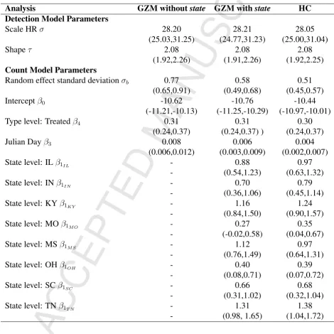
where vector β contains the coefficients for covariates included in the models and njr are the 161
observed measurements of the response. The indicesj = 1,2,3, ..., J represent the groups for the
162
random effect andr= 1,2,3, ..., Rjindices for the different measurements taken for thejth group. 163
Hence for each group of observations, j, the probability of observing njr under the log-linear 164
Poisson model with expected value ofλjris multiplied for all observations within that group, which 165
is then multiplied by the normal density of the random effect coefficientbj. The only coefficients 166
that influence both parts of this likelihood, i.e. the Poisson likelihood for the observations and the
167
normal densities, are the random effect coefficients, regardless of which scenario is used from the
168
previous section.
169
Consider now, that we use this likelihood as part of calculating the acceptance probabilities for
170
updating the model as well as the fixed and random effect coefficients in an RJMCMC algorithm
171
(e.g. Oedekoven et al., 2014). Both the Poisson likelihood and the normal densities are higher if
172
the observed value of the response or the random effect coefficients are closer to their respective
173
means (λjrorµj, respectively). Hence, combining what we know from (1) - (4), it is evident that 174
the Poisson likelihoods will improve if the variation that is not accounted for by the fixed effect
175
coefficients is picked up by the random effect coefficients (which – as well as the fixed effect
176
coefficients of the current model – are updated during the within-model move). On the other hand,
177
the normal densities will return higher values for random effect coefficients close to their mean
178
values.
179
Intuitively, one may think that a problem arises for a between-model move (using models from
180
(1)) when a covariate, sayx1, may have an effect but is not included in the current model. Then, 181
the random effect coefficients may begin to absorb this effect and in this manner, adjust the value
182
for λjr to improve the likelihood. This may result in a “tug-of-war” between the Poisson likeli-183
hood trying to adjust the coefficients in such a manner that the effect ofx1 is accounted for and, 184
on the other hand, the normal densities trying to keep the coefficients close to their mean, i.e. zero
185
for (1)). This will typically also result in an inflated random effect standard deviation since the
random effect coefficients are replacing some unexplained variability attributable to x1. If this 187
has indeed occurred, an acceptance ofx1 into the model during a between-model move proposal 188
may become very unlikely as its effect is already accounted for by the random effect coefficients.
189
Hence, during a proposal to addx1, the new model withx1 will create inferiorλjr. These will then 190
return decreased likelihood values even if the randomly drawn value(s) for x1 would produce a 191
larger likelihood under circumstances before the effect has been absorbed by the random effect
co-192
efficients. In other words, the values of the random effect coefficients are dependent on the model.
193
A strategy to account for this could be to jointly update the coefficient value(s) for covariate x1 194
and the values for the random effect coefficients. However, this complicates the RJ step involving
195
more complex proposal distributions.
196
Alternatively, this issue may be addressed using hierarchical centering since proposing to add
197
x1 using either (2) or (3) into the model will not changeλjr (and the Poisson likelihood). Here, 198
the random effect coefficients absorb the effects of the covariates included in the model (given
199
they have an effect) within the mean of the random effect distribution (in addition to the intercept
200
β0). Using (2) this would be only covariate x1; using (3) this would be covariates xk with k = 201
1,2,3..., K. The only part of the likelihood that is affected when updating this/these covariate(s)
202
for within-model and between-model moves are the normal densities from (4). It is likely that, on
203
average, the normal densities improve for the individual random effect coefficients as these will
204
on average be closer to their assumed mean. Asλjrremains the same, likelihood values returned 205
by the Poisson part of (4) remain the same (which also increases the speed of calculating the
206
acceptance probability for the RJ step since only the normal densities need to be evaluated).
207
2.2. RJ updating methods using hierarchical centering 208
To demonstrate how to implement hierarchical centering, we use a simple example where
209
during the between-model move of iteration t + 1 we propose to include covariate x1 into an 210
intercept-only model, say model m. Suppose that at iteration t the current state of the chain is
211
model m, where λjr = exp (bj) with bj ∼ N(µj =β0, σ2b) from (3) (although if x1 is the only 212
covariate available,K = 1and (2) and (3) are equivalent). During iteration t+ 1 we propose to 213
move to model m0 by adding covariate x1. Hence, modelm0 is defined as λ0jr = exp b0j
with
214
b0
j ∼ N µ0j =β00 +x1jβ10, σ0b
2. For simplicity, let us assume that covariate
egorical covariate with only two levels where the first level is absorbed in the intercept β00 and
216
the second level has an associated coefficient β0
1; hence,x1 is either 0 for the first level or 1 for 217
the second level. We note that these methods also apply in the case that the covariate used for
218
centering has more than two factor levels. Let us further assume that all measurements within a
219
groupj belong to the same level ofx1 and that, for simplicity, we have 200 groups where groups 220
j = 1, ...,100belong to the first level ofx1 and groupsj = 101, ..,200belong to the second level 221
ofx1. We use the identity function as the bijective function (King et al., 2010): 222
u00 =β0, β00 =u0, β10 =u1 (5)
and draw samplesufrom the respective proposal distributions for the parametersβ00 andβ10. See
223
Appendix A for further details.
224
In the following, we describe two different ways for implementing the RJ step. The difference
225
between them lies in the definition of the proposal distributions for the new parameters for the
226
between-model move, and, hence, should only have an influence on the acceptance probability
227
of this move. The second approach (Section 2.2.2) uses more information compared to the first
228
(Section 2.2.1) and should, on average, return higher acceptance rates for this move. Either method
229
should not have an influence on estimated posterior summary statistics of the parameters in the final
230
model given that the chain had an adequate burn-in.
231
2.2.1. Hierarchical centering using predefined proposal distributions 232
For this method, we define proposal distributions for the coefficients β0, β00 and β10. If, for 233
example, normal proposal distributions are used, we define the proposal distributions for
coeffi-234
cientsβ0
1 asβ10 ∼ N µ01, σ10
2, for some predefined
µ0
1 andσ10. Equivalently, the normal proposal 235
distributions for the interceptsβ0 andβ00 are defined asβ0 ∼ N(µ0, σ02)and β00 ∼ N µ00, σ00 2 236
(for some predefinedµ0,σ0,µ00 andσ00). 237
2.2.2. Hierarchical centering using updated proposal distributions 238
Here, the mean µ0 of the proposal distribution for the global interceptβ0 of modelmand the 239
meansµ0
0andµ01of the proposal distributions for the coefficientsβ00 andβ10 of modelm0are updated 240
t+ 1, we take the overall mean¯bt
j of the current values of all random effect coefficientsbtj (i.e. 242
β0t+1 ∼N(µt+10 = ¯bt
j, σ02)including groupsj = 1, ...,200). To update theµ01 at iterationt+ 1, we 243
take the mean¯b0t
j of the random effect coefficients from iterationtbelonging to the second level of 244
covariatex1. Hence, we haveβ10t+1 ∼N(µ01t+1 = ¯b0jt, σ102)only including groupsj = 101, ...,200. 245
To updateµ00 at iterationt+ 1, we take the mean¯b0tj of all random effect coefficients belonging to
246
the first level of covariatex1 (i.e. groupsj = 1, ...,100). 247
3. Case study: point transects of indigo buntings
248
3.1. The data 249
To establish the success of planting herbaceous buffers around agricultural fields in several
250
South-eastern and Midwestern US states, point transect surveys were conducted from a large
num-251
ber of randomly selected fields during the breeding season (May−July) of 2006−2007 in each
252
participating state (Fig. Appendix B, Oedekoven et al., 2013). Survey points on control fields
253
of the same agricultural use and located within 1−3km were surveyed concurrently. Each pair
254
of adjacent points from a treated and control field was considered a site. Points were located at
255
the edge of the fields. Observers recorded all male indigo buntings (all singles) detected either
256
visually or aurally during a 10-minute count at each point in one of five predetermined distance
257
intervals (0−25, 25−50, 50−100, 100−250, 250−500 and >500m). It is assumed that indigo
258
buntings distribute themselves evenly within and in the various possible habitats adjacent to the
259
field. Only those sites that were surveyed at least once in each survey year were included in the
260
analysis. These 446 sites were located in nine states: Georgia, Iowa, Illinois, Kentucky, Missouri,
261
Mississippi, Ohio, South Carolina and Tennessee.
262
3.2. Methods 263
As the models from (1) to (3) assume perfect detection on the plot, we needed to supplement
264
these with a model to adjust counts for imperfect detection. We used the methods described in
265
Oedekoven et al. (2014): a detection function was fitted to the frequency of detections in each
266
distance bin. This detection function was used to estimate the effective area,ν (the area beyond
267
which as many birds were seen as were missed within, Fig. Appendix B), which was incorporated
268
into the log-linear Poisson model for the counts as an offset (Buckland et al., 2001). The full model
consisted of the likelihood component for the detection function and the likelihood component for
270
the counts (see Oedekoven et al., 2014 for details). In addition, we extended the count model to
271
include a subscriptpto denote the two points at each site. With the offset included, the full model
272
without hierarchical centering from (1) became:
273
λjpr = exp β0+x01jβ1+ K X
k=2
xkjprβk+bj + ln (ν) !
, bj ∼N µj = 0, σ2b
. (6)
Site was used as the grouping factor for the random effect. Available covariates werestate(x1, a 274
factor with nine levels),year(x2, factor with two levels: 2006 and 2007, corresponding tox2 = 0 275
andx2 = 1, respectively),Julian day(x3, discrete with observed integers ranging from 142 to 211) 276
andtype(x4, factor with two levels: control (x4 = 1) or treatment (x4 = 1) plot). Factor covariate 277
stateis represented by a vectorx1j of length8either with eight entries zero for observations from
278
state Georgia – as the coefficient of the baseline state is absorbed in the intercept – or with seven
279
entries zero, and one1, indicating which state site j was in, and β1 is a column vector of eight 280
coefficients. Note that similar to (2) we omitted the subscripts randpfor covariate x1 since the 281
values for this covariate were the same for all observations in group j. Furthermore, we did not
282
include a subscript for the effective areaν as, for simplicity, we only considered global detection
283
functions, i.e. without stratification or covariates in the detection model. Hence, given a model
284
and parameter value(s) for the detection function, estimates of the effective areaν were the same
285
for all counts. Asstatewas the only covariate with consistent values for all measurements within
286
a given site, we were limited to using only one covariate within the hierarchical centering (i.e.
287
corresponding to (2)). With hierarchical centering using the state covariate, x1, the full model 288
from (2) became:
289
λjpr = exp K X
k=2
xkjprβk+bj + ln (ν) !
, bj ∼N µj =β0+x01jβ1, σ
2 b
. (7)
To estimate parameters of both the detection function (θ) and the count model (β, σb) in one step, 290
we combined the likelihood components pertaining to the respective models using the combined
291
likelihood, Ln,y(β, σb,θ) = LyG(θ)Ln(β, σb|θ)described by Oedekoven et al. (2014). In com-292
effective area as an offset in (6) or (7). The data contained J = 446 sites. Rj, the maximum 294
number of visits to a site, ranged from 2 to 8 between sites as each site was visited 1-4 times in
295
each of the two survey years. As each site contained two points, we extended (4) accordingly:
296
297
Ln(β, σb|θ) = 446 Y j=1 2 Y p=1 Rj Y r=1
(λjpr)njprexp (−λjpr)
njpr! ×
1 q
2πσ2 j
exp
−(bj −µj) 2 2σ2
j
. (8)
As distances were recorded in intervals (rather than exact distances), the likelihood for the detection
298
function component, LyG(θ) was defined as the multinomial likelihood wherefi represents the 299
probability that a detected animal is in theith distance interval (for details on calculating the fis 300
see Appendix B):
301
LyG(θ) = n! I Q i=1
ni! I Y i=1
fni
i . (9)
Here,nrepresents the total number of detected animals and ni the number of animals detected in 302
theith distance interval. As detection probabilities generally dropped below 0.1 beyond 100m, we
303
limited the analysis to the three innermost distance intervals (0–25, 25–50, 50–100m).
304
For the detection models, we considered the half-normal and hazard-rate key functions as the
305
two (non-nested) model options (Buckland et al., 2001). For the count model, we considered
306
all possible combinations of the covariatesyear, type, Julian dayandstate. We ran two different
307
analyses on the same data. For the first analysis we used “regular” RJMCMC methods with a global
308
zero-mean random effect (as shown in (6)) which we refer to as the global zero-mean analysis
309
(GZM).
310
For the second analysis we implemented hierarchical centering by pulling the interceptβ0 and 311
covariate statefrom the λjpr model and included them in the model for the random effect mean 312
(as shown in (7)). This analysis will be referred to as HC in the following. We used predefined
313
proposal distributions for all parameters. These were the same for both analyses (see Table B.1).
314
Prior model probabilities were equal and the identity function similar to (5) used for the
bijec-315
tive function of any proposed move. For both analyses, we placed the same set of uniform priors
316
on the parameters (Table B.1).
317
For each analysis, the chain was started from the most parsimonious models: the half-normal
detection function and a count model containing the fixed effect intercept and a random effect for
319
site. We ran 200 000 iterations for each analysis, the first 20 000 were considered as the burn-in
320
phase. The effective sample size was calculated for each parameter in the preferred model using
321
the functioneffectiveSizefrom the R packagecoda. We express it as the effective sample size per
322
1000 iterations that the chain was in the preferred model to make this quantity comparable between
323
the results of different methods.
324
3.3. Results 325
The preferred detection model was the hazard-rate function with posterior probability of 1.00
326
for both analyses (Table B.2). Estimated probabilities for the count models differed between the
327
methods. For GZM, the preferred count model included the covariates typeand Julian daywith
328
probability 0.85. The alternative model included the additional covariateyear and was selected
329
during the remaining 15% of the iterations. The covariate state was never included in any of
330
the models for this method. By contrast, all models included statefor HC. The preferred model
331
includedtype,Julian dayandstate(0.95 probability) and the second most preferred model included
332
type,Julian day,yearandstate(0.05 probability).
333
While the probabilities of being in the model were similar for the covariates year, Julian day 334
andtypebetween the two analyses, the probability of statebeing in the model was 0.00 for GZM
335
and 1.00 for HC. To investigate further, we used a range of different initial starting values and
336
models to assess convergence. In particular, when we initialised the chain so that state was in
337
the initial model for the GZM analysis, the posterior probability for state was 1.00. Repeated
338
simulations provided the same output with state not being updated in GZM. Hence, for GZM
339
the resulting model probabilities were conditional on the model that the chain was started with.
340
In contrast, consistent results were obtained for the HC analysis, irrespective of initial values or
341
initial model choice of the Markov chain.
342
Summary statistics for the parameters resulting from both GZM analyses (started with and
343
without state) and the HC analysis are given in Table B.3. Means and 95% credible intervals
344
(CRI) were nearly identical between all methods for the parameters of the hazard-rate detection
345
function. Means and 95% CRIs were also similar for the count model parameters between the three
346
varied, CRIs overlapped between all three methods. The exception was the random effect standard
348
deviation of the count model which was very different for GZM started without statecompared
349
to the other two analyses. The mean was larger for GZM withoutstate and CRIs did not overlap
350
those of the other two methods. This was likely due to the random effects coefficients absorbing
351
thestateeffect.
352
We refrain from including the GZM withoutstateanalysis in the comparison of effective
sam-353
ple sizes as here, due to non-convergence, the posterior distribution differed from the other two
354
analyses (GZM withstateand HC). The effective sample sizes for detection function parameters
355
were similar between all the GZM withstateand HC analyses (Table B.4). Effective sample sizes
356
for count model parameters were generally smaller for HC compared to GZM with stateexcept
357
for the random effect standard deviation and the intercept. It was notable that the effective sample
358
sizes for thestatecoefficients were consistently at least two times but up to over 12 times larger for
359
GZM with statecompared to HC. The only notable increase in effective sample size from GZM
360
withstateto HC was for the random effects standard deviation with 2.46 for GZM withstateand
361
8.54 for HC.
362
4. Simulation study
363
The following simulation study was used to investigate whether our proposed methods would
364
consistently improve model mixing. In particular, for a covariate with nested random effects that
365
was part of creating the pattern in the response variable, we investigated whether posterior model
366
probabilities would differ between hierarchical centering and regular RJMCMC methods. Using
367
(2), we simulated 300 data sets of approximately 500 observations each that were similar to our
368
case study. The response variable followed a Poisson distribution for which the expected valueλjr 369
was modelled as a function of a linear term, sayJulian day x2, and random effects coefficients, 370
bj for the jth site. The bj were simulated using a factor covariate with five levels, say state x1 371
(with four associated coefficientsβ1 randomly drawn from a uniform distribution,U(−2.6,0.8), 372
during each simulation and the coefficient of the first level absorbed in the interceptβ0), to model 373
the mean µj of their normal distribution, bj ∼ N µj =β0+x01jβ1, σb2
and the random effects
374
standard deviationσb = 0.7. Sites were nested within states with25−35sites per state and repeat 375
observations (2−6, subscript r) per site. We also created a dummy variable, a factor covariate
with eight levels which was not part of the model for generating the response. Similar tox1, this 377
dummy variable had constant levels within each random effect group. However, the levels of the
378
dummy variable to which random effects groups were attributed were chosen at random and did
379
not match the pattern for attributing random effects groups to levels ofx1. 380
Each data set was analysed using two different approaches equivalent to GZM without state 381
and the HC methods above. The former refers to “regular” RJMCMC methods with a global
zero-382
mean random effect (as shown in (1)). The latter refers to hierarchical centering methods where
383
the interceptβ0, stateand the dummy variable were included in the model for the random effect 384
mean (as shown in (3)).
385
The RJMCMC analyses for each data set were initiated with the models for λjr and µj that 386
only contained the intercept and random effects coefficients between the two models combined
387
and the chains for both analysis methods had the same initial coefficient values. Both approaches
388
used the same proposal distributions for new parameter values, the same mechanism for updating
389
the model, i.e. proposing to add or delete covariates depending on whether it was currently in the
390
model (including the dummy variable), and the same MH algorithm for updating parameter values.
391
Each analysis included 100 000 iterations where the first 10 000 were considered burn-in.
392
For the GZM withoutstateanalysis, posterior probabilities ofstatebeing in the model were 0
393
for all 300 data sets. By contrast, posterior probabilities ofstatebeing in the model for the HC
anal-394
ysis were on average 0.94 (95% CRI ={0.62,1.00}) across all 300 data sets. The random effects
395
standard deviation was generally overestimated for those models withoutstate, i.e. those iterations
396
of the HC analysis wherestate was not in the model (posterior distribution mean 0.92, 95% CRI
397
= {0.69,1.24}) and for all models from the GZM analysis (0.96, {0.71,1.32}). By contrast, for
398
those models with statefrom the HC analysis, the posterior distribution of this parameter (0.66,
399
{0.49,0.88}) was more accurate with a mean closer to the known true value 0.7. The marginal 400
posterior probability that the dummy variable was included in the model was zero for all 300 data
401
sets and both analysis methods.
402
5. Discussion
403
The purpose of incorporating random effects in count models is generally to model variation
404
that is otherwise unaccounted for. When using RJMCMC methods, the danger exists that the
random effect coefficients account for too much of the variation and prevent the inclusion of a
406
fixed effect covariate into the model – a problem that is not limited to the linear predictor for the
407
Poisson distribution. We demonstrated this case with our GZM analysis that was initiated without
408
state in the model. Due to poor mixing (between models) leading to lack of convergence, the
409
covariate state was never selected. This would have led to incorrect inference as the sampled
410
values are not from the posterior distribution due to poor mixing. In addition, for this analysis
411
the resulting random effect standard deviation was much larger compared to the HC analysis of
412
the same data. Both these findings, the poor model mixing and inflated random effects standard
413
deviation for the GZM analysis, were confirmed by our simulation study.
414
For the HC analysis of the case study, the model was also initiated withoutstatebut revealed
415
posterior probabilities ofstatebeing in the model of 1.00. Furthermore, the mean and 95% CRI of
416
the random effects standard deviation were smaller compared to the GZM withoutstateanalysis.
417
Both these findings were again confirmed by our simulation study. For both analyses of the case
418
study that were initiated withoutstatein the model, GZM and HC, the random effect coefficients
419
absorbed the effect of thestatecovariate. For GZM, this prevented the inclusion of this parameter
420
into the model. For HC, this favoured the inclusion ofstateinto the model as here this covariate
421
was part of the model for the random effect mean. Here, the chain was able to explore models with
422
stateas a covariate due to improved mixing between models.
423
Unsurprisingly, implementing hierarchical centering had little effect on the remaining
covari-424
ates in the model as these were not involved in the centering. However, we could not confirm
425
the findings of Browne (2004), that implementing hierarchical centering would improve the
ef-426
fective sample size for the covariate involved in the centering. He compared the effective sample
427
sizes for the same covariate in two different MCMC chains, one with hierarchical centering and
428
one without. For our case study, effective sample sizes for coefficients involved in the centering
429
were mostly larger for GZM withstatecompared to HC except for the intercept and the random
430
effect standard deviation where, using hierarchical centering, the effective sample size increased
431
3.47-fold.
432
Overall we showed that implementing hierarchical centering in the context of RJMCMC
algo-433
rithms improves mixing between models and, hence, improves the inference on model parameters.
434
For our case study, summary statistics for covariates not involved in the centering were nearly
identical between the GZM and the HC analyses. However, inference on thestatecovariate using
436
the GZM analysis could potentially have led us to believe falsely that this covariate had no effect
437
on densities of indigo buntings.
438
Acknowledgements
439
The National CP-33 Monitoring Program was funded by the Multistate Conservation Grant
440
Program (Grant MS M-1-T), which is supported by the Wildlife and Sport Fish Restoration
Pro-441
gram and managed by the Association of Fish and Wildlife Agencies and US Fish and Wildlife
442
Service. Further support was provided by the US Department of Agriculture (USDA) Farm
Ser-443
vice Agency and USDA Natural Resources Conservation Service Conservation Effects Assessment
444
Project. Collaborators included the AR Game and Fish Commission, GA Department of Natural
445
Resources (DNR), IL DNR/Ballard Nature Center, IN DNR, IA DNR, KY Department of Fish and
446
Wildlife Resources/KY Chapter of The Wildlife Society, MS Department of Wildlife, Fisheries
447
and Parks, MO Department of Conservation, NE Game and Parks Commission, NC Wildlife
Re-448
sources Commission, OH DNR, SC DNR, TN Wildlife Resources Agency, TX Parks and Wildlife
449
Department, Southeast Quail Study Group and Southeast Partners In Flight. The first author was
450
supported by a studentship jointly funded by the University of St Andrews and EPSRC, through
451
the National Centre for Statistical Ecology (EPSRC grant EP/C522702/1), with subsequent funding
452
from EPSRC/NERC grant EP/1000917/1. We thank Prof. William Browne, University of Bristol,
453
for inspiring the presented methods and for commenting on a draft manuscript.
454
Appendix A. RJMCMC algorithm
455
In general, the posterior distributionπ(δm, m|x)is given as the distribution encompassing the 456
joint posterior distribution of models and parameters (Green, 1995; King et al., 2010) with:
457
π(δm, m|x)∝L(x|δm, m)p(δm|m)p(m). (A.1)
Here, L(x|δm, m) is the probability density function of the data x conditional on model m with 458
current parameter valuesδm,p(δm|m)is the prior probability for model parametersδmconditional 459
Suppose that we propose to move from modelmwith parametersδmto modelm0 with param-461
etersδ0
m0 during the between-model move (RJ step) of an RJMCMC algorithm. We define uand 462
u0as random samples from some proposal distribution for the respective parameters. To transform
463
parametersδm intoδ0m0 we use a bijective function which may have the form(δm0 , u0) = g(δm, u). 464
Then, the acceptance probability is given bymin(1, A)whereAcan be expressed as:
465
A= π(δ 0
m0, m0|x)P(m|m0)q0(u0)
π(δm, m|x)P(m0|m)q(u)
∂g∂((δδmm, u, u))
. (A.2)
P(m0|m)is the probability of proposing to move to modelm0 given that the chain is in model m, 466
q(u)andq0(u0)are the proposal densities ofuandu0. ∂g(δm,u)
∂(δm,u)
is the Jacobian. 467
For the within-model move (the MH step) of the RJMCMC algorithm we use a random walk
468
single-update Metropolis-Hastings algorithm (Hastings, 1970; Metropolis et al., 1953).
469
470
Appendix B. The detection function component
471
To calculate the offset for (6) and (7), we used the probability density function of observed
472
distances,f(y) = π(y)g(y)/R0wπ(y)g(y)dy, where wis the truncation distance (Buckland et al.,
473
2001). The function describing the distribution of birds is given for points byπ(y) = 2y/w2 and 474
the detection function is given byg(y). We included two detection functions as model options in 475
the RJMCMC algorithm, the half-normal (g(y) = exp (−y2/2σ2)) and the hazard-rate (g(y) = 1− 476
exp (−(y/σ)−τ)). When using interval distance data (as opposed to exact distance measurements), 477
fi is defined as the probability that a detected animal is in the ith interval which is delineated by 478
the cutpointsci−1 andciand is given by: 479
fi = ci
R
ci−1
f(y)dy
w R
0
f(y)dy
, (B.1)
where the truncation distance,wcorresponds to the outermost cutpoint. Thefi feed into the like-480
lihood component given in (9).g(y)is also used to calculate the effective area, which for points is 481
given byν = 2πR0wyg(y)dy.
Literature cited
483
Al-Awadhi, F., Hurn, M., Jennison, C., 2004. Improving the acceptance rate of reversible jump
484
MCMC proposals. Statistics & Probability Letters 69, 189–198.
485
Bates, D., 2009. Computational methods for mixed models. R package version 0.999375-31. Tech.
486
rep., http//lme4.r-forge.r-project.org/.
487
Brooks, S. P., Giudici, P., Roberts, G. O., 2003. Efficient construction of reversible jump Markov
488
chain Monte Carlo proposal distributions. Journal of the Royal Statistical Society B 65(1), 3–55.
489
Browne, W. J., 2004. An illustration of the use of reparameterisation methods for improving
490
MCMC efficiency in crossed random effect models. Multilevel Modelling Newsletter 16, 13–25.
491
Browne, W. J., Steele, F., Golalizadeh, M., Green, M. J., 2009. The use of simple
reparameteriza-492
tions to improve the efficiency of Markov chain Monte Carlo estimation for multilevel models
493
with applications to discrete time survival models. Journal of the Royal Statistical Society A 172
494
(3), 579598.
495
Buckland, S. T., Anderson, D. R., Burnham, K. P., Laake, J. L., Borchers, D. L., Thomas, L., 2001.
496
Introduction to Distance Sampling. Oxford University Press.
497
Davison, A. C., 2003. Statistical Models. Cambridge University Press.
498
Forster, J. J., Gill, R. C., Overstall, A. M., 2012. Reversible jump methods for generalised linear
499
models and generalised linear mixed models. Statistics and Computing 22 (1), 107–120.
500
Gelfand, A. E., Sahu, S. K., Carlin, B. P., 1995. Efficient parametrisations for normal linear mixed
501
models. Biometrika 82 (3), 479–488.
502
Green, P. J., 1995. Reversible Jump Markov chain Monte Carlo computation and Bayesian model
503
determination. Biometrika 82(4), 711–732.
504
Green, P. J., Mira, A., 2001. Delayed rejection in reversible jump Metropolis-Hastings. Biometrika
505
88(4), 1035–1053.
Hastings, W. K., 1970. Monte Carlo sampling methods using Markov Chains and their
applica-507
tions. Biometrika 57(1), 97–109.
508
King, R., Morgan, J., Gimenez, O., Brooks, S., 2010. Bayesian Analysis for Population Ecology.
509
CRC Press.
510
Kom´arek, A., Lesaffre, E., 2008. Generalized linear mixed model with a penalized Gaussian
mix-511
ture as a random effects distribution. Computational Statistics and Data Analysis 52, 3441–3458.
512
McCulloch, E. C., Searle, S. R., 2001. Generalized, Linear, and Mixed Models. John Wiley &
513
Sons, Inc.
514
Metropolis, N., Rosenbluth, A. W., Rosenbluth, M. N., Teller, A. H., Teller, E., 1953. Equations of
515
state calculations by fast computing machines. Journal of Chemical Physics 21, 1087–1091.
516
Oedekoven, C. S., Buckland, S. T., Mackenzie, M. L., Evans, K. O., Burger, L. W., 2013.
Improv-517
ing distance sampling: accounting for covariates and non-independency between sampled sites.
518
Journal of Applied Ecology 50(3), 786–793.
519
Oedekoven, C. S., Buckland, S. T., Mackenzie, M. L., King, R., Evans, K. O., Burger, L. W.,
520
2014. Bayesian methods for hierarchical distance sampling models. Journal of Agricultural,
521
Biological, and Environmental Statistics 19 (2), 219–239.
522
URLhttp://dx.doi.org/10.1007/s13253-014-0167-0
523
Papaspiliopoulos, O., Roberts, G. O., Sk¨old, M., 2007. A general framework for the
parametriza-524
tion of hierarchical models. Statistical Science 22 (1), 5973.
525
Papathomas, M., Dellaportas, P., Vasdekis, V. G. S., 2011. A novel reversible jump algorithm for
526
generalized linear models. Biometrika 98 (1), 231–236.
527
Vines, S. K., Gilks, W. R., Wild, P., 1995. Fitting multiple random effects models. Tech. rep., MRC
528
Biostatistics Unit, Cambridge.
List of Figures
530
B.1 Left: Distribution of surveys conducted as part of the CP-33 Monitoring Program
531
between 2006-20011 (source: http://www.fwrc.msstate.edu/bobwhite/monitoring/index.asp).
532
Right: frequency of detections in the three distance bins (0–25, 25–50, 50–100m)
533
as rescaled blue histogram bars; probability density of observed distances (PDF)
534
using means from the posterior distribution of parameters of the hazard-rate
detec-535
tion function (see Table B.3, black line); the slope of the red line is the slope of
536
the PDF at distance zero;rhois the radius of the effective areaν; the red polygon
537
represents the proportion of birds missed within rho and is equal in size to the
538
green polygon which represents the proportion of birds detected betweenrhoand
539
the truncation distance w of 100m (Buckland et al., 2001). See Appendix B for
540
more details. . . 23
List of Tables
542
B.1 Means and standard deviations (SD) of normal proposal distributions for model
543
parameters as well as lower and upper boundaries for uniform prior distributions
544
for model parameters. HN and HR refer to the half-normal and the hazard-rate
545
detection functions respectively. We note that the random effect standard deviation
546
and the intercept for the count model were always in the model. . . 25
547
B.2 Posterior model probabilities for the analyses of the indigo bunting data. Shown
548
are results from the GZM analysis (global zero-mean for the random effect) and
549
results from the HC (hierarchical centering) analysis. Both analyses were started
550
withoutstatein the initial model. . . 26
551
B.3 Mean and 95% credible intervals for models with highest posterior support from
552
the analyses of the indigo bunting data. Results are from the analyses GZM (global
553
zero-mean) started withoutstate, GZM started withstateand HC (hierarchical
cen-554
tering) started withoutstate. For models withstate, thestatelevel GA is absorbed
555
in the intercept. . . 27
556
B.4 Effective sample sizes per 1000 iterations that the chain was in the respective
pre-557
ferred model for model parameters from the analyses of the indigo bunting data:
558
GZM (global zero-mean) withstatein the initial model and HC (hierarchical
cen-559
tering). . . 28
Table B.1: Means and standard deviations (SD) of normal proposal distributions for model parameters as well as lower and upper boundaries for uniform prior distributions for model parameters. HN and HR refer to the half-normal and the hazard-rate detection functions respectively. We note that the random effect standard deviation and the intercept for the count model were always in the model.
Parameters Mean SD Lower Upper
Detection Function Parameters
Scale HN: 37 2 10 99
Scale HR: 28 2 10 99
Shape HR: 2 1 1 10
Count Model Parameters
Random effect standard deviation – – 0 1
Intercept: – – -20 -7
Year level: 2007 0.05 0.2 -1 1
Type level: Treated 0.3 0.1 0 1
Julian Day: 0.0055 0.003 -0.1 0.1
State level: IL 0.4 0.5 -2.5 2.5
State level: IN 0.3 0.5 -2.5 2.5
State level: KY 0.7 0.5 -2.5 2.5
State level: MO 0 0.5 -2.5 2.5
State level: MS 0.5 0.5 -2.5 2.5
State level: OH 0 0.5 -2.5 2.5
State level: SC 0.2 0.5 -2.5 2.5
Table B.2: Posterior model probabilities for the analyses of the indigo bunting data. Shown are results from the GZM analysis (global zero-mean for the random effect) and results from the HC (hierarchical centering) analysis. Both analyses were started withoutstatein the initial model.
Analysis GZM HC
Detection Model
CDS: Hazard-rate key 1.000 1.000
Count Model
Type + JD 0.851 0.000
Year + Type + JD 0.149 0.000
Type + JD + State – 0.946
Table B.3: Mean and 95% credible intervals for models with highest posterior support from the analyses of the indigo bunting data. Results are from the analyses GZM (global zero-mean) started withoutstate, GZM started withstate and HC (hierarchical centering) started withoutstate. For models withstate, thestatelevel GA is absorbed in the intercept.
Analysis GZM withoutstate GZM withstate HC
Detection Model Parameters
Scale HRσ 28.20 28.21 28.05
(25.03,31.25) (24.77,31.23) (25.00,31.04)
Shapeτ 2.08 2.08 2.08
(1.92,2.26) (1.91,2.26) (1.92,2.25)
Count Model Parameters
Random effect standard deviationσb 0.77 0.58 0.51
(0.65,0.91) (0.49,0.68) (0.45,0.57)
Interceptβ0 -10.62 -10.76 -10.44
(-11.21,-10.13) (-11.25,-10.29) (-10.97,-10.01)
Type level: Treatedβ4 0.31 0.31 0.30
(0.24,0.37) (0.24,0.37) ) (0.24,0.37)
Julian Dayβ3 0.008 0.006 0.004
(0.006,0.012) (0.003,0.009) (0.002,0.007)
State level: ILβ1IL - 0.88 0.97
- (0.54,1.23) (0.63,1.32)
State level: INβ1IN - 0.70 0.79
- (0.36,1.06) (0.45,1.14)
State level: KYβ1KY - 1.16 1.24
- (0.84,1.50) (0.90,1.57)
State level: MOβ1M O - 0.27 0.35
- (-0.02,0.58) (0.04,0.67)
State level: MSβ1M S - 1.12 0.97
- (0.76,1.49) (0.64,1.31)
State level: OHβ1OH - 0.40 0.39
- (0.08,0.71) (0.07,0.72)
State level: SCβ1SC - 0.66 0.68
- (0.31,1.02) (0.32,1.04)
State level: TNβ1T N - 1.31 1.38
Table B.4: Effective sample sizes per 1000 iterations that the chain was in the respective preferred model for model parameters from the analyses of the indigo bunting data: GZM (global zero-mean) withstatein the initial model and HC (hierarchical centering).
Parameter GZM withstate HC
Detection Model
Scale HR 5.04 4.99
Shape 6.18 5.92
Count Model
Random effect standard deviation 2.46 8.54
Intercept 0.57 1.06
Type Treatment 71.15 64.07
Julian Day 0.58 0.26
State IL 4.15 0.64
State IN 3.63 0.69
State KY 2.58 0.42
State MO 3.38 0.28
State MS 3.30 0.57
State OH 3.54 0.39
State SC 4.41 0.69
We consider a hierarchical centering approach for reversible jump MCMC algorithms.
We describe the case for a log-linear Poisson model with mixed effects.
The zero-mean of the random effect is replaced with part of the linear predictor.
We apply the methods to point transect data of indigo buntings and simulated data.
Our methods improve model mixing and inference on parameters.