doi:10.4236/iim.2010.211073 Published Online November 2010 (http://www.SciRP.org/journal/iim)
Nonsmooth Optimization Algorithms in Some Problems of
Fracture Dynamics
V. V. Zozulya
Centro de Investigacion Cientifica de Yucatan A.C, Colonia Chuburná de Hidalgo, Yucatán, México
E-mail: [email protected]
Received October 16, 2009; revised July 10, 2010; accepted September 15, 2010
Abstract
Mathematical statement of elastodynamic contact problem for cracked body with considering unilateral re-strictions and friction of the crack faces is done in classical and weak forms. Different variational formula-tions of unilateral contact problems with friction based on boundary variational principle are considered. Nonsmooth optimization algorithms of Udzawa’s type for solution of unilateral contact problem with friction have been developed. Convergence of the proposed algorithms has been studied numerically.
Keywords: Unilateral Contact, Friction, Crack, Variational Principles, Boundary Variational Functional, Nonsmooth Optimization Algorithm
1. Introduction
The mathematical formulation of the elastodynamic problem for a cracked body, that takes into account the possibility of crack edge contact interaction and the for-mation of areas with close contact, adhesion and sliding, was presented first in [1]. The algorithm for the solution of this problem was elaborated in [2] and is based on a theory of subdifferentional functionals and the finding of their saddle points. Many examples of the crack faces contact interaction and friction influence on the fracture mechanics criterions have been considered in the book by Guz and Zozulya [3] and review papers [4-6]. In these cases the contact area is “a priori” unknown and the uni-lateral conditions have to be imposed on the relative dis-placements and the mutual tractions. The unilateral con-tact restriction with friction can be written as an inequal-ity for the displacement and traction vectors. As a result a complete set of boundary conditions at crack faces is written as a system of equations and inequalities. The presence of inequality type boundary conditions implies the boundary problems to be nonlinear, which requires the investigation of corresponding boundary value prob-lems.
Mathematical formulation of the problem of crack faces contact interaction in the dynamic case has bee done in [3-5,7]. Since the constraints concern boundary variables only, it is natural to look for a numerical
solu-tion by means of boundary integral equasolu-tion (BIE) method. Approach is based on use of fundamental solu-tions. In [8] BIE formulation via energy method is based on boundary min-max principle, i.e., a principle ex-pressed in terms of the boundary unknowns. First time boundary variational formulation of elastodynamic con-tact a problem with frication was proposed in [2] and then was extended and applied to elastodynamic prob-lems for bodies with cracks with considering unilateral frictional contact of the crack faces in Guz and Zozulya [3,5].
for-mulation and numerical solution of the unilateral contact problems can found in [17,18].
The aim of this paper is to present variational formula-tion of the elastodynamic problem for body with crack with considering possibility for unilateral crack faces contact interaction with friction. Variational formulation of the problem, which is based boundary variational principle is presented. Nonsmooth functionals that cor-respond to unilareral frictional contact conditions are constructed. The case of the crack in infinite elastic me-dia is considered in more details. In order to study con-vergence of the proposed algorithms, two problems re-lated to the crack faces contact interaction under action of the harmonic tension-compression and shear waves have been solved numerically using BIE method.
2. Classical Formulation of the Problem
Let us consider dynamical loading of crack in an infinite homogeneous, lineally elastic body. The crack is des- cribed by a corresponding oriented middle surface since we suppose that only small deformations occur. We assume that displacements of body points and their gra-dients are small.
In this case in Rn\ (n2, 3)the differential equa-tions of equilibrium in displacement may be presented in the form
2
,
ij j i t i
A u b u x Rn\,
0 1 1
[ , ]
( , ) ( ( , ))
n n
i i k
t t t
q t q
x F x (1)
The operator Aij for an isotropic body has the form
( )
ij ij k k i j
A , (2)
where and are Lame constants, 0 and ,
ij
is a Kronecker’s symbol, i xi denotes the partial derivatives with respect to space, t t
de-notes the partial derivatives with respect to time. Throughout this paper we use the Einstein summation convention.
If the problem is defined on an infinite region, then the solution of Equation (1) is uniquely determined by as-signing displacements and velocity vectors in the initial instant of time. Then the initial conditions are
0 0
´0 0
( , ) ( ) , ( , ) ( ),
i i t i i
u x t u x u xt v x x V (3)
Additional conditions at the infinity must be satisfied
1
( , ) ( )
i
u x t O r , ij( , )x t O r( 2) for r in 3-D case (4)
1
( , ) (ln( ))
i
u x t O r
, ij( , )xt O r( 1) for r
in 2-D case (5)
Here r is the distance in the 3-D and 2-D Euclidian spaces respectively.
The differential operator P uij: j pi is called stress
operator. It transforms the displacements into the trac-tions. For homogeneous isotropic elastic medium it has the forms
ij i k ij n k i
P n n (6)
Here ni are components of the outward unit normal
vector, n ni i is a derivative in direction of the
vec-tor n x( ) normal to the surfaceV.
The contact forces ( , )q xt qi( , )x et i which arise on
the cracks edges during the interaction are denoted by
( , )t ( , )t ( )
q x σ x n x (7)
where σ( , )xt ij( , )x et iej is the strain tensor;
( )ni( ) i
n x x e , ni( )x ni( )x ni( )x ; ni( )x and
( )
i
n x are the normal unit vectors directed to the posi-tive side of the opposite cracks edges.
The displacement discontinuity vector characterizes mutual displacements of the cracks edges
( , ) ( , ) ( , )
i i i
u t u t u t
x x x , (8)
where ui( , )xt and ui( , )xt are displacements of
op-posite cracks edges.
Furthermore, we impose the following Signorini con-straints
, 0 , ( ) 0 ,
n o n n o n
u h q u h q
x (9)
and Coulomb’s friction law:
0 , ,
n t n t t
k q k q
q u q u q
x (10)
with λτ u x( ) q for x ; the Coulomb’s friction coefficient k 0 is here assumed to be con-stant.
Here the normal and tangential components of the dis-placement discontinuity on are denoted by
( , ) ( , ) ( , )
n i i
u x t u x t n x t ,
( , )t ( , )t un( , ) ( )t
u x u x x n x , (11)
and the normal and tangential components of the con-tact forces on are denoted by
( , ) ( , ) ( )
n i i
q xt q x t n x , ( , )t ( , )t qn( , ) ( )t
q x q x x n x . (12)
bound-ary value problem (1)-(5) with considering Signorini contact conditions (9) with friction (10).
In classical elastodynamics the equations of motion (1) and initial conditions (2) must be satisfied exactly (see [19]). This means that the components of the displace-ment vector should be functions of the class
2.2 1.0
(Rn ) ( )
C C . Here Ck l,(Rn )is a func-tional space of functions, with k smooth derivatives with respect to the space coordinates and l smooth deriva-tives with respect to the time. In order to satisfy all the equations of elastodynamics in the classical sense, the components of the stress-strain state should belong to the following functional spaces
2,2 1,0
1,0 0,0
( ) ( ) , ,
( ) , ( )
n
i ij
n ij i
u R
R p
C C
C C (13)
These requirements of classical elastodynamics are very stringent. Therefore many important physics and engineering problems, in particular problems with uni-lateral restrictions and friction, have no classical solution. For this reason it is necessary to consider “weakened” formulations to elastodynamic problems. With such an approach it is not necessary to fulfill all the elastody-namics equations in the classical sense.
3. Variational Formulation of the Problem
without Contact Conditions
In order to formulate an elastostatic contact problem for body with crack in week form we will consider the boundary variational principle introduced in [2,5,11,12].
In [2,5] it have been shown that in the case if body with crack occupied infinite regionthe boundary varia-tional funcvaria-tional may be presented in the form
1 2
( , ) ( , ) ( , ) ( , , ) ( , ) ( , )
B i j ji
i i
u t u t F t dSdt
p t u t dSdt
u p y x x y
y y
(14)
where p x( , )t pi( , )x et i p x0( , )t q x( , )t , p x0( , )t is a vector of given loading applied to the crack edges,
( , )t
q x is a vector of contact forces,.
The boundary variational functional (14) is smooth and Gateaux-differentiable, therefore the following con-dition of functional minima take place
( ) 0
B
u (15)
and the problem of finding minima is equivalent to the following integral equation
( , ) ( , , ) ( , )
j ji i
u t F t dSdt p t
x x y y (16)We can represent boundary variational functional (14) in the form
1 2
( , ) , ,
B
u p F u u p u (17)
where F is matrix integral operator defined in (16). Then variational formulation of an elastodynamic problem for cracked body without unilateral constraints (7) and friction (8) is as follows:
* *
* *
, ( , )
, ( , )
( , ) min { [ , ]} B
B
B B
Find such tha t
u p K u p
u p K u p
u p u p (18)
where
1/ 2,1 1/ 2.0
( , )
{ ( ) , ( ), }
B
K u p
u H p H x (19)
4. Nonsmooth Functionals for Unilateral
Contact Conditions with Friction
In order to formulate boundary conditions in form of inequalities (9) and (10) in week form let us consider a maximal monotone operators i:uipi . For each
maximal monotone operator i may be defined with
accuracy up to a constant component convex semi-con-tinuous from below functional ji such, that i ji.
Here is denoted the subdifferential of the nonsmooth functional (see [18] for details).
4.1. Signorini Boundary Conditions in Functional Space
Let 1/ 2,1
( )
n
u
H and 1/ 2,0
( )
n
q H
satis- fy following conditions un h0, qn0.
0
, ( ) 0
n n
q u h , Here , denotes the duality
pairing between the functional spaces H1/ 2,0( )
and
1/ 2,1
( )
H . Then corresponding functional has the form
0
0 , if ( )
, otherwise
n
n n
u h
u
(20) The conjugate functional has the form
0 , if 0 ( )
, otherwise
n c
n n
q
q
(21)
4.2. Boundary Conditions with Coulomb Friction
Lets 1/ 2,1 2
( ( ))
u H and 1/ 2,0 2
( ( ))
satisfy following conditions if q kqn then u 0,
if q kqn then u q and also
(kqnq ), t u 0. Here , denotes the
duality pairing between the functional spaces
1/ 2,1 2
(H ( )) and (H1/ 2,0( ))2
. Then corre-sponding functional has the form
( ) ,
u q u (22)
The conjugate functional has the form
0 , if ( )
, otherwise
c kqn
q
q (23)
4.3. Signorini Boundary Conditions with Friction
These boundary conditions may be considered as com-bination of the previously considered boundary condi-tions. Really lets un H1/ 2,1( ) and
1/ 2,0
( )
n
q H
satisfy following conditions
0 n
u h
, qn0 , qn, ( un h0) 0 and also
1/ 2,1 2
( ( ))
u H and 1/ 2,0 2
( ( ))
q H
sat-isfy following conditions if q kqn then u 0 ,
if q kqn then t u q and also
(kqnq ) t u 0 . We consider functionals
such that
, ( ) ( ) ( )
n n un
u u and
, ( ) ( ) ( )
c c c
n n qn
q q
(24) These functionals have the form
0 ,
, , if
( ) , otherwise t n n u h q u
u (25)
,
0 , if 0 , ( )
, otherwise
c n n
n
q kq
q
q (26)
4.4. Sets of Admissible Displacements and Traction for Signorini Boundary Conditions with Friction
For variational formulation of the unilateral contact problems with friction also are used sets of admissible displacements
, , ( , ) ( , ) ( ) ( )
B n B n
K u p K u p K u K u ,
, ( , ) ( , ) ( )
B n B n
K u p K u p K u ,
, ( , ) ( , ) ( ) ( )
B B n
K u p K u p K u K u ,
1/ 2,1
0
( ) { ( ) , 0}, , }
n un h t
K u u H x
(27)
1/ 2,1
( ) { ( ) ,
0 for and for , }
t
n t t n
k q k q
K u u H u
q u q q x
and traction
, , ( ) ( ) ( ) ( )
c c
B n T n
K σ K σ K σ K σ ,
, ( ) ( ) ( )
c
B n T n
K σ K σ K σ , , ( ) ( ) ( )
c
B T
K σ K σ K σ
1/ 2,0
( ) { ( ) , 0, }
c
n qn
K σ σ H x (28)
1/ 2,0 ( ) { ( ) , , } c n k p
K σ σ H q x
5. Variational Formulation of the Problem
with Contact and Friction
In order to formulate an elastodynamic contact problem for body with crack in variational form we consider functional (17) on the set of admissible displacements (27) or admissible traction (28).
In the first case the problem is formulated in the form
*
* , ,
* *
( , ) ( , )
( , ) sup inf { ( , )} B n
B
B B
Find and such tha t
u K u p
p K u p
u p
u p u p (29)
In the second case the problem is formulated in the form
* *
, ,
* *
( , ) ( , )
( , ) inf sup { ( , )}
c
B B n
B B
Find and such tha t
u K u p p K u p
u p
u p u p (30)
In order to formulate an elastodynamic contact prob-lem for body with crack in week form using nonsmooth functionals (23) and (24) we will consider the boundary variational principle in the form
* *
* *
, , , ,
, ( , )
( , ) inf sup { ( , )} B
B n B n
Find and such tha t
u p K u p
u p
u p u p
(31)
where
, , ( , ) ( , ) , ( )
B n B n
u p u p u (32)
In the same way we can consider the complementary functional
, , ( , ) ( , ) , ( )
c c
B n B n
u p u p q . (33)
In this case the problem well be
* *
* *
, , , ,
, ( , )
( , ) sup inf { ( , )} B
c c
B n B n
Find and such tha t
u p K u p
u p
u p u p
(34)
sets of restrictions (27) and (28) are complicate, they contains unilateral constraints (9) and (10). Functionals (30) and (31) are more complicate and nonsmooth, but the set of restrictions (19) is simple, it does not contain unilateral constraints (9) and (10). Which for is more is preferable depend on algorithm used for numerical solu-tion of the problem. It is necessary to mensolu-tion that the boundary variational principles are usually used with BEM.
6. Dual Variational Formulation and
Uzawa’s Optimization Algorithm
We can reformulate above variational problems using duality feature. On these dual formulations are based Uzawa’s nonsmooth optimization algorithms. Let us consider dual formulations and corresponding Uzawa’s algorithms for the problems under consideration.
6.1. Bounadry Variational Principles I
Let us introduce functional
* * * *
( , , ) B( , ) , ( )
u p q u p q u
L (35)
which is considered on the following sets of restric-tions
, B( )
u p K u , , ( )
c n
q K σ (36)
Dual to (31) variational formulation of the contact problem with friction for elastic body with crack has the form
* * *
,
* * *
, ( , ) ( )
( , , ) inf sup sup ( , , ) c
B n
u p K u p q K σ
u p q u p q
L L (37)
The Uzawa’s algorithm includes the following steps: 1) specify an initial value 0
, ( ) c n
q K σ ,
2) solve the minimization problem for known qn and determine the unknown quantity u pn, nK u pB( , )
, ( , )
, ( , )
( , , ) inf sup { ( , , )}
inf sup ( , ) , ( ) B
B
n n n n
n
B
u p K u p
u p K u p
u p q u p q
u p q u
L L
(38)
3) correct the quantity qn to satisfy the constraints
,
1
( )[ ( )]
c n
n n n
K σ
q P q u (39)
where
,( ) c n
K σ
P is the operator of projection in
1/ 2,0
( )
H on , ( )
c n
K σ and coefficient is se-lected so as to provide the best convergence of the algo-rithm,
4) proceed to the next step of iteration.
6.2. Bounadry Variational Principles II. Let us Introduce Functional
* * * *
( , , ) B( , ) , c( )
u p u u p u q
L (40)
Which is considered on the following sets of restric-tions
, B( )
u p K u , u Kn,( )u (41)
Dual to (34) variational formulation of the contact problem with friction for elastic body with crack has the form
* * *
,
* * *
, ( , ) ( )
( , , ) inf sup sup ( , , ) c
B n
u p K u p q K σ
u p u u p u
L L (42)
The Uzawa’s algorithm includes the following steps: 1) specify an initial value 0
, ( ) n u K u , 2) solve the minimization problem for known un and determine the unknown quantity u pn, nK u pB( , )
, ( , )
, ( , )
( , , ) inf sup { ( , , )}
inf sup ( , ) , ( ) B
B
n n n n
n c
B
u p K u p
u p K u p
u p u u p u
u p u q
L L
(43)
3) correct the quantity un to satisfy the constraints
,
1
( )[ ( )]
n
n n c n
u PK u u q (44)
where
, ( ) n
K u
P is the operator of projection in
1/ 2,1
( )
H on Kn,( )u and coefficient is selected
so as to provide the best convergence of the algorithm, 4) proceed to the next step of iteration.
Next we will show how these algorithm applied to some problems of fracture dynamics. More application one can find in the book [3] and review papers [4-6].
7. Harmonic Loading of the Crack in
Infinite Elastic Region
Let a load, which changes harmonically in time
*
( , ) Re{ ( ) i t}
i i
p x t p x e
be applied to crack edges. Moreover, we suppose that on the crack edges the uni-lateral restrictions (9) and friction (10) should be satis-fied. In [4,5] it was shown that in this case the contact interaction vector is not harmonic and can not be pre-sented in the form qi( , )t Re{ ( )q*i e i t}
x x . Therefore
components of the contact forces and displacements dis-continuity vectors have to be expanded into Fourier se-ries, which depend on the loading parameter ,
1
1
( , ) ( ( , )) Re{ ( , ) } ,
( , ) ( ( , )) Re{ ( , ) , k
k
i t
i i k i k
i t
i i k i k
q t q q e
u t u u e
x x x
x x x
F
F
where 0 0 ( , ) ( ( , )) ( , ) , 2 ( , ) ( ( , )) ( , ) . 2 k k T i t
i k i i
T
i t
i k i i
q q t q t e dt
u u t u t e dt
x x x
x x x
F
F
(46)
Here k k, F and F1 are direct and inverse
discrete Fouirer transforms.
Fourier coefficients of the components of the contact forces and displacements discontinuity are related by the following integral equations
( , ) ( , , ) ( , )
j k ji k i k
u F dS p
x x y y (47)Because of the unilateral restrictions (9) and friction (10) the problem becomes a “constructively” nonlinear one. This means that the functionals (20) - (26) define unilateral contact conditions with friction point by point and in fuctional spaces can not be rewritten in frequency domain because of their nonlinearity. As result of all above variational formulation of the problem can not be formulated in frequency domain. Therefore we will use vatiational formulations (32) and (33) in space-time do-main and adapt algorithms 1-4 for solution of the prob-lem in the case of harmonic loading with considering unilateral restrictions (9) and friction (10).
Algorithm 1 includes the following steps: 1) specify an initial value 0
,
( , ) ( )
i n
u t
x K u , 2) calculate Fourier coefficients
0 0
( ,ui xk) F( ui( , ))xt (48) 3) calculate qin( ,xk) substituting known
( , )
n i k
u
x in the internals equation
0
( , ) ( , ) ( , , ) ( , )
n n
i k j k ji k i
q u F dS p
y x x y y (49)
4) calculate qin( , )x t using known ( , )
n i k
q y
1
( , ) ( ( , ))
n n
i i k
q x t F q x (50)
5) correct the quantity uin( , )x t to satisfy the con-straints
,
1
( )
( , ) n [ ( , ) ( , )]
n n n
i i i
u t u t q t
x PK u x x (51)
where
,( ) n
K u
P is the operator of projection on the sets
0 n
u h
and t u q and coefficient is selected so as to provide the best convergence of the al-gorithm,
6) proceed to the next step of iteration. Algorithm 2includes the following steps: 1) specify an initial value 0
,
( , ) c ( )
i n
q xt K q ,
2) calculate Fourier coefficients
0 0
( , ) ( ( , ))
i k i
q x F q xt (52)
3) calculate uin( , )x solving internals equation for known qin( ,xk)
0
( , ) n( , ) n( , ) ( , , )
i i k j k ji k
p q u F dS
y y x x y (53)
4) calculate uin( , )x t using known ( , )
n i k u x 1 ( , ) ( ( , )) n n
i i k
u t u
x F x (54)
5) correct the quantity qin( , )x t to satisfy the con-straints
,
1
( )
( , ) c [ ( , ) ( , )] n
n n n
i i i
q t q t u t
K q
x P x x (55)
where
, ( ) c n
K q
P is the operator of projection on the sets
0
n
q and q k q n, and coefficient is selected
so as to provide the best convergence of the algorithm, 6) proceed to the next step of iteration.
Algorithm 3 includes the following steps:
1) specify an initial value ui0( , )xt Kn,(u),
2) calculate Fourier coefficients
0 0
( , ) ( ( , ))
i k i
u u t
x F x (56)
3) calculate qin( ,xk)substituting known uin( ,xk) in the internals equation
0
( , ) ( , ) ( , , ) ( , )
n n
i k j k ji k i
q u F dS p
y x x y y (57)
4) calculate qin( , )xt using known qin( ,y k)
1
( , ) ( ( , ))
n n
i i k
q xt F q x
(58)
5) correct the quantity qin( , )xt to satisfy the con-straints
,
1
( )
( , ) c [ ( , )] n
n n
i i
q t q t
K q
x P x (59)
where
, ( ) c n
K q
P is the operator of projection on the sets
0
n
q and q k q n,
6) calculate Fourier coefficients
1 1
( , ) ( ( , ))
n n
i k i
q x F q xt
(60)
7) calculate uin( , )x solving internals equation for known qin1( ,xk)
0 1
( , ) n ( , ) n( , ) ( , , )
i i k j k ji k
p q u F dS
y y x x y
(61) 8) calculate uin( , )xt using known ( , )
n i k
u
1
( , )uin xt F (uin( ,xk)) (62) 9) correct the quantity uin( , )xt to satisfy the con-straints
,
1
( )
( , ) n [ ( , )]
n n
i i
u t u t
x PK u x (63)
where
,( ) n
K u
P is the operator of projection on the sets
0 n
u h
and t u q ,
10) proceed to the next step of iteration. Algorithm 4 includes the following steps: 1) specify an initial value 0( , ) , ( )
c
i n
q xt K q ,
2) calculate Fourier coefficients
0 0
( , ) ( ( , ))
i k i
q x F q xt (64)
3) calculate ( , )uin x solving internals equation for known qin( ,xk)
0
( , ) n( , ) n( , ) ( , , )
i i k j k ji k
p q u F dS
y y x x y (65)
4) calculate uin( , )xt using known ( , )
n i k
u
x
1
( , ) ( ( , ))
n n
i i k
u t u
x F x (66)
1) correct the quantity uin( , )x t to satisfy the con-straints
,
1
( )
( , ) n [ ( , )]
n n
i i
u t u t
x PK u x (67)
where
,( ) n
K u
P is the operator of projection on the sets
0 n
u h
and t u q ,
2) calculate Fourier coefficients
( , ) ( ( , ))
n n
i k i
u u t
x F x (68)
3) calculate qin( ,xk) substituting known ( , )
n i k
u
x in the internals equation
0
( , ) ( , ) ( , , ) ( , )
n n
i k j k ji k i
q u F dS p
y x x y y (69)
4) calculate qin( , )x t using known qin( ,yk)
1
( , ) ( ( , ))
n n
i i k
q xt F q x (70)
5) correct the quantity qin( , )xt to satisfy the con-straints
,
1
( )
( , ) c [ ( , )] n
n n
i i
q t q t
K q
x P x (71)
where
,( ) c n
K q
P is the operator of projection on the sets
0
n
q and q k q n,
6) proceed to the next step of iteration.
8. Numerical Study of the Algorithms
Convergence
Convergence and comparison analyses of the above four algorithms were done for two test problems with the fol-lowing parameters. The cracked material has the follow-ing mechanical characteristics: elastic modulus
200
E GPa, Poisson’s ratio 0.25, specific den-sity 7800 /kg m3.The finite crack is located in the
plane 2
2
R x:x 0 and its surface is described by the Cartesian coordinates
: l x1 l x, 2 0, x3
x (72)
8.1. Tension-Compression Wave
Let harmonic tension-compression P-wave with multiple frequencies propagates normally to the crack surface. The incident wave is defined by the potential function
1 2
( )
2
( , )t ei k xt
x (73)
where 2 is the amplitude of the incident wave,
1 / 1
k c is the wave number, c1
2
isthe velocity of the P-wave, 2 / T is the frequency,
T is the period of wave propagation, and are the Lame constant, and is the density of the material.
Following [3-5] we consider two separate problems: the problem for incident waves and the problem for re-flection waves. Obviously, in the case under considera-tion the problem for incident wave is trivial. Therefore we will pay attention to solution of the problem for the reflected waves.
The load on the crack’s edges caused by the incident waves has the form
*
2( ) Re{ 2( )1 }
i t
p x , t p x e
, * 2
2 1 2
p k (74)
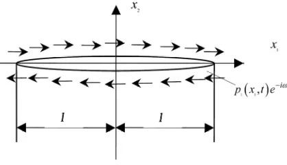
In this case the crack surfaces are subjected to the boundary conditions
2( ) 2( )
p x , t p x , t
for x (75)
2( ) 2( )
p x , t p x , t
for x , as it is shown in the Figure 1.
With considering contact interaction at the crack edges, the load vector on the crack edges has the form
2 1
2 1 2 1 1 ; 2 1
( , )
( , ) ( , ) , 0 ,
s
e
p x t
p x t q x t x q x
(76)
where e
is a region of close contact, which is varied during time.The force of contact interaction at the crack edges
2
Figure 1.Rectangular crack under normal loading.
2 2
uu should satisfy the contact constrains in the form
2 0 2 0 2 2 0 x ,
u , q , u q t
(77)
Loading p x t2( , )1 on the crack edges and their
open-ing u x t2( , )1 may be expanded into Fourier series
1
2( , )1 ( 2( ,1 k))
p x t F p x
,u x t2( , )1 F1(u x2( ,1 k))
(78) where
2( ,1 k) ( 2( , ))1
p x F p x t ,u x2( ,1 k) F( u x t2( , ))1
(79) Fourier series expansions of the displacement discon-tinuity 2( )
k
u
x and the traction 2( )
k
p x are related
by the BIE of the form
2( ) . . 22( , ) 2( )
k k
k
p F P F u d
x x y y ,
0, 1, 2, ,
k , x (80)
The kernels F22(xy,k) may be obtained from
fundamental solutions for the 2-D steady-state wave equations of elastodynamics, which is well known and may be find in [3,4,20].
This problem was solved using above four algorithms. Dependence of the algorithms convergence rate on wave number is presented in Figure 2. Analysis of these data shows that all algorithms are convergent and obtained results coincide for all algorithms, but convergence rate is different.
An analysis of results in Figure 2 reveals that Algo-rithm 3 and AlgoAlgo-rithm 4 have significantly faster con-vergence for all wave numbers.
8.2. Shear H-Wave
[image:8.595.310.536.81.230.2]Let harmonic shear H-wave with multiple frequencies propagates normally to the crack surface. The inci-dent wave is defined by the potential function
Figure 2. Convergence of the algorithms for different wave numbers.
2 2
( )
1
( , )t ei k xt
x , (81) where 1 is the amplitude of the incident wave,
2 / 2
k c is the wave number, c2 is the
ve-locity of the H-wave, 2 / T is the frequency. Following [3,4] we consider two separate problems: the problem for incident waves and the problem for re-flection waves. Obviously, in the case under considera-tion the problem for incident wave is trivial. Therefore we will pay attention to solution of the problem for the reflected waves.
The load on the crack’s edges caused by the incident waves has the form
*
1( ) Re{ 1( )1 }
i t
p x , t p x e , p1*k221 (82)
In this case the crack surfaces are subjected to the boundary conditions
1( ) 1( )
p x , t p x , t for x , (83)
1( ) 1( )
p x , t p x , t
for x , as it is shown in the Figure 3.
With considering contact interaction at the crack edges, the load vector on the crack edges has the form
1 1 1 1
1 1 1 ; 1 1
( , ) ( , )
( , ) , 0 ,
s
e
p x t p x t
q x t x q x
(84)
where e
is a region of close contact,which is varied during time.
The force of contact interaction at the crack edges q1
and displacement discontinuity (crack opening)
1 1 1
u u u
should satisfy the contact constrains in the form
1 2 1
1 2 1 1
0,
x ,
t
t
q k q u
q k q u q t
(85)
where k is a friction ration; t u1 q1 is a
Figure 3.Rectangular crack under shear loading.
a normal contact force, in the problem under considera-tion it is known before.
Loading p x t1( , )1 on the crack edges and their opening
1( , )1 u x t
may be expanded into Fourier series
1
1( , )1 ( 1( ,1 k))
p x t F p x 1
1( , )1 ( 1( ,1 k))
u x t u x
F
(86) where
1( ,1 k) ( 1( , ))1
p x F p x t , u x1( ,1 k) F( u x t1( , ))1
(87) In Guz and Zozulya 2001, 2002 it was shown that Fourier series expansions of the displacement disconti-nuity 1( )
k
u
x and the traction 1( )
k
p x are related by the BIE of the form
1( ) . . 11( , ) 1( )
k k
k
p F P F u d
x x y y ,
0, 1, 2, ,
k , x (88)
The kernels F11(xy,k) may be obtained from
fundamental solutions for the 2-D steady-state wave equ- ations of elastodynamics, which is well known and may be find in [3,4,20].
This problem was solved using above four algorithms. Dependence of the algorithms convergence rate on wave number is presented in Figure 4.
Analysis of these data shows that all algorithms are convergent and obtained results coincide for all algo-rithms and convergence rate is not differing significantly. Our calculations show that all four above algorithms are convergent in elastodynamic problems with contact and with friction for infinite cracked body. It is important to mention that Algorithm 3 and Algorithm 4 have signifi-cantly faster convergence in both cases frictionless con-tact problem and problem with friction.
9. Conclusions
[image:9.595.311.540.81.229.2]This paper present various variational formulations of elastodynamic problem for body with crack with consid-ering possibility for unilateral crack faces contact inter-action and friction. Variational formutations is based on boundary variational principle and on fundamental solu-
Figure 4. Convergence of the algorithms for different wave num- bers.
tions. Nonsmooth functionals that correspond to unilare-ral frictional contact conditions are constructed. Iterative algorithms of the Uzawa’s type that are based on projec-tion on the set of unilateral restricprojec-tions and fricprojec-tion are proposed. It was shown that in the case if varational formulation is based on principles formulated only for boundary the BIE method may be used. The case of the crack in infinite elastic media is considered in more de-tails and four new algorithms are proposed. To study convergence of the proposed algorithms two problems related to the crack faces contact interaction under action of the harmonic tension-compression and shear waves have been solved numerically using BIE method.
10. References
[1] V. V. Zozulya, “On Solvability of the Dynamic Problems in Theory of Cracks with Contact, Friction and Sliding Domains,” Doklady Akademii Nauk Ukrainskoy SSR, Vol. 3, 1990, pp. 53-55, in Russian.
[2] V. V. Zozulya, “Method of Boundary Functionals in Con-tact Problems of Dynamics of Bodies with Cracks,” Dok-lady Akademii Nauk Ukraine, Vol. 2, 1992, pp. 38-44, in Russian.
[3] A. N. Guz and V. V. Zozulya, “Brittle Fracture of Con-structive Materials under Dynamic Loading,” Naukova Dumka, Kiev, 1993, in Russian.
[4] A. N. Guz and V. V. Zozulya, “Fracture Dynamics with Allowance for a Crack Edges Contact Interaction,” In-ternational Journal of Nonlinear Sciences and Numerical Simulation, Vol. 2, No. 3, 2001, pp. 173-233.
[5] A. N. Guz and V. V. Zozulya, “Elastodynamic Unilateral Contact Problems with Friction for Bodies with Cracks,” International Applied Mechanics, Vol. 38, No. 8, 2002, pp. 895-932.
[7] V. V. Zozulya, “Mathematical Investigation of Non- smooth Optimization Algorithm in Elastodynamic Con-tact Problems with Friction for Bodies with Cracks,” In-ternational Journal of Nonlinear Sciences and Numerical Simulation, Vol. 4, No. 4, 2003, pp. 405-422.
[8] C. Polizzotto, “A Boundary Min – Max Principle as a Tool for Boundary Element Formulations,” Engineering Analysis with Boundary Elements, Vol. 8, No. 2, 1991, pp. 89-93.
[9] J. Cea, “Optimization,” Teorie et Algorithms, Dunod, Paris, 1971, in French.
[10] I. Ekeland and R. Temam, “Convex Analysis and Varia-tional Problems,” North-Holland, 1975.
[11] V. V. Zozulya, “Variational Principles and Algorithms in Contact Problem with Friction,” In: N. Mastorakis, V. Mladenov, B. Suter and L. J. Wang, Eds., Advances in Scientific Computing, Computational Intelligence and Applications, WSES Press, Danvers, 2001(a), pp. 181- 186.
[12] V. V. Zozulya, “Variational Principles and Algorithms in Elastodynamic Contact Problem with Friction,” In: S. N. Atluri, M. Nishioka and M. Kikuchi, Eds., Advances in Computational and Engineering Sciences, Technology Science Press, Puerto Vallarta, Mexico, 2001(b).
[13] V. V. Zozulya and O. V. Menshykov, “Use of the Con-strained Optimization Algorithms in Some Problems of
Fracture Mechanics,” Optimization and Engineering, Vol. 4, No. 4, 2003, pp. 365-384.
[14] V. V. Zozulya and M. V. Menshykova “Study of Iterative Algorithms for Solution of Dynamic Contact Problems for Elastic Cracked Bodies,” International Applied Me-chanics, Vol. 38, No. 5, 2002, pp. 573-577.
[15] V. V. Zozulya, “Fracture Dynamics with Allowance for Crack Edge Contact Interaction,” In: C. Constanda, P. Schiavone and A. Mioduchowski, Integral Methods in Science and Engineering, Birkhauser, Boston, 2002, pp. 257-262.
[16] V. V. Zozulya and P. Rivera, “Boundary Integral Equa-tions and Problem of Existence in Contact Problems with Friction,” Journal of the Chinese Institute of Engineers, Vol. 3, No. 3, 2000, pp. 313-320.
[17] N. Kikuchi and J. T. Oden, “Contact Problems in Elastic-ity,” SIAM Publications, Philadephia, 1987.
[18] P. D. Panagiotopoulos, “Inequality Problems in Mechan-ics and Applications, Convex and Non Convex Energy Functions,” Birkhauser, Stuttgart, 1985.
[19] A. C. Eringen and E. S. Suhubi, “Elastodynamics, Vol. 2. Linear Theory,” Academic Press, New York, 1975. [20] J. Dominguez, “Boundary Elements in Dynamics,”