doi:10.4236/ijis.2011.11001 Published Online July 2011 (http://www.SciRP.org/journal/ijis)
Using Intelligent Computational Methods for
Optimizing Niching Method
Mohsen Jahanshahi
Computer Engineering Department, Central Tehran Branch, Islamic Azad University, Tehran, Iran E-mail: [email protected]
Received June 22, 2011; revised July 18, 2011; accepted July 25, 2011
Abstract
Optimization implies the minimization or maximization of an objective function. Some problems have sev-eral optimum points which all, should be computed. Niching method is presented to do so. However, its effi-ciency can be improved via combining it with Memetic algorithm. Therefore, in this paper, Memetic method is used to improve this method in terms of convergence rate and diversity. In the proposed methods, genetic algorithm, PSO, and learning automata are used as a local search algorithm of Memetic method. The result of simulations demonstrates that proposed methods are more effective compared with Niching in terms of convergence and diversity.
Keywords:PSO, Niching, Genetic Algorithm, Learning Automata
1. Introduction
Optimization is the minimization or maximization of an objective function that normally is done with considera-tion of limitaconsidera-tions identifying condiconsidera-tions of a problem. In other words, it means the finding of the best solution for a given problem. Some problems have several local op-timums which may be computed using Niching method [1]. In this paper, memetic method is used for increase of convergence speed and also the increasing rate of parti-cles’ diversity in Niching method, as two assessment factors of search methods. In this research, genetic algo-rithms (GA) [2], particle swarm optimization (PSO) [3], and learning automata (LA) [4] are used as three local search algorithms in memetic method.
The rest of the paper is organized as follows. In sec-tion 2, PSO method is briefly introduced. In secsec-tion 3, NichePSO is discussed in summary. Section 4 explains used local search methods and then proposed methods are discussed in section 5. The results of simulations are included in section 6. Section 7 concludes the manu-script.
2. Particle Swarm Optimization
Particle swarm optimization (PSO) was discussed in [3] and then has been improved for many years. It is
com-bined by GA in [5] and modified in [6-8] work on dis-crete PSO as a new direction. PSO has been successfully utilized for aircraft transportation [9] and optimal path discovery in automated drilling operations [10], to name a few. There are also some other works which concen-trated on its functionality which are not in the scope of this manuscript [11,12].
The main idea of PSO had been taken from Birds or fishes swarm behavior which are searching for meal. Some birds are searching for meal randomly. Only a piece of meal may be found in the mentioned space. None of them knows about the real place of the meal. One of the best strategies is to follow a bird that is placed in minimum distance to a meal. In fact, this strategy is basis of PSO algorithm.
cur-rent position will continue its movement in the space of problem.
PSO starts in this way that a swarm of particles (solu-tions) are generated randomly and are updated during the generations and attempt to find an optimum solution. In each step, every particle is updated using two best values. First, is the best situation that a particle has ever been reached. It is known and kept by personal best (pbest). Another best value is used by the algorithm is the best position that has ever been obtained by a swarm of parti-cles. It is known by global best (gbest). In some PSO editions, a particle chooses parts of populations that are its topological neighbors and only involves those in its behavior. In this case, the best local solution is shown by
lbest (local best) and is used instead of gbest. After find-ing the best values, the velocity and position of particles are updated by formula (1) and (2) given below:
1* *
2 * *
-v v c rand pbest position
c rand gbest position
(1)
position position V (2) In (1) and (2) equations, V
is the particle velocity and position
is current position of a particle. Both are arrays as long as the number of problem dimensions.
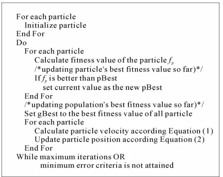
Rand is a random variable in the random domain. (0, 1) c1 and c2 are learning parameters, normally both are the same values as c1= c2 = c. In each dimension, veloc-ity of particles is limited to a Vmax. In case, the sum of accelerations cause that the velocity in one dimension exceeds the maximum value, it is considered as Vmax. The right hand side of Equation (1) is composed of three components, the first part, is the current velocity of a particle, the second and third parts take responsibility for variation of the velocity and its rotation towards the best personal and swarm experiences. Combining these two factors in Equation (1) helps create a balance between local and global searches. Let us we don’t consider the first part of the equation then the particles velocity is determined only with consideration of current position and the best single and swarm experiences of particles. Therefore, the best particle is fixed in its position and the rest of the particles move towards it. In fact, if we ignore the first part of Equation (1), PSO will be a process in which, search space gradually becomes smaller and local search is performed around the best particle. In contrast, if we consider only first part of the Equation (1), then the particles will continue their normal route up to border and it is said those are doing global search. Pseudo code of PSO algorithm is shown in Figure 1.
[image:2.595.315.534.76.250.2]Since in this algorithm, particles gradually tend to current optimum solution so if this is a local optimum solution then whole particles move towards it conse-
Figure 1. Pseudo code of PSO algorithm.
quently PSO is not a practical way to leave this local optimization. Meanwhile, some problems have more than one general optimum solution that all have to be computed. These are the greatest problems of PSO algo-rithm that make it unable to solve multi peak problems particularly with a large state space.
3. Niche PSO
Niche PSO is presented to find all the solutions of prob-lems with more than one general optimum solution [1]. In this algorithm, niches are parts of the environment and main operation of each niche is to self-organize the par-ticles to independent sub-swarm. Each sub-swarm de-termines the position of one niche and keeps it. The task of each sub-swarm is to find one of the optimum solu-tions. No information is exchanged amongst sub-swarms. This independency lets sub-swarms to keep niches. In summary, it can be said that performance of sub-swarms is stable and independent of the other swarms.
Niche PSO begins its operation with one swarm that is called main swarm that includes whole particles. As soon as, a particle gets close to an optimum solution, one swarm will be formed with classification of particles. Then these particles are put out of the main swarm and continue the operations for finding the solution in their own sub swarms. In fact the main swarm is broken into some sub-swarms. Niche PSO is convergent when smaller sub-swarms improve their presented solutions, and then in continue, the best global position for each sub-swarms is accepted as a solution. Pseudo code for Niche PSO is shown in Figure 2. Different steps of this algorithm are explained in details in section below.
3.1. Training Main Swarm
Create and initialize a nxdemensioal main swarm, S; Repeat
Train the main swarm, S, for one iteration using the cognition-only model;
Update the fitness of each main swarm particle, S x i;
for each sub-swarm Sk do
Train sub-swarm particle, Skxi, using a full model PSO;
Update each particle’s fitness;
Update the swarm radius SkR;
End for
If possible, merge sub-swarms;
Allow sub-swarms to absorb any particle from the main swarm that moved in to the sub-swarm;
If possible, create new sub-swarm;
Until stopping condition is true;
[image:3.595.370.478.73.143.2]Return Skˆy for each sub-swarm Sk as a solution;
Figure 2. Niche PSO algorithm.
and position of the particles.
3.2. Training Sub-Swarms
Sub-swarms are independent swarms. In this paper, for training those, local search methods are used such as genetic algorithms, memetic and PSO. Use of methods above for training sub-swarms improves this method.
3.3. Identification of Niches
When a particle is getting close to a local optimum, a swarm is formed. If the acceptability rate of a particle indicates tiny variation of some repetitions, then the swarm will be formed by this particle and its nearest neighbors. In simpler word, standard deviation (i)
oc-curs in some repetition in objective function (f x
i ) foreach particle. If (i), the swarm is formed. To
pre-vent the dependency problem, (i) is normalized based
on domain. The nearest neighbor of for position of (xi)
of particle i, is given by Euclidean distance as follow:
arg min i a a
l x x (3)
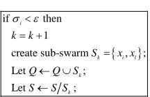
The process of swarm generation or niche identifica-tion is summarized in Figure 3. In this algorithm, the symbol Q indicates set of sub-swarms (Q
S1,,SK
)where, (Q K). Each sub-swarm has the number of (Skns) particles. At the time of Niche PSO generation,
the value of K is zero and Q is an empty set.
3.4. Absorbing Particles in Sub-Swarms
Particles of main swarm move towards an area that is covered by the sub-swarms (Sk). These particles
com-bine with sub-swarm for reasons below:
if then
1
create sub-swarm , ; Let ;
Let ;
i
k i l
k
k
k k
S x x
Q Q S
S S S
[image:3.595.58.290.78.273.2]
Figure 3. Generation algorithm of sub-swarms in Niche PSO.
The particles move in search area for creation of a sub-swarm may improve the diversity of sub-swarms.
These particles in a sub-swarm increase the dispersion of those to an optimum space via increase of general information.
If for particle i we have:
ˆ
i k k
x S y S R (4) Then the particle i is absorbed to sub-swarm (Sk) in
such a way
k k i
i
S S x
S S x
(5)
In equation above, ( SkR ) points to radius of
sub-swarm (Sk) and is defined as follow:
ˆ
max . . 1, ,
k k k i i k s
S R S yS x S n (6)
Here, ( Skyˆ ) is the best general position of sub-swarm (Sk).
3.5. Merging of Sub-Swarms
Perhaps, more than one sub-swarms points to an opti-mum point. Here, it is possible that a particle moves to a solution is not absorbed to a sub-swarms. As a result, a new sub-swarm will be generated and it leads to a prob-lem that a solution is followed by several sub-swarms in form of redundancy. For solving this problem, similar sub-swarms must merge together. The sub-swarms are the same if their space is considered in such a way that radiuses of particles converge in sub-swarms. The new merged sub-swarm has more general information and uses experiences of both old sub-swarms. The results of new sub-swarm are normally more accurate than the smaller old sub-swarm. In simpler word, two sub-swarms (Sk) and (Sk1) merge together if:
1 ˆ 2 ˆ 1 2
k k k k
S y S y S R S R (7) If (Sk1 R Sk2 R 0) the following formula will be
replaced with equation 8.
1 ˆ 2 ˆ
k k
S y S y (8) where µ is a tiny value tends to zero (e.g. 103
). If µ
solu-tions. In order to keep µ in the domain, ( Sk1 yˆ Sk2yˆ )
is normalized in (0, 1).
3.6. Stop Conditions
Several stop conditions may be used to finish the search of solutions. Note that each sub-swarm has founded a unique solution.
4. Used Local Search Method
We applied the PSO algorithm as a local search method in Memetic which was introduced in section 2. We have also utilized genetic algorithm and learning automata which are briefly introduced in the next sub-section.
4.1. Genetic Search Algorithm
Genetic algorithm was introduced by John Haland for the first time in 1975 and since then has been used for solv-ing optimization problems [2]. Genetic algorithms have great applications in random searches and optimization techniques. Today's those are known more as type of evolutional calculations. This algorithm is similar to natural evolution process and unlike the other methods, uses a population for search in solution space and always applies the principle “survival based on eligibility” to population. Based on this principle, after creation of every generation, unqualified chromosomes will be killed and eliminated from populations, only suitable chromosomes will be remained and create next genera-tion and make suitable solugenera-tions from those.
If genetic algorithm is designed well, all the popula-tion will converge to a unique global optimum solupopula-tion. Genetic algorithms are so powerful and effective and practical for problems with no systematic solutions.
4.2. Theory of Learning Automata
In this section the Learning Automata for the proposed framework will be briefly reviewed;
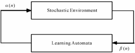
Learning automata (LA) is an abstract model that chooses an action from a finite set of its actions ran-domly and takes it [4,13]. In this case, environment evaluates this taken action and responses by a reinforce-ment signal. Then, learning automata updates its internal information regarding both the taken action and received reinforcement signal. After that, learning automata chooses another action again. Figure 4 depicts the rela-tionship between learning automata and environment. Every environment is represented by E{ , , } c , where
1, 2, , r
is a set of inputs,
1, 2,,r
[image:4.595.310.538.77.168.2]is a set of outputs, and c
c c1, 2,,cr
is a set of pen-Figure 4. Interaction between learning automata and envi-ronment.
alty probabilities. Whenever set has just two mem-bers, model of environment is P-model. In this environ-ment 11, 20 are considered as penalty and
reward respectively. Similarly, Q-model of environment contains a finite set of members. Also, S-model of envi-ronment has infinite number of members. ci is the
pen-alty probability of taken action i.
Learning automata is classified into fixed structure and variable structure. Learning automata with variable struc-ture is introduced as follows; Learning automata with variable structure is represented by
, , ,p T
, where
1, 2, , r
is a set of actions,
1, 2,,r
is a set of inputs, p
p p1, 2,,pr
is the actionprobability vector, and p n
1
T
n , n ,p n is learning algorithm. Learning automata operates as follows; learning automata chooses an action from its probability vector randomly (Pi) and takes it. Suppose
that the chosen action is i. Learning automata after
receiving reinforcement signal from environment updates its action probability vector according to formulas 9 and 10 in case of desirable and undesirable received signals respectively. In formulas 9 and 10, a and b are reward and penalty parameters respectively. If a = b then algo-rithm is named LR P . Also, if b a then the
algo-rithm is named LR P . Similarly, if b = 0 then the
algo-rithm is called LR I .
1 1
1
i i i
j j j
p n p n a p n
p n p n a p n j j i
(9)
1 1
1 1
1
i i
j j
p n b p n
b
p n b p n
r j j i
(10)
5. Proposed Methods
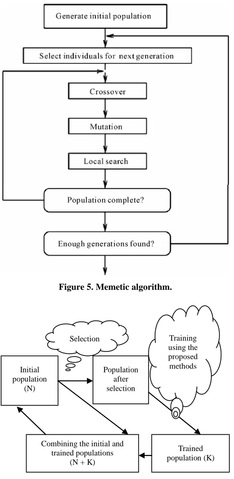
methods by Niche PSO for improvement of this method. In proposed methods in each sub-swarm, a set of parti-cles is chosen and improved by one of local search methods. Improved particles are added to set of whole particles and from those, enough sub-swarms will be chosen. The structure of memetic method and proposed method are shown in order, in Figures 5 and 6.
For training the particles inside each niche, genetic algorithm by training single particle, genetic by training several particles and PSO have been used.
[image:5.595.57.290.231.708.2]In continue, details of used algorithms are presented as a local search in memetic method.
Figure 5. Memetic algorithm.
Initial population
(N)
Population after selection
Trained population (K) Combining the initial and
trained populations (N + K)
Selection Training using the proposed methods
Figure 6. Proposed framework.
5.1. GA-Based Local Search Method
As described above, we have used GA as local search in Memetic method. Mutation operator of GA was done as follows. The best particle of sub-swarm is chosen and its value is converted to a binary number. Then Mutation is applied to it once, if the value of new particle is getting better the old one, new particle will be replaced with the old one. We name this method as GA1.
We also propose another GA-based method in which the Mutation operator was accomplished as follows. In each sub-swarm, one quarter of the particles are chosen randomly. Then single point Mutation is applied to each particle up to maximum three times. Each time if the generated particle is better than the old one, it will be replaced with the old one and next go to another particle. We call this method as GA2
5.2. PSO-Based Local Search Method
In this method, PSO algorithm is used as local search. This method is done in two ways: one global best (all the swarms) and another local best (inside the sub-swarm) that by global best method poor results are obtained.
5.3. LA (LR – P)-Based Method
This method uses learning automata to update the veloc-ity of particles. In this method two functions are consid-ered to update particles velocity by learning automata. The first operation means to consider the effect of global best of subgroup for updating a particle and the second operation means to update velocity of the particle with-out consideration of the global best of subgroup. After applying these functions to whole particles of subgroup if the total values of particles is less than the old total value of the particles then automata is rewarded other-wise is penalized.
5.4. LA (LR – I)-Based Method
This method is similar to method above. The only dif-ference is that after doing Automata functions on whole particles of subgroup, if the total values of current parti-cles is less than the old partiparti-cles then the automata is rewarded but if the total value of particles is more than old total values the automata is not penalized.
6. Simulation Results
Figure 7. Approaching the particles to the local optima.
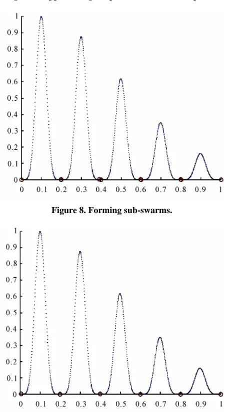
[image:6.595.309.540.573.703.2]Figure 8. Forming sub-swarms.
Figure 9. Full running of algorithm and combination of sub-swarms and reaching all the optimum solutions.
simulations is to find optimum points of a following standard function.
exp 2 log 2 2 0.08 0.854 2
sin 5 6
y x
pi x
(9)
In all simulations, PSO parameters are initially valued as follow:
1 1.2
c 0.01a r1 a barand
40
pop
2 1.2
c b1 r2 a barand
Also the value of inertia weight w is given by the fol-lowing formula where, T is the maximum repetition and t
is current time of simulation.
1
0.5 0.3
1
t w
T
(10)
Figures 7 to 9 shows the result of a sample of running algorithm and the process of reaching optimum solution for particles during simulation.
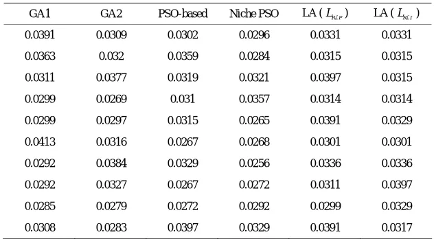
Figure 10, depicts the diversity rate of particles during different simulations. This results are gained from 10 times repetition of an algorithm that its accurate results is listed in Table 1 in which the values are gained by taking the mean of variance for whole particles during the pe-riod of each step of simulation. As depicted in this figure, the method LA (LR P )-based has the most diversity rate
and hence outperforms the others schemes. In this evaluation, LA (LR I )-based method stands in the
sec-ond place. Table 2 lists the divergences behavior of the proposed designs over the 50 runs. From the results, LA (LR I )-based method has the least divergence rate and
hence outperforms the other methods in terms of con-vergence rate.
7. Conclusions and Future works
In this paper, five combinational methods were presented
Table 1. Diversity rate of particles in various algorithms in 10 times of simulations.
GA1 GA2 PSO-based Niche PSO LA (LR P ) LA (LR I )
[image:7.595.139.455.94.268.2]0.0391 0.0309 0.0302 0.0296 0.0331 0.0331 0.0363 0.032 0.0359 0.0284 0.0315 0.0315 0.0311 0.0377 0.0319 0.0321 0.0397 0.0315 0.0299 0.0269 0.031 0.0357 0.0314 0.0314 0.0299 0.0297 0.0315 0.0265 0.0391 0.0329 0.0413 0.0316 0.0267 0.0268 0.0301 0.0301 0.0292 0.0384 0.0329 0.0256 0.0336 0.0336 0.0292 0.0327 0.0267 0.0272 0.0311 0.0397 0.0285 0.0279 0.0272 0.0292 0.0299 0.0329 0.0308 0.0283 0.0397 0.0329 0.0391 0.0317
Table 2. Divergence rate of different algorithms.
LA (LR I ) LA (LR P ) Niche PSO PSO-based GA2 GA1
5 11 12 15 8 12
to raise the diversity of particles and improvement of convergence of NichePSO as two assessment factors of search methods. From the results, LA (LR P )- and LA
(LR I )-based methods outperform other methods in terms
of diversity and convergence rates, respectively.
8. References
[1] R. Brits, A. P. Engelbrecht and F. van den Bergh, “A Niching Particle Swarm Optimizer,” Proceedings of the IEEE Swarm Intelligence Symposium, Indianapolis, 24 - 26 April 2003, pp. 54-59,
[2] P. Moscato, “Genetic Algorithms and Martial Arts to-wards Memetic Algorithm,” Calteth Concurrent Compu-tation Program Report 826, Moscato, 1989.
[3] J. Kennedy and R. C. Eberhart, “Particle Swarm Optimi-zation,” Proceedings of IEEE International Conference on Neural Networks, Piscataway, 27 November - 1 De-cember 1995, pp. 1942-1948.
[4] M. A. L. Thathachar and P. S. Sastry, “Varieties of Learning Automata: An Overview,” IEEE Transaction on Systems, Man, and Cybernetics-Part B: Cybernetics, Vol. 32, No. 6, 2002, pp. 711-722.
[5] A. Stacey, M. Jancic and I. Grundy, “Particle Swarm Optimization with Mutation,” Proceedings of the Con-gress on Evolutionary Computation, Canberra, 8 - 12 December 2003, pp. 1425-1430.
[6] Y. Shi and R. C. Eberhart, “A Modified Particle Swarm Optimizer,” IEEE International conference on Evolu-tionary Computation, Anchorage, 4 - 9 May 1998.
[7] M. Clerc, “Discrete Particle Swarm Optimization,” New Optimization Techniques in Engineering, Springer-Verlag, New York, 2004.
[8] P. Yin, “A Discrete Particle Swarm Algorithm for Opti-mal Polygonal Approximation of Digital Curves,” Jour-nal of Visual Communication and Image Representation, Vol. 12, No. 2, 2004, 241-260.
[9] G. Venter and J. Sobieszczanski-Sobieski, “Multidisci-plinary Optimization of a Transport Aircraft Wing Using Particle Swarm Optimization,” Structural and Multidisci-plinary Optimization, Vol. 26, No. 1, 2004, pp. 121-131. [10] G. C. Onwubolu and M. Clerc, “Optimal Path for
Auto-mated Drilling Operations by a New Heuristic Approach Using Particle Swarm Optimization,” International Journal of Production Research, Vol. 4, No. 3, 2004, pp.
473-491.
[11] F. Bergh and A. P. Engelbrecht, “A New Locally Con-vergent Particle Swarm Optimizer,” IEEE International Conference on Systems, Man and Cybernetics, Tunisia, 2002.
[12] T. I. Zohdi, “Computational Design of Swarms,” Interna-tional Journal for Numerical Methods in Engineering, Vol. 57, No. 15, 2003, pp. 2205-2219.