Online Full Text

(1)

Abstract—A multi-level dynamic multi-objective evolution algorithm (MDEA) is presented in this paper for multi-objective optimization problems(MOPs). This algorithm divides the whole evolution into four search stages dynamically according to the amount of nondominated individuals in the population, and different strategies are applied in different stages . The proposed algorithm is validated by some benchmark test problems. Compared with four other state-of-the-art multi-objective algorithms, MDEA achieves competitive results in terms of three quality indicators.

Index Terms—evolutionary algorithm, multi-objective optimization, hybrid progressive, nondominated solutions, quick select algorithm.

I. INTRODUCTION

Multi-objective problems(MOPs) often involve more than one objectives, and these objectives are often conflicting, being incomparable and non-commensurable with each other. Multi-objective optimization is applied to offer a set of trade-off solutions namely the Pareto optimal solutions set for the MOPs. Evolutionary algorithms(EAs) are a nature-spired search strategy based on the evolutionary theory which is inspired by Darwinian(i.e., the natural selection of evolution ), and are well suited for tackling MOPs because of their exploration and exploitation abilities to find multiple trade-off solutions in the search space.

The current MOEAs researches focus on the following aspects[1]-[3], such as improving the methods of assigning the fitness value, the strategy of maintaining diversity, as well as promoting the ability of local search, employing dynamic or fixed external population. Among these existing algorithms, NSGAII[4] (the improved version of nondominated sorting genetic algorithm), SPEA2[5] (improved version of strength Pareto EA), PESA-II[6]，(new

Manuscript received march 5, 2010. This work was supported in part by the Natural Science Foundation of China (grant no: 50775089 ), the National High Technology Research and Development Program(863 Program) of China (Grant no:2007AA04Z190，2009AA043301 ), and the National Basic Research Program (973 Program ) of China (grant no: 2005CB724100 ).

Guojun,Zhang. is State Key Laboratory of Digital Manufacturing Equipment & Technology , Huazhong University of Science & Technology, Wuhan 430074, China; (e-mail: [email protected]).

Guibing,Gao is State Key Laboratory of Digital Manufacturing Equipment & Technology , Huazhong University of Science & Technology, Wuhan 430074, China, on leave from School of Mechanical Engineering, Hubei University of Technology, Wuhan 430068, China (e-mail: [email protected]).

Gang,Huang.Corresponding author, is State Key Laboratory of Digital Manufacturing Equipment & Technology , Huazhong University of Science & Technology, Wuhan 430074, China; (e-mail: [email protected]).

Peihua,Gu is State Key Laboratory of Digital Manufacturing Equipment & Technology , Huazhong University of Science & Technology, Wuhan 430074, China, and is College of Engineering, Shantou University,Shantou China ,515063. (e-mail: [email protected]).

version of Pareto-archived evolution strategy), FPGA[7](a fast Pareto genetic algorithm), MOCell[8](a cellular genetic algorithm for multi-objective optimization) are the popular MOEAs. As we all know, the Human beings have different interests in different stages,during the evolution, in different stages，the focus should be different. However, most of these algorithms employed a fixed pattern and selection metric on the whole evolution, few of them adopted different patterns in different stages adaptively and dynamically. On the other hand, in the evolutionary process, more solutions tended to lie at the current trade-off front, for most of these solutions, there is no distinct selection advantage[9], without an adequate selection method, it is difficult to find better solutions in the search space. Therefore, an adaptive and dynamic pattern which we called MDEA is proposed to handle the complicated problems.The advantages of different algorithms，such as the well-known nondominated sorted mechanism, the external archive population, the crowding distance metric and the feedback metric are combined into MEDA.

The remainder of this paper is organized as follows: In section 2, some famous MOEAs are studied, and MDEA, our proposal for solving MOPs, are described; in section 3, several test problems are used to evaluate MDEA’s effectively by comparing with NSGAII,SPEA2, PESA-II and MOCell; Finally the main conclusion and suggestion of the further research is presented.

II. THE ALGORITHM

In order to find the characteristics of the different algorithms in different evolutionary stages and combine their advantages into a new model, four state-of-the-art multi-objective optimization algorithms are studied before the MDEA is presented.

A.Study of Convergence Behavior

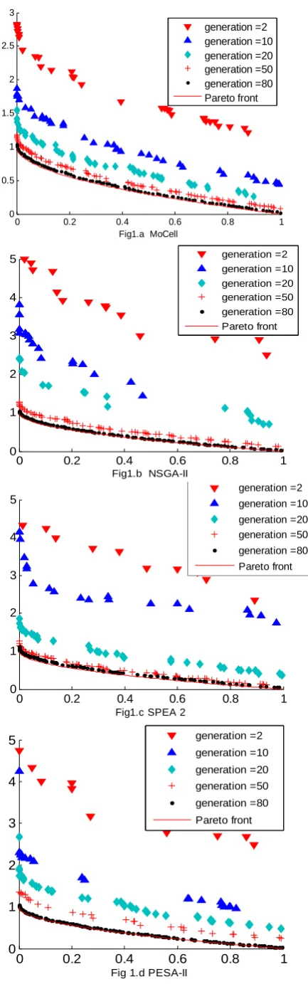
In order to find what should be focused on in different evolutionary stages, NSGAII , SPEA2, PESA-II and MOCell are studied to analyze the convergence behavior in different stages during the evolutionary process. Four typical convergence behaviors is obtained by MOCell, NSGAII, SPEA2 and PESA-II on test function ZDT1 are shown in Fig 1, and five different generations during the evolutionary stages are shown in the figures. Thirty independent runs are performed. The population size is 100, the crossover probability of pc=0.8, the mutation probability pm=0.01 and

the real-code mechanism is choosed. As shown in Fig 1, as the numbers of generation increase, the nondominated solutions continue to move towards the Pareto optimal front, and the solutions set is more closer to the pareto front. At the same time, there are slight differences in figures, while the number of generation is less than 20, the MOCell is easy to

MDEA: A Multi-level Dynamic Evolution

(2)

converge to a smaller value than other three algorithms, while

0 0.2 0.4 0.6 0.8 1

0 0.5 1 1.5 2 2.5 3

Fig1.a MoCell

generation =2 generation =10 generation =20 generation =50 generation =80 Pareto front

0 0.2 0.4 0.6 0.8 1

0 1 2 3 4 5

Fig1.b NSGA-II

0 0.2 0.4 0.6 0.8 1

0 1 2 3 4 5

Fig1.c SPEA 2

0 0.2 0.4 0.6 0.8 1

0 1 2 3 4 5

Fig 1.d PESA-II

[image:2.595.66.283.66.759.2]

Fig. 1. the Convergence trend in the evolution progress

the number gets up to 50, the NSGAII gets a more ideal value. As see from the above comparison, for the convergence

speed of the algorithm, there are differences in different stages, in the early stages, the MOCell’s convergence speed is faster than the others’,while in the later stages, the performance of NSGAII is the best among these four algorithms. In addition, we must point out that in the early stages of the evolution, the convergence speed of all the four algorithms are very fast and the amount of nondominated solutions increases sharply.

B.The Quantity of Nondominated Solutions in the Evolution

[image:2.595.310.516.405.559.2]

As we all know, these four MOEAs all have an external population to store the nondominated solutions found during the evolution. In Fig 2, the average ratio of nondominated solutions in external archive population found by MOCell, NSGII, SPEA2, PESA-II on ZDT1 in the evolutionary process are presented. Obviously, as the amount of nondominated solutions in the external population increases sharply when the number of generation is less than 80, in this stage, the emphasis of the algorithm is to search and select the nondominated solutions from the population, different strategies are applied in different algorithms and that is the key of the algorithm, how to improve the efficiency of search and selection is more important because the search and selection occupied much of the running time. When the number of generation is larger than 80, the amount of nondominated solutions in the archive population is equal to the population size, so the determination of whether or not the new nondominated solutions found by the algorithmare better than the existed nondominated solutions becomes the primary issue.

Fig. 2. the numbers of nondominated solutions found in the evolution progress

C. the Global Exploration Ability

Four typical snapshots of the different algorithms in initial stages on test function ZDT1 (30 dimensions) are shown in Fig 3. In general, during the early stages, the emphasis should be on the global exploration ability in the search space, the dispersity of individuals should be wider. For the SPEA2, we can see that some of the dominated solutions gathered in the middle space, this would be result in premature, For the MoCell and PESA-II, there are few solutions in the two endpoints, so the bound exploration ability would be worse than NSGA-II, based on this argument, it can be concluded that the NSGAII has a better early global exploration ability than the other three multi-objective optimization algorithms.

D. the Qucik Select Algorithm(QSA)

(3)

0 0.2 0.4 0.6 0.8 1 1

2 3 4 5 6

Fig 3.a MoCell

nondominated solutions dominated solutions

0 0.2 0.4 0.6 0.8 1

1 2 3 4 5 6

Fig 3.b NSGA-II

nondominated solutions dominating solutions

0 0.2 0.4 0.6 0.8 1

1 2 3 4 5 6

Fig 3.c SPEA2

nondominated solutions data2dominated solutions

0 0.2 0.4 0.6 0.8 1

1.5 2 2.5 3 3.5 4 4.5 5

PESA-II

nondominated solutions dominated solutions

Fig. 1. nondominated and dominated solutions compared in first generation about four different algorithms

(X Y ), the second is Y dominated X (X Y), the third is X=Y ,and the last is irrelevant (X doesn’t dominated Y,and Y doesn’t dominated X ). Motivated by the idea of three-way radix quicksort [22][ 23], and based on the relationshipof the

individuals in the population, an improved quick select algorithm is devised to select the nondominated solutions from the population, and the improved process is describled as follow: for each loop around, step 1: a radix individual

x

_i

is selected randomly from the external population to compare with the individuals which are in the evolution population, then the evolution population is divided into three sections, the front section are the individuals that are dominated by the

x

_i,the last section are individuals that dominated or equal to

x

_i , and the middle section is the individuals that is irrelevant with

x

_i, if

x

_idominates all the individuals in the evolution population, the search will stop and the evolutionary operation continue. Step 2: delect the front section and select a radix

x

_j in the last section randomly to compare with the individuals in the middle and last sections, again divide them into three sections, if

x

_j dominates all the other individuals, remove it to the archive population. Repeat step 2 until the front part is empty, now all the individuals left in the array are nondominated individuals and they will be copied to the archive population, if the archive population is full, the improved crowding distance, which is based on niche technique[5], is used to delete the individuals which have a worse crowding distance value.

This quick select algorithm can reduce the comparison among the dominated individuals, for example,N₁N₂,

1 3

N  N , N₁ N₄,if N₁ is the radix, then N₂,N₃,N₄ are

arranged in the front of N₁, and the comparison among them

are ignored in the next loop.

E. the Multi-Level Dynamic Evolution Algorithm

In this section, an improved multi-objective optimization algorithm, MDEA is described. MDEA is inspired by natural phenomenons: human’s growing process from birth to death could be divided into childhood, young, adolescent and old stages, while for the silkworms and snakes, each new exuviation represents the start of a new growth stage. MDEA is a population based evolutionary algorithm, a real-coded is implemented to avoid the difficulties associated with binary representation and bit operations, according to the solutions in the external population, the evolution of MDEA is divided into four different stages, gradually moving to the pareto front, during each stage, some excellent strategies which are used in others MOEAs are adopted to improve the efficiency of the algorithm.

(4)

RNSP(ratio of the nondominated solutions in population), an important parameter is introduced to distinguish whether the evolution is staying in this stage or not, if the RNSP is larger than 15%, the evolution steps to stage two.

Stage two: Stage two refers to the case that the RNSP is larger than 15%. As there are more nondominated solutions than stage one in the population, the emphasis in this stage is to improve the select efficiency. At the same time, in this stage the nondominated solutions found in the evolution are protected, so the external archive population is used to store the nondominated solutions during the search, following the scheme applied by SPEA2[6], and The QSA is used to select the nondominated solutions during the search.

Here, the external population metric used in SPEA2 is introduced to preserve the nondominated solutions found in the search from being destroyed, and QSA is devised to improve the efficiency of the selection, the hybrid model in stage two aims at maintaining the trade-off between the explorations ability of SPEA2 and the efficiency of the QSA, it is crucial to the whole algorithm.

The second important parameter called RNSEP (ratio of the nondominated solutions in external population) is used to dedicate whether the evolution is lingering in this stage or not, if the RNSEP is larger than 60%, the evolution steps to stage three.

Stage three : stage three refers to the case that the RNSEP is larger than 60%, the amount of nondominated solutions in the population increase sharply. The emphasis in this stage is to improve the bound exploration ability of the algorithm. So a feedback mechanism which is used in the MOCell is employed to improve the the border exploit capability, during each evolution, select nf nondominated solutions in the

external population randomly to the evolution population and replace the individuals which have a worse fitness value, the details see the references 9. If the value of RNSEP is equal to 100%, the evolutionary process steps to stage four, otherwise it continues stage three.

Stage four: Stage four refers to the case that the value of RNSEP is equal to 100%, which means that the archive is full of nondominated solutions. In this stage the improved crowding distance[5] is used to allocate the computational budget to do heuristic search. When the nondominated solutions found in the evolution dominate any of the solutions in the external archive population or they have a better crowding distance value than the nondominated solutions in the archive population, they will be plugged in and substitute for the bad ones. The key of this stage is to preserve the diversity of the nondominated solutions and to speed up the convergence.

The Details of MDEA are described as follows: Input : base parameters ( Pc,Pm , np0, npa ,nf,etc)

Output : nondominated solutions .

step1. Initialize all decisive parameters to user-specified values;

step2. Generate P0 individuals in the first generation;

step3. Run stage 1, rank the individuals with the fitness value, select pairs of individuals as parents from the previous population P0, perform the reproduction,crossover and

mutation operations to generate the offsprings and evaluate their fitness, if the fitness value is larger than the parents, delete the parents and add the offsprings into the population, otherwise just delete the offsprings. Finally the RNSP is

calculated, if its value is larger than 15%, turn to the step 4, otherwise continue the step3

Step4. Run stage 2, open the external archive population Pa, continue the evolutionary operations, and use QSA to

select the nondominated solutions from evolution population Pt to the Pa after each evolution, then the RNSEP is calculated,

if the value is larger than 60%, turn to the step 5,otherwise keep on the step4.

Step5. Run stage 3, select nf individuals in Pa randomly to

replace the individuals in Pt which are dominated by the

selected individuals, then continue the evolution operations. After each evolution, select the nondominated individuals to Pa, if the archive population is full, turn to the step 6,

otherwise continue step 5.

Step6. Run stage 4, calculate the crowding distance of solutions in Pa, add the better individuals found in the

evolution to the Pa and delete the individuals with bad

crowding distance.

Step7. Terminate the search if the stopping criterion is met; otherwise, return to Step 6 and continue.

III. EXPERIMENT

This section is devoted to evaluate the MDEA. A number of well-known benchmark multi-objective test problems are selected from the standard literature on EMO, such as Schaffer[19],Fonseca[20],Kursawe[21], as well as some complicated problems like the ZDT family problems[14], (noted:ZDT1,ZDT2,ZDT3,ZDT4, ZDT6 are selected) and the DTLZ family problems [13], (noted :for the DTLZ family problems, DTLZ1,DTLZ2, DTLZ3, DTLZ4, and DTLZ5 are selected, and the amount of objectives function is three ).

A. Quality Indicator

To evaluate the performance of an algorithm on the test problems, three quality indicators are used to measure the convergence behavior and diversity of solutions. Generation Distance[25] is applied to measure the convergence performance of the algorithm; Spread[14] is used to measure the diversity of the solutions set; Hypervolume ratio metric[13] is employed for the evaluation of both the convergence performance and diversity of the solutions. To determine these issues, it is necessary to know the exact location of the true Pareto Front, and for most of the benchmark problems used in this work, their Pareto Front have been obtained by using enumeration search strategy [26].

Generational Distance(GD ).

Van Veldhuizen and Lamont[25] applied this metric to evaluate the convergence behavior, it calculates how far the elements in the sets of nondominated solutions found by the algorithm from those in the known Pareto optimal sets. it is defined as:

n 2 i i 1

d

n

G D  

 ₍₂₎

(5)

convergence ability, and GD =0 indicates that all Pareto-optimal solutions found by the algorithm are in the Pareto-Front. The nondominated solutions set is normalized to guarantee a reliable result before calculating the GD.

Spread (Δ)

This metric is based on the calculation of the Euclidean distance between two consecutive nondominated solutions. Deb[14] applied this metric to measure the diversity of the solutions in two-objective problems. It is defined as:

1

f i = 1

f

d d d d

d d ( 1)

N i N d         



  (3) Where

d

_iis the Euclidean distance between consecutive solutions,

d

is the mean of these distances,

d

_fand

d

_l are the maximum and minimum Euclidean distances from the two extreme Pareto solutions to the closest nondominated solutions. But this metric is working only for the 2-objective problems, A.J.Nebro extended this metric for m-objective problems based on the modification proposed in[10], it is defined as: i= 1 1 ( , ) ( , ) ( , ) m i X S m i i

d e S d X S d

d e S S d

       



(4) 2 ,

( , ) min ( ) ( )

Y S Y X

d X S F X F Y

 

  , 1 _{( , )}

X S

d d X S

S _ 





Where m is the numbers of objectives, S is the set of solutions,

S

is the Pareto solutions,

(

e

₁



e

m

)

are the m extreme

solutions in

S

.

0  

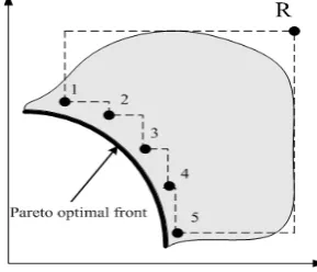
is the ideal distribution, that means a perfect spread out of the solutions in the Pareto Front. We also applied this metric to evaluate the diversity of the solutions.

[image:5.595.103.248.450.574.2]

Fig. 2. The hypervolume enclosed by the nondominated solutions

Hypervolume Ratio

Hypervolume metric is introduced by Zitzler and Thiele [13], the method is to calculate the volume of objective space covered by the nondominated solutions sets Q with the reference point R,(as shown in Fig 4, the region is enclosed by the discontinuous line, Q={1,2,3,4,5}).

( ) ( )

T F

H V N P H V R

H V P

 (1)

1

(NP )T _iQ i

HV volume v

    _ _   f 1

(PF) P i

i

HV volume v



 

 _ _

 ₍₂₎

Where Q is the nondominated solutions set found by the algorithm,

P

Fis the Pareto Front which is obtained by using

enumeration search strategy. HVR returns values in rang

[0,1], and a larger value of HVR obtainted by the algorithm is desirable.

B.Experimental result

For the test samples, the experimental results of the three quality indicatorsobtained by the MDEA, NSGAII,SPEA2, PESAII and MOCell are shown in table1,2&3. For each test problem, the median,

x

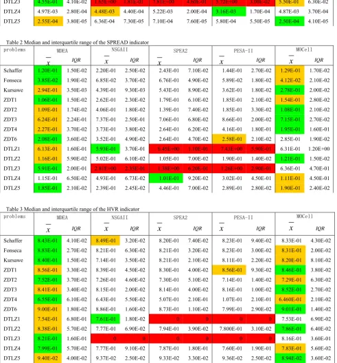
, and interquartile range, IQR, are listed in the tables, the best value for each problem is marked with green background while the second best value marked with yellow background.

In reference to the GD, the lowest value means that the resulting Pareto Front are closest to the true Pareto front, in table 1 it can be see that MDEA obtained the best performance in 6 of the 13 test MOPs and MOCell got the best values in 4 problems, while NSGAII obtained the best results in DTLZ1 and SPEA 2 obtained the best result in ZDT1, PESA-II obtained the best value in DTLZ4, that means in convergence for the five algorithms, the MDEA and MOCell did better than NSGAII, SPEA2,and PESA-II. Of course we must point out that in most cases the difference in GD values got by the different algorithms are very little, that indicates all the algorithms have the similar ability to compute the accurate Pareto front.

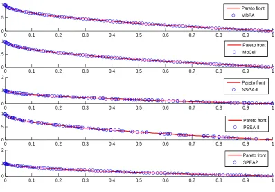
In terms of the spread (Δ), the lowest value means that the diversity of the solutions got by the corresponding algorithm is the best, from table 2, it is clear that MDEA obtained the best results in 6 of the 13 test problems while MoCell got the best results in 5 problems, NSGAII and SPEA2 yielded the best value only 1 problem respectively. To illustrate this fact graphically, the simulation results of ZDT1 obtained by five algorithms respectively are shown in Fig.5, obviously, MDEA obtained a better spreadout solutions than NSGA-II,SPEA2 and PESA-II, the non-dominated solutions found by MDEA achieved an almost perfect distribution along the Pareto front.

Finally, with regard to the HVR indicator, the measure of both the convergence and the diversity, the HVR metric should prove the results of the two other metric, the larger value of HVR obtained by the algorithms, the better the corresponding algorithm is. As we can see from table 3, MDEA obtained the best results in 7 of the 13 test problems while MoCell got the best results in 5, NSGAII yielded the best value in 1 DTLZ1 problem. From the comparison we can see that MDEA outperformed the other four algorithms.

On the other hand, we can see from table 3, SPEA2 and PESA-II yield a value of zero on the DTLZ1 and DTLZ3 while NSGA-II yield a value of zero on the DTLZ3, which means that they can’t convergence to the true Pareto Front of the problems.

Overall, considering the results of the experiments, we believe that the MDEA algorithm is a novel and efficient algorithm in solving MOPs because it obtained the competitive values in most test problems and it performed very stablly in terms of convergence, diversity or both.

C. the Running Time of the Algorithms

(6)

0 0.1 0.2 0.3 0.4 0.5 0.6 0.7 0.8 0.9 1 0

0.5 1

0 0.1 0.2 0.3 0.4 0.5 0.6 0.7 0.8 0.9 1

0 0.5 1

0 0.1 0.2 0.3 0.4 0.5 0.6 0.7 0.8 0.9 1

0 1 2

0 0.1 0.2 0.3 0.4 0.5 0.6 0.7 0.8 0.9 1

0 0.5 1

0 0.1 0.2 0.3 0.4 0.5 0.6 0.7 0.8 0.9 1

0 1 2

Pareto front NSGA-II

Pareto front MoCell

Pareto front PESA-II

[image:6.595.114.512.66.343.2]

Pareto front SPEA2 Pareto front MDEA

Fig 5 MDEA fin better solutions than NSGA-II,PESA-II,SPEA2

Fig. 6. running time of the different algorithm on 5 test problems

presented in Fig 6. The results are based on the experimental setting metioned above. We can observe from Fig 6, the test problems, the MoCell occupied the least running time while the SPEA2 was on the contrary, this may be resulted from the different strategies: MoCell makes use of parallelism [9], while SPEA2 makes use of an expensive archive truncation procedure whose worst run-time complexity is_{O n}

 

3 _[14].

Though archive population is hybridized in MDEA, the running time of MDEA is markedly less than that of NSGAII, SPEA2, because MDEA applied the QSA to construct the archive nondominated population, whose best running time complexity is  _N l o g N _ and worst run-time complexity

is Ο

 

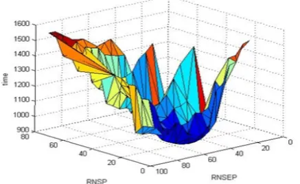
N2 [23]

D.Running Time Sentivity to the RNSP and RNSEP Parameters in MDEA

The impact of the parameters RNSP & RNSEP in MDEA are studied in this section. The test problems DTLZ1 and ZDT1 are adopted for parameters analysis because of their

complexity. Figure 7 shows the average running time versus RNSP &RNSEP parameters. The value of RNSP is at the range [0.1,0.8] while the value of RNSEP is at the range [0.20,1].The value of RNSP is smaller than that of RNSEP, as the RNSP is the demarcation between the stage one and stage two while the RNSEP is the demarcation between stage two and stage three. The range of [0.1,0.8] is adequate for RNSP, because if its value is less than 10%, the first stage won’t work.From Fig 7, we can see that when RNSP and RNSEP are both small or large, MDEA keeps a long running time, only when RNSP is range in [15%-30%] and RNSEP is range in [50%-65%], MDEA keeps a shorter running time. The reason may be as follows: when the RNSP is large, the stage one employed NSGA-II to do exploration in the objectives space, it will take relatively long time to search the nondominated solutions; when RNSEP is large, the QSA in stage two will take more time to select the nondominated solutions. therefore, to improve the efficiency or reduce the running time of MDEA,the value of RNSP should not be too large, and the value of RNSEP should be at a reasonable value, here 15% for RNSP and 55% for RNSEP are appropriate value for them.

IV. CONCLUSION

[image:6.595.77.282.393.522.2]

(7)

Table 1 Median and interquartile range of the GD indicator

problems _MDEA _NSGAII _SPEA2 _PESA-II MOCell

IQR IQR IQR IQR IQR

Schaffer 2.35E-04 2.12E-04 2.32E-04 1.71E-05 2.31E-04 1.53E-05 2.39E-04 1.20E-05 2.33E-04 1.78E-05 Fonseca 1.65E-04 1.45E-06 4.60E-05 4.71E-05 3.25E-04 3.40E-05 2.22E-04 2.40E-05 2.01E-04 2.70E-05

Kursawe 1.33E-04 1.10E-05 2.08E-04 3.80E-05 1.21E-04 1.90E-05 2.59E-04 2.20E-05 1.36E-04 1.40E-05 ZDT1 1.51E-04 2.33E-05 1.88E-04 4.43E-05 1.59E-04 1.45E-05 1.60E-04 1.76E-05 1.53E-04 3.76E-05

ZDT2 5.08E-04 7.40E-05 6.21E-04 4.67E-05 6.27E-04 3.24E-05 5.85E-04 4.56E-05 5.06E-04 5.67E-05 ZDT3 2.02E-04 9.45E-05 2.10E-04 1.85E-05 2.33E-04 2.41E-05 3.11E-04 2.50E-05 1.95E-04 2.25E-05

ZDT4 5.33E-04 1.24E-05 5.28E-04 7.63E-05 5.74E-04 2.90E-05 6.27E-04 5.02E-05 5.40E-04 5.90E-05 ZDT6 5.42E-04 2.00E-05 5.62E-03 5.30E-05 8.20E-04 7.30E-05 5.48E-04 2.50E-05 5.51E-04 1.80E-05 DTLZ1 2.14E-04 8.10E-05 1.81E-04 2.60E-05 1.82E+00 1.80E+00 3.63E-04 5.10E-05 4.52E-04 7.10E-05

DTLZ2 7.38E-04 4.90E-05 1.26E-04 2.30E-05 1.83E-04 4.70E-05 1.77E-04 4.10E-05 7.29E-04 6.80E-05 DTLZ3 4.55E-01 4.10E-02 1.65E+00 1.81E-01 7.81E+00 4.60E-01 5.72E+00 3.00E-02 5.50E-01 6.30E-02

DTLZ4 4.97E-03 2.80E-04 4.48E-03 4.40E-04 5.22E-03 2.00E-04 3.16E-03 1.70E-04 4.87E-03 3.70E-04 DTLZ5 2.55E-04 3.80E-05 6.36E-04 7.30E-05 7.10E-04 7.60E-05 5.80E-04 5.50E-05 2.50E-04 4.10E-05

Table 2 Median and interquartile range of the SPREAD indicator

problems _MDEA NSGAII _SPEA2 _PESA-II MOCell

Schaffer 1.20E-01 1.50E-02 2.20E-01 2.50E-02 2.43E-01 7.10E-02 1.44E-01 2.70E-02 1.29E-01 1.70E-02 Fonseca 3.85E-02 1.90E-02 6.85E-02 3.70E-02 6.76E-01 4.90E-02 5.89E-02 1.80E-02 4.12E-02 2.10E-02 Kursawe 2.94E-01 3.50E-03 4.39E-01 9.30E-03 5.43E-01 8.90E-02 3.62E-01 1.80E-02 2.78E-01 2.00E-02

ZDT6 2.08E-01 3.60E-02 3.52E-01 4.90E-02 2.64E-01 4.70E-02 2.58E-01 2.10E-02 2.85E-01 1.90E-02 DTLZ1 6.13E-01 1.60E-01 5.93E-01 3.70E-01 6.45E+00 1.10E-01 7.43E+00 5.90E-01 6.31E-01 1.20E+00 DTLZ2 1.16E-01 5.90E-02 5.02E-01 6.10E-02 1.05E-01 7.00E-02 1.90E-01 1.40E-02 1.21E-01 1.50E-02

DTLZ3 5.91E-01 2.00E-01 2.81E+00 2.35E-01 1.38E+00 6.20E-01 1.26E+00 2.90E-01 6.36E-01 4.70E-01 DTLZ4 1.15E-01 6.50E-02 4.93E-01 6.73E-02 1.01E-01 9.20E-02 3.02E-01 4.50E-01 1.11E-01 4.50E-01

[image:7.595.54.546.241.770.2]

DTLZ5 1.85E-01 2.10E-02 2.39E-01 2.45E-02 4.46E-01 7.00E-02 2.89E-01 2.80E-02 1.90E-01 2.40E-02

Table 3 Median and interquartile range of the HVR indicator

problems _MDEA _NSGAII _SPEA2 _PESA-II MOCell

Schaffer 8.43E-01 4.10E-02 8.49E-01 3.20E-02 8.20E-01 7.40E-02 8.23E-01 9.40E-02 8.33E-01 4.30E-02 Fonseca 8.83E-01 2.70E-02 8.21E-01 6.30E-02 8.21E-01 3.20E-02 8.23E-01 3.00E-02 8.31E-01 2.00E-02 Kursawe 8.40E-01 1.50E-02 7.14E-01 3.50E-02 8.21E-01 2.10E-02 8.11E-01 2.20E-02 8.20E-01 8.10E-02

ZDT3 8.41E-01 3.40E-02 8.15E-01 2.00E-02 8.14E-01 4.00E-02 8.16E-01 1.00E-02 8.52E-01 2.70E-02 ZDT4 6.55E-01 6.10E-02 6.43E-01 5.50E-02 5.07E-01 2.10E-01 1.07E-01 2.10E-01 6.460E-01 2.10E-02 ZDT6 9.00E-01 1.80E-02 8.86E-01 1.60E-02 8.73E-01 1.10E-02 7.99E-01 2.90E-02 9.01E-01 1.40E-02

DTLZ1 7.54E-01 6.80E-01 7.61E-01 1.80E-02 0 0 0 0 7.53E-01 6.90E-02 DTLZ2 8.38E-01 5.70E-02 7.77E-01 6.90E-02 7.94E-01 3.90E-02 7.800E-01 3.10E-02 7.86E-01 6.40E-02

DTLZ3 8.21E-01 1.60E-01 0 0 0 0 0 0 8.16E-01 3.60E-01 DTLZ4 7.99E-01 5.70E-02 7.77E-01 9.10E-02 7.87E-01 1.80E-01 7.60E-01 1.90E-01 7.83E-01 5.60E-02

DTLZ5 9.40E-02 4.00E-02 9.37E-02 2.50E-02 9.33E-02 3.30E-02 9.36E-02 2.50E-02 8.94E-02 3.60E-02

x

(8)

[image:8.595.52.271.65.199.2]

Fig. 7. running time versus parameters RNS on solving ZDT1 and DTLZ1by MDEA is a competitive and effective method considering the convergence and diversity measures.

A matter of future work is the application on solving the real-world problems. In this sense,we intend to employ MDEA to solve complicated problems in the multi-shop scheduling with mixed messages.

REFERENCE

[1]. Coello C.A.C. Evolutionary multiobjective optimization: A historical view of the field. IEEE Computational Intelligence Magazine, 1; 2006.pp 28–36.

[2]. Yao xin, Xu yong. Recent Advance in Evolutionary Computer. Computer science & technology 2006.pp 1-18

[3]. Coello C.A.C., and G.B. Lamont. Applications of Multi-Objective Evolutionary Algorithms. Singapore: World Scientific. 2004. [4]. Deb K., A. Pratap S. Agarval and T.A. Meyarivan. Fast and Elitist

Multiobjective Genetic Algorithm: NSGA-II. IEEE Transactions on Evolutionary Computing 6, 2002. pp 182 197.　

[5]. Zitzler E., M. Laumanns and L. Thiele. SPEA2: Improving

the Strength ParetoEvolutionary Algorithm. Technical Report 103, Computer Engineering and Networks Laboratory (TIK), Swiss Federal Institute of Technology (ETH) Zurich, Gloriastrasse 35,CH-8092 Zurich, Switzerland. 2001

[6]. CORNE D. W., N. R. JERRAM, J. D. KNOWLES, and M. J. OATES. PESA-II: Region-based selection in evolutionary multiobjective optimization. In Proceedings of the Genetic and Evolutionary Computation Conference (GECCO-2001), Morgan Kaufmann Publishers, San Francisco, CA, 2001.pp 283–290. [7]. H. Eskandari, C.D. Geiger, and G.B. Lamont. FastPGA: A Dynamic

Population Sizing Approach for Solving Expensive Multiobjective Optimization Problems. the 4th International Conference on Evolutionary Multi-Criterion Optimization, volume 4403 of Lecture Notes in Computer Science, 2007. pp 141–155.

[8]. A.J. Nebro, J.J. Durillo, F. Luna, B. Dorronsoro, E. Alba . MOCell: A Cellular Genetic Algorithm for Multiobjective Optimization. INTERNATIONAL JOURNAL OF INTELLIGENT SYSTEMS, VOL. 24, 2009 . pp 726–746.

[9]. A.J. Nebro, J.J. Durillo, F. Luna, B. Dorronsoro, E. Alba . AbYSS: Adapting Scatter Search for Multiobjective Optimization. Technical Report ITI-2006-2, Departamento de Lenguajes y Ciencias de la Computación, University of Málaga, E.T.S.I. Informática, Campus de Teatinos, 2006.

[10]. Nebro, A.J., Durillo, J.J., Coello Coello, C.A., Luna, F., Alba, E.: A Study of Convergence Speed in Multi-objective Metaheuristics. In: Rudolph, G., Jansen, T., Lucas, S., Poloni, C., Beume, N. (eds.) PPSN LNCS, vol. 5199, 2008. pp 171–185.

[11]. Durillo, J.J., Nebro, A.J., Luna, F., Dorronsoro, B., Alba, E.: jMetal: A Java Framework for Developing Multi-Objective Optimization

Metaheuristics. Tech. Rep. ITI-2006-10, Dept. de Lenguajes y Ciencias de la Computación, University of Málaga 2006

[12]. DEB, K.,A. PRATAP, S. AGARWAL, and T.MEYARIVAN. A fast and elitist multiobjective genetic algorithm: NSGA-II. IEEE Transactions on Evolutionary Computation, 6, 2002a. pp:182–197. [13]. DEB, K., L. THIELE, M. LAUMANNS, and E. ZITZLER. Scalable

multi-objective optimization test problems. In Proceedings of Congress on Evolutionary Computation, Honolulu, HI, IEEE Service Center, 1, 2002b. pp 825–830.

[14]. KHARE, V., X. YAO, and K. DEB. Performance scaling of multi-objective evolutionary algorithms. the Second International Conference on Evolutionary Multi-Criterion Optimization, Faro, Portugal, Springer-Verlag, Lecture Notes in Computer Science, 2632, 2003. pp 376–390.

[15]. S. Huband, L. Barone, R. L. While, and P. Hingston, “A scalable multiobjective test problem toolkit,” in EMO 2005, ser. LNCS, C. Coello, A. Hern´andez, and E. Zitler, Eds., vol. 3410, 2005. pp 280–295.

[16]. Cello C. A.C, G. T. PULIDO, and M. S. LECHUGA. Handing multiple objectives with particle swarm optimization. IEEE Transactions on Evolutionary Computations, 8, 2004. pp 256–279. [17]. J. Schaffer, “Multiple objective optimization with vector evaluated

genetic algorithms,” in First International Conference on Genetic Algorithms, J. Grefensttete, Ed., Hillsdale, NJ, 1987. pp 93–100. [18]. C. Fonseca and P. Flemming, “Multiobjective optimization and

multiple constraint handling with evolutionary algorithms - part II: Application example,” IEEE Transactions on System, Man, and Cybernetics, vol. 28, 1998.pp 38–47.

[19]. F. Kursawe, “A variant of evolution strategies for vector optimization,” in Parallel Problem Solving for Nature, H. Schwefel and R. M¨anner,Eds. Berlin, Germany: Springer-Verlag, 1990, pp 193–197.

[20]. E. Zitzler, K. Deb, and L. Thiele, “Comparison of multiobjective evolutionary algorithms: Empirical results,” Evolutionary Computation, vol. 8, no. 2, 2000. pp 173–195

[21]. Kalyanmoy Deb ,Santosh Tiwari . Omni-optimizer :A generic evolutionary algorithm for single and multi-objective optimization, European journal of operational research 185, 2008 pp 1062-1087 [22]. Jon L. Bentley and Robert Sedgewick, Fast Algorithms for Sorting

and Searching Strings, Proc. 8th Annual ACM-SIAM Symposium on Discrete Algorithms (SODA), 1997. pp 360-369,.

[23]. Srinivasan, D., Rachmawati, L.: An Efficient Multi-objective Evolutionary Algorithm with Steady-State Replacement Model. In: Genetic and Evolutionary Computation - GECCO 2006, pp 715–722 [24]. Huband, S., Hingston, P., Barone, L., While, R.L.: A review of multiobjective test problems and a scalable test problem toolkit. IEEE Trans Evolutionary Computation 10(5), 2006. pp 477–506 [25]. Van Veldhuizen, D.A., and G.B. Lamont. On Measuring

Multiobjective Evolutionary Algorithm Performance, 2000 IEEE Congress on Evolutionary Computation, 1, 2000. pp 204-211.

[26]. A. J. Nebro, E. Alba, and F. Luna, “Multi-objective optimization