Analyzing Bayesian Crosslingual Transfer in Topic Models

Proceedings of NAACL-HLT 2019, pages 1551–1565 1551

Analyzing Bayesian Crosslingual Transfer in Topic Models

Shudong Hao Boulder, CO

[email protected]

Michael J. Paul Information Science University of Colorado

Boulder, CO

[email protected]

Abstract

We introduce a theoretical analysis of crosslin-gual transfer in probabilistic topic models. By formulating posterior inference through Gibbs sampling as a process of language transfer, we propose a new measure that quantifies the loss of knowledge across languages during this process. This measure enables us to derive a PAC-Bayesian bound that elucidates the fac-tors affecting model quality, both during train-ing and in downstream applications. We pro-vide experimental validation of the analysis on a diverse set of five languages, and discuss best practices for data collection and model design based on our analysis.

1 Introduction

Crosslingual learning is an important area of nat-ural language processing that has driven appli-cations including text mining in multiple lan-guages (Ni et al., 2009;Smet and Moens,2009), cultural difference detection (Guti´errez et al.,

2016), and various linguistic studies (Shutova et al., 2017; Barrett et al., 2016). Crosslin-gual learning methods generally extend mono-lingual algorithms by using various multilin-gual resources. In contrast to traditional high-dimensional vector space models, modern crosslingual models tend to rely on learning low-dimensional word representations that are more efficient and generalizable.

A popular approach to representation learn-ing comes from the word embeddlearn-ing commu-nity, in which words are represented as vectors in an embedding space shared by multiple lan-guages (Ruder et al., 2018; Faruqui and Dyer,

2014; Klementiev et al., 2012). Another di-rection is from the topic modeling community, where words are projected into a probabilistic topic space (Ma and Nasukawa, 2017; Jagarla-mudi and III,2010). While formulated differently,

both types of models apply the same principles— low-dimensional vectors exist in a shared crosslin-gual space, wherein vector representations of sim-ilar concepts across languages (e.g., “dog” and “hund”) should be nearby in the shared space.

To enable crosslingual representation learning, knowledge is transferred from a source language to a target language, so that representations have similar values across languages. In this study, we will focus on probabilistic topic models, and “knowledge” refers to a word’s probability distri-bution over topics. Little is known about the char-acteristics of crosslingual knowledge transfer in topic models, and thus this paper provides an anal-ysis, both theoretical and empirical, of crosslin-gual transfer in multilincrosslin-gual topic models.

1.1 Background and Contributions

Multilingual Topic Models Given a multilin-gual corpusD(1,...,L) in languagesℓ = 1, . . . , L

as inputs, a multilingual topic model learns K

topics. Each multilingual topic k(1,...,L) (k = 1, . . . , K), is defined as an L-dimensional tuple

(

ϕ(1)_k , . . . , ϕ(_kL)

)

, whereϕ(_kℓ)is a multinomial

dis-tribution over the vocabulary V(ℓ) in language ℓ. From a human’s perspective, a multilingual topic

k(1,...,L)_{can be interpreted by looking at the word} types that haveC highest probabilities inϕ(_kℓ)for each language ℓ. C here is called cardinality of the topic. Thus, a multilingual topic can loosely be thought of as a group of word lists where each languageℓhas its own version of the topic.

dictionary. One of the most popular models is the polylingual topic model (Mimno et al., 2009, PLTM), where comparable document pairs share distributions over topicsθ, while each languageℓ

has its own distributions {ϕ(_kℓ)}K_k=1 over the vo-cabulary V(ℓ). By re-marginalizing the estima-tions {ϕb(_kℓ)}K_k=1, we obtain word representations

b

φ(w) ∈ RK for each word w, where φb(_kw) = Pr(zw = k|w), i.e., the probability of topic k given a word typew.

Crosslingual Transfer Knowledge transfer through crosslingual representations has been studied in prior work. Smet and Moens (2009) and Heyman et al. (2016) show empirically how document classification using topic models implements the ideas of crosslingual transfer, but to date there has been no theoretical framework to analyze this transfer process in detail.

In this paper, we describe two types of transfer—on-site and off-site—based on the na-ture of where and how the transfer takes place. We refer to transfer that happens while training topic models (i.e.,during representation learning) as on-site. Once we obtain the low-dimensional repre-sentations, they can be used for downstream tasks. We refer to transfer in this phase asoff-site, since the crosslingual tasks are usually detached from the process of representation learning.

Contributions Our study provides a theoretical analysis of crosslingual transfer learning in topic models. Specifically, we first formulate on-site transfer as circular validation, and derive an up-per bound based on PAC-Bayesian theories (Sec-tion2). The upper bound explicitly shows the fac-tors that can affect knowledge transfer. We then move on to off-site transfer, and focus on crosslin-gual document classification as a downstream task (Section3). Finally, we show experimentally that the on-site transfer error can have impact on the performance of downstream tasks (Section4).

2 On-Site Transfer

On-site transfer refers to the training procedure of multilingual topic models, which usually involves Bayesian inference techniques such as variational inference and Gibbs sampling. Our work focuses on the analysis of collapsed Gibbs sampling ( Grif-fiths and Steyvers,2004), showing how knowledge is transferred across languages and how a topic space is formed through the sampling process.

To this end, we first describe a specific formula-tion of knowledge transfer in multilingual topic models as a starting point of our analysis (Sec-tion 2.1). We then formulate Gibbs sampling as circular validation and quantify a loss during this phase (Section2.2). This formulation leads us to a PAC-Bayesian bound that explicitly shows the factors that affect the crosslingual training (Sec-tion 2.3). Lastly, we look further into different transfer mechanisms in more depth (Section2.4).

2.1 Transfer through Priors

Priors are an important component in Bayesian models likePLTM. In the original generative pro-cess of PLTM, each comparable document pair (dS, dT)in the source and target languages(S, T) is generated by the same multinomialθ∼Dir(α).

Hao and Paul (2018) showed that knowledge transfer across languages happens through priors. Specifically, assume the source document is gen-erated fromθ(dS) ∼ Dir(α), and has a sufficient statistics ndS ∈ N

K _{where each celln}

k|dS is the count of topickin document dS. When generat-ing the correspondgenerat-ing comparable document dT, the Dirichlet prior of the distribution over topics

θ(dT)_{, instead of a symmetricα, is parameterized} byα+ndS. This formulation yields the same pos-terior estimation as the original joint model and is the foundation of our analysis in this section.

To see this transfer process more clearly, we look closer to the conditional distributions during sampling, and take PLTM as an example. When sampling a token in target languagexT, the Gibbs sampler calculates a conditional distributionPxT overKtopics, where a topickis randomly drawn and assigned toxT (denoted aszxT). Assume the token xT is in document dT whose comparable document in the source language isdS. The con-ditional distribution forxT is

Px,k = Pr(zx=k;w−,z−) (1)

∝ (n_k|dT +n_k|dS+α)· nwT|k+β n_·|k+V(T)β

,

where the quantitynk|dS is added and thus trans-ferred from the source document. Thus, the cal-culation ofPx incorporates the knowledge trans-ferred from the other language.

animal physiology extends the methods of human physiology to … the physiology of yeast cells can apply to human cells.

Source language S Target language T

and ignored the irrevocable biology laws of human nature.

human human human SwS =

Djur är flercelliga organismer som kännetecknas av att de är rörliga

Som heterotrofa organismer är djur inte självnärande, det vill säga

De gener som förenar alla djur tros ha en gemensam

Topic 1 Topic 2

(1) Knowledge transfer

do

c 1

do

c 2

do

c 3

(2) Reverse validate

PxT P

xS2S_wSEh⇠PxT ⇥

1_{h(xS)6=zxS} ⇤

nwS

Figure 1: The Gibbs sampler is sampling the to-ken “djur” (animal). Using the classifierhk sampled from its conditional distributionPx_T, circular valida-tion evaluateshkon all the tokens of type “human”.

2.2 Circular Validation

Circular validation (or reverse validation) was pro-posed by Zhong et al. (2010) and Bruzzone and Marconcini(2010) in transfer learning. Briefly, a learning algorithmAis trained on both source and target datasets (DS andDT), where the source is labeled and target is unlabeled. After predicting the labels for the target dataset using A (predic-tions denoted asA(DT)), circular validation trains another algorithmA′ in the reverse direction,i.e., uses A(DT) and DT as the labeled dataset and DS as the unlabeled dataset. The error is then evaluated onA′(DS). This “train-predict-reverse-repeat” cycle has a similar flavor to the iterative manner of Gibbs sampling, which inspires us to look at the sampling process as circular validation. Figure 1 illustrates this process. Suppose the Gibbs sampler is currently sampling xT of word type wT in target language T. As discussed for Equation (1), the calculation of the condi-tional distribution PxT incorporates the knowl-edge transferred from the source language. We then treat the process of drawing a topic fromPxT as a classification of the token xT. Let PxT be a distribution overK unary classifiers, {hk}Kk=1, and thek-th classifier labels the token as topic k

with a probability of one:

hk ∼ PxT, and Pr (zxT =k;hk) = 1. (2)

This process is repeated between the two lan-guages until the Markov chain converges.

The training of topic models is unsupervised, i.e., there is no ground truth for labeling a topic, which makes it difficult to analyze the effect of transfer learning. Thus, after calculating PxT, we take an additional step called reverse

valida-tion, where we design and calculate a measure— circular validation loss—to quantify the transfer.

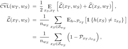
Definition 1 (Circular validation loss, CVL). Let

Sw be the set containing all the tokens of type wthroughout the whole training corpus, and call it the sample of w. Given a bilingual word pair (wT, wS)wherewT is in target languageT while wS in sourceS, letSwT andSwS be the samples for the two types respectively, andnwT and nwS the sizes of them. The empirical circular valida-tion score(CVL)d is defined as

d

CVL(wT, wS) = 1 2xSE,xT

[ b

L(xT, wS) +Lb(xS, wT) ]

,

b

L(xT, wS) = 1 nwS

∑

xS∈S_wS Eh∼PxT

[

1{h(xS)̸=zxS} ]

= 1

nw_S ∑

xS∈S_wS (

1− PxT,z_xS )

,

where PxT,k is the conditional probability of to-kenxT assigned with topick. Taking expectations

over all tokensxS andxT, we have generalCVL:

CVL(wT, wS) = 1 2xSE,xT

[L(xT, wS) +L(xS, wT)],

L(xT, wS) = ExSEh∼PxT

[

1{h(xS)̸=zxS}

] .

When sampling a tokenxT, we still follow the two-step process as in Equation (2), but instead of labeling xT itself, we use its conditional PxT to label the entire sample of a word type wS in the source language. Since all the topic labels for the source language are fixed, we take them as the as-sumed “correct” labelings, and compare xS’s la-bels and the predictions fromPxT. This is the in-tuition behindCVL.

Note that the choice of word typeswT andwSto calculate CVLd is arbitrary. However, CVLd is only meaningful when the two word types are seman-tically related, such as word translations, because those word pairs are where the knowledge trans-fer takes place. On the other hand, the Gibbs sam-pler does not calculate thisCVLdexplicitly, and thus adding reverse validation step does not affect the training of the model. It does, however, help us to expose and analyze the knowledge transfer mech-anism. In fact, as we show in the next theorem, sampling is also a procedure of optimizingCVL.d

Theorem 1. Let CVLd(t)(wT, wS) be the

empiri-cal circular validation loss of any bilingual word pair at iteration t of Gibbs sampling. Then

d

Proof. See Appendix. 2.3 PAC-Bayes View

A question following the formulation of CVLd is, what factors could lead to better transfer during this process, particularly for semantically related words? To answer this, we turn to theory that bounds the performance of classifiers and apply this theory to this formulation of topic sampling as classification.

The PAC-Bayes theorem was introduced by

McAllester (1999) to bound the performance of Bayes classifiers. Given a hypothesis set H, the majority vote classifier (or Bayes classifier) uses every hypothesis h ∈ H to perform binary clas-sification on an examplex, and uses the majority output as the final prediction. Since minimizing the error by Bayes classifier is NP-hard, an alter-native way is to use aGibbs classifieras approxi-mation. The Gibbs classifier first draws a hypoth-esish ∈ Haccording to a posterior distribution over H, and then uses this hypothesis to predict the label of an examplex(Germain et al.,2012). The generalization loss of this Gibbs classifier can be bounded as follows.

Theorem 2 (PAC-Bayes theorem, McAllester

(1999)). LetP be a posterior distribution over all classifiersh∈ H, andQa prior distribution. With a probability at least1−δ, we have

L ≤ Lb+

√

1 2n

(

KL (P||Q) + ln2

√

n δ

)

,

whereLandLbare the general loss and the empir-ical loss on a sample of sizen.

In our framework, a tokenxT provides a poste-riorPxT overK classifiers. The lossLb(xT, wS) is then calculated on a sample ofSwS in language

S. The following theorem shows that for a bilin-gual word pair(wT, wS), the generalCVLcan be bounded with several quantities.

Theorem 3. Given a bilingual word pair (wT, wS), with probability at least1−δ, the

fol-lowing bound holds:

CVL(wT, wS) ≤ CVLd(wT, wS) + (3)

1 2

√

1

n

(

KLwT + KLwS+ 2 ln 2

δ

)

+lnn

⋆

n ,

n= min{nwT, nwS

}

, n⋆ = max{nwT, nwS

}

.

For brevity we use KLw to denote KL(Px||Qx),

where Px is the conditional distribution from

Gibbs sampling of tokenxwith word type wthat gives highest lossLb(x, w), andQxa prior.

Proof. See Appendix. 2.4 Multilevel Transfer

Recall that knowledge transfer happens through priors in topic models (Section2.1). Because the KL-divergence terms in Theorem 3 include this prior Q, we can use this theorem to analyze the transfer mechanisms more concretely.

The conditional distribution for sampling a topiczxfor a tokenxduring sampling can be fac-torized into document-topic and topic-word levels:

Px,k = Pr (zx=k|wx=w,w−,z−)

= Pr (zx=k|z−)·Pr (wx=w|zx=k,w−,z−) ∝ Pr (zx=k|z−)

| {z }

document level

·Pr (zx=k|wx=w,w−)

| {z }

word level

∆

= Pθ,x,k· Pφ,x,k,

Px

∆

= Pθ,x⊗ Pφ,x,

where⊗is element-wise multiplication. Thus, we have the following inequality:

KL (Px||Qx) = KL (Pθ,x⊗ Pφ,x||Qθ,x⊗Qφ,x)

≤ KL (Pθ,x||Qθ,x) + KL (Pφ,x||Qφ,x),

and the KL-divergence term in Theorem3is sim-ply the sum of the KL-divergences between the conditional and prior distributions on all levels.

Recall that PLTM transfers knowledge at the document level, through Qθ,x, by linking docu-ment translations together (Equation (1)). Assume the current token x is from a target document linked to a document dS in the source language. Then the prior forPθ,x isθb(dS),i.e., the normal-ized empirical distribution over topics ofdS.

Since the words are generatedwithineach lan-guage underPLTM,i.e.,ϕ(_kS)is irrelevant toϕ(_kT), no transfer happens at the word level. In this case, Qφ,x, the prior for Pφ,x, is simply a K -dimensional uniform distributionU. Then:

KLw ≤ KL

(

Pθ,x||bθ(dS)

)

+ KL (Pφ,x||U)

= KL

(

Pθ,x||θb(dS)

)

| {z }

crosslingual entropy

+ logK−H(Pφ,x)

| {z }

monolingual entropy .

Most multilingual topic models are generative admixture models in which the conditional proba-bilities can be factorized into different levels, thus KL-divergence term in Theorem3can be decom-posed and analyzed in the same way as in this section for models that have transfer at other lev-els, such asHao and Paul (2018),Heyman et al.

(2016), and Hu et al. (2014). For example, if a model has word-level transfer, i.e.,the model as-sumes that word translations share the same distri-butions, we have a KL-divergence term as,

KLw ≤ KL

(

Pφ,x||φb(wS)

)

+ KL(Pθ,x||U)

= KL

(

Pφ,x||φb(wS)

)

+ logK−H(Pθ,x),

wherewSis the word translation to wordw.

3 Off-Site Transfer

Off-site transfer refers to language transfer that happens while applying trained topic models to downstream crosslingual tasks such as document classification. Because transfer happens using the trained representations, the performance of off-site transfer heavily depends on that of on-off-site transfer. To analyze this problem, we focus on the task of crosslingual document classification.

In crosslingual document classification, a doc-ument classifier,h, is trained on documents from one language, andhis then applied to documents from another language. Specifically, after training bilingual topic models, we haveK bilingual word distributions {ϕb(_kS)}K_k=1 and {ϕb(_kT)}K_k=1. These two distributions are used to infer document-topic distributions bθ on unseen documents in the test corpus, and each document is represented by the inferred distributions. A document classifier is then trained on theθbvectors as features in source languageSand tested on the targetT.

We aim to show how the generalization risk on target languagesT, denoted asRT(h), is related to the training risk on source languagesS,RcS(h). To differentiate the loss and classifiers in this section from those in Section 2, we use the term “risk” here, andh refers to the document classifiers, not the topic labeling process by the sampler.

3.1 Languages as Domains

Classic learning theory requires training and test sets to come from the same distribution D, i.e., (θ, y) ∼ D, whereθ is the document representa-tion (features) andythe document label (Valiant,

1984). In practice, however, corpora in S and

T may be sampled from different distributions, i.e., D(S) = {(θb(dS), y)} ∼ Db(S) and D(T) =

{(θb(dT)_{, y)}} ∼ Db(T)_{. We refer to these} distribu-tions as document spaces. To relate RT(h) and

c

RS(h), therefore, we have to take their distribu-tion bias into consideradistribu-tion. This is often formu-lated as a problem of domain adaptation, and here we can formulate this such that each language is treated as a “domain”.

We follow the seminal work byBen-David et al.

(2006), and defineH-distance as follows.

Definition 2 (H-distance, Ben-David et al.

(2006)). LetHbe a symmetric hypothesis space, i.e., for every hypothesis h ∈ H there exists its counterpart 1−h ∈ H. We let m = D(S) +

D(T), the total size of test corpus. The H -distance betweenDb(S)andDb(T)is defined as

1 2dbH

( b

D(S)_,Db(T))

= max

h∈H

1

m

∑

ℓ∈{S,T}

∑

xd:h(xd)=ℓ

1{xd∈D(ℓ)

}

,

wherexdis the representation for documentd, and h(xd)outputs the language of this document.

This distance measures how identifiable the lan-guages are based on their representations. If source and target languages are from entirely dif-ferent distributions, a classifier can easily identify language-specific features, which could affect per-formance of the document classifiers.

With H-distances, we have a measure of the “distance” between the two distributionsDb(S)and

b

D(T)_{. We state the following theorem from} do-main adaptation theory.

Theorem 4 (Ben-David et al. (2006)). Let m be the corpus size of the source language, i.e.,m =

D(S)_{, c the VC-dimension of document} classi-fiersh∈ H, anddb_H

( b

D(S)_,Db(T))_{theH-distance} between two languages in the document space. With probability at least 1−δ, we have the fol-lowing bound,

RT(h) ≤ RbS(h) +dbH

( b

D(S)_,Db(T))₊b_λ+

√

4

m

(

clog2em

c + log

4

δ

)

, (4)

b

λ = min

h∈H

b

The term bλin Theorem 4 defines a joint risk, i.e., the training error on both source and target documents. This term usually cannot be estimated in practice since the labels for target documents are unavailable. However, we can still calculate this term for the purpose of analysis.

The theorem shows that the crosslingual clas-sification risk is bounded by two critical compo-nents: the H-distance, and the joint risk bλ. In-terestingly, these two quantities are based on the same set of features with different labeling rules: for H-distance, the label for each instance is its language, whileλbuses the actual document label. Therefore, a better bound requires the consistency of features across languages, both in language and document labelings.

3.2 From Words to Documents

Since consistency of features depends on the doc-ument representationsθb, we need to trace back to the upstream training of topic models and show how the errors propagate to the formation of doc-ument representations. Thus, we first show the re-lations between CVLd and word representations φb in the following lemma.

Lemma 1. Given any bilingual word pair (wT, wS), let φb(w) denote the distribution over

topics of word typew. Then we have,

1−φb(wT)⊤·_φb(wS) ≤ d

CVL(wT, wS).

Proof. See Appendix.

We need to connect the word representationsφb, which are central to on-site transfer, to the docu-ment representations θb, which are central to off-site transfer. To do this, we make an assumption that the inferred distribution over topics θb(d) for each test document dis a weighted average over all word vectors,i.e.,θb(d)∝∑_wf_wd·φb(w), where

fd

wis the normalized frequency of wordwin docu-mentd(Arora et al.,2013). When this assumption holds, we can bound the similarity of document representations θb(dS) _{and θ}b(dT) _{in terms of word} representations and hence theirCVL.d

Theorem 5. Let θb(dS) _{be the distribution over} topics for document dS (similarly for dT), F(dS, dT) =

(∑

wSf

dS

wS 2

·∑wT f

dT

wT 2)12

where

f_wd is thenormalizedfrequency of wordwin doc-umentd, andK the number of topics. Then

b

θ(dS)⊤·θb(dT)

≤ F(dS, dT)·

√

K· ∑

wS,wT

(_d

CVL(wT, wS)−1

)2

.

Proof. See Appendix.

This provides a spatial connection between doc-ument pairs and word pairs they have. Many ker-nalized classifiers such as support vector machines (SVM) explicitly use this inner product in the dual optimization objective (Platt,1998). Since the in-ner product is directly related to the cosine simi-larity, Theorem5indicates that if two documents are spatially close, their inner product should be large, and thus the CVLd of all word pairs they share should be small. In an extreme case, if

d

CVL(wT, wS) = 1 for all the bilingual word pairs appearing in document pair (dS, dT), then

b

θ(dS)⊤ _·θb(dT) _{= 0, meaning the two documents} are orthogonal and tend to be irrelevant topically.

With upstream training discussed in Section2, we see thatCVLd has an impact on the consistency of features across languages. A lowCVLd indicates that the transfer from source to target is sufficient in two ways. First, languages share similar distri-butions, and therefore, it is harder to distinguish languages based on their distributions. Second, if there exists a latent mapping from a distribution to a label, it should produce similar labeling on both source and target data since they are similar. These two aspects correspond to the languageH -distance and joint riskbλin Theorem4.

4 Experiments

We experiment with five languages: Arabic (AR, Semitic), German (DE, Germanic), Spanish (ES, Romance), Russian (RU, Slavic), and Chinese (ZH, Sinitic). In the first two experiments, we pair each with English (EN, Germanic) and train PLTM on each language pair individually.

Training Data For each language pair, we use a subsample of3,000Wikipedia comparable doc-uments, i.e., 6,000 documents in total. We set

K = 50, and trainPLTMwith default hyperparam-eters (McCallum,2002). We run each experiment five times and average the results.

as the document label. In our classification exper-iments, we useculture,technology, andeducation as the labels to perform multiclass classification.

Evaluation To evaluate topic qualities, we use Crosslingual Normalized Pointwise Mutual Infor-mation (Hao et al.,2018,CNPMI), an intrinsic met-ric of crosslingual topic coherence. For any bilin-gual word pair(wT, wS),

CNPMI(wT, wS) = −

log Pr(wT,wS) Pr(wT) Pr(wS) log Pr (wT, wS)

, (6)

where Pr (wT, wS) is the occurrence of wT and wS appearing in the same pair of comparable documents. We use 10,000 Wikipedia compa-rable document pairs outside PLTM training data for each language pair to calculateCNPMIscores. All datasets are publicly available at http://

opus.nlpl.eu/ (Tiedemann, 2012).

Addi-tional details of our datasets and experiment setup can be found in the appendix.

4.1 Sampling as Circular Validation

Our first experiment shows howCVLd changes over time during Gibbs sampling. According to the definition, the arguments of CVLd can include any bilingual word pairs; however, we suggest that it should be calculated specifically among word pairs that are expected to be related (and thus en-able transfer). In our experiments, we select word pairs in the following way.

Recall that the output of a bilingual topic model is K topics, where each language has its own distribution. For each topic k, we can calculate

d

CVL(wS, wT)such thatwS andwT belong to the same topic (i.e., are in the top C most probable words in that topic), from the two languages, re-spectively. Using a cardinalityC for each of the

Ktopics, we have in totalC2×Kbilingual word pairs in the calculation ofCVL.d

At certain iterations, we collect the topic words as described above with cardinality C = 5, and calculateCVLd(wT, wS),CNPMI(wT, wS), and the error term (the1₂√· · ·term in Theorem3) of all the bilingual word pairs. In the middle panel of Fig-ure 2, CVLd over all word pairs from topic words is decreasing as sampling proceeds and becomes stable by the end of sampling. On the other hand, the correlations betweenCNPMIandCVLd are con-stantly decreasing. The negative correlations be-tween CVLd andCNPMI implies that lowerCVLd is

associated with higher topic quality, since higher-quality topic has higherCNPMIbut lowerCVL.d

4.2 What the PAC-Bayes Bound Shows

Theorem3provides insights into how knowledge is transferred during sampling and the factors that could affect this process. We analyze this bound from two aspects, the size of the training data (cor-responding to ln_nn⋆ term) and model assumptions (as in the crosslingual entropy terms).

4.2.1 Training Data: Downsampling

One factor that could affect CVL, according tod Theorem3, is the balance of tokens of a word pair. In an extreme case, if a word type wS has only one token, while another word typewT has a large number of tokens, the transfer fromwS towT is negligible. In this experiment, we will test if in-creasing the ratio term ln_nn⋆ in the corpus lowers the performance of crosslingual transfer learning.

To this end, we specify a sample rate ρ = 0.2,0.4,0.6,0.8, and 1.0. For each word pair (wT, wS), we calculate n as in the ratio term

lnn⋆

n , and remove (1− ρ) · n tokens from the corpus (rounded to the nearest integer). Smaller

ρ removes more tokens from the corpus and thus yields a larger ratio term on average.

We use a dictionary from Wiktionary to col-lect word pairs, where each word pair (wS, wT) is a translation pair. Figure3shows the results of downsampling using these two methods. Decreas-ing the sample rate ρ lowers the topic qualities. This implies that althoughPLTMcan process com-parable corpora, which need not be exact transla-tions, one still needs to be careful about the token balance between linked document pairs.

For many low-resource languages, the target language corpus is much smaller than the source corpus, so the effect of this imbalance is important to be aware of. This is an important issue when choosing comparable documents, and Wikipedia is an illustrative example. Although one can col-lect comparable documents via Wikipedia’s inter-language links, articles under the same title but in different languages can have very large varia-tions on document length, causing the imbalance of samples ln_nn⋆, and thus potentially suboptimal performance of crosslingual training.

4.2.2 Model Assumptions

1 _{10 20 40 60 80 100 500} 1000 Iterations

0.50 0.60 0.70 0.80 0.90

dcvl ( wT ,w S )

1 _{10 20 40 60}

80 100 500 ₁₀₀₀

Iterations 0.50

0.40 0.30 0.20 0.10 0.00

C orrelations ( cnpmi , dcvl )

1 _{10 20 40 60 80 100 500} 1000 Iterations 0.19 0.20 0.21 0.22 0.23 0.24 0.25 Erro r term

0.2 0.4 0.6 0.8 1.0

Sample rate⇢ 0.12

0.14 0.16 0.18 0.20 0.22 0.24

C

NPMI

AR DE ES RU ZH

1 _{10 20 40 60 80 100 500} 1000

Iterations 0.50

0.60 0.70 0.80 0.90

dcvl ( wT ,w S )

1 _{10 20 40 60 80 100 500} 1000

Iterations 0.50

0.60 0.70 0.80 0.90

dcvl ( wT ,w S )

1 _{10 20 40 60 80 100 500} 1000

Iterations 0.50

0.60 0.70 0.80 0.90

dcvl ( wT ,w S )

Figure 2: As Gibbs sampling progresses,CVLdof topic words drops, which leads to higher quality topics, and thus increasesCNPMI. The left panel shows this negative correlation, and we use shades to indicate standard deviations across five chains.

0.2 0.4 0.6 0.8 1.0

Sample rate⇢

0.12 0.14 0.16 0.18 0.20 0.22 0.24

cnpmi

0.2 0.4 0.6 0.8 1.0

Sample rate⇢

0.12 0.14 0.16 0.18 0.20 0.22 0.24

cnpmi

0.2 0.4 0.6 0.8 1.0

Sample rate⇢

0.12 0.14 0.16 0.18 0.20 0.22 0.24

C

NPMI

AR DE ES RU ZH

C = 5 C = 10

cnp m i ( wT ,w S )

Figure 3: Increasing ρ results in smaller values of

lnn⋆

n for translation pairs. Topic quality, evaluated by CNPMI, increases as well.

level and word level, and we prefer a model with low crosslingual entropy but high monolingual en-tropy. In this experiment, we show how these two quantities affect the topic qualities, using English-German (EN-DE) documents as an example.

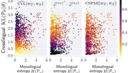
GivenPLTMoutput in (EN,DE) and a cardinality

C= 5, we collectC2×Kbilingual word pairs as described in Section4.1. For each word pair, we calculate three quantities: CVL,d CNPMI, and the inner product of the word representations. In Fig-ure4, each dot is a word pair(wS, wT)colored by the values of these quantities. The word pair dots are positioned by their crosslingual and monolin-gual entropies.

We observe that CVLd decreases with crosslin-gual entropy on document level. The larger the crosslingual entropy, the harder it is to get a low

d

CVL because it needs larger monolingual entropy to decrease the bound, as shown in Section 2.4. On the other hand, the inner product of word pairs shows an opposite pattern of CVL, indicating ad negative correlation (Lemma 1). In Figure 2 we

0 2 4 6

0.0 0.5 1.0 1.5 2.0 2.5 3.0 3.5 4.0

0.2 0.4 0.6 0.8

0 2 4 6

0.0 0.5 1.0 1.5 2.0 2.5 3.0 3.5 4.0

0.2 0.4 0.6 0.8

0 2 4 6

0.0 0.5 1.0 1.5 2.0 2.5 3.0 3.5 4.0

0.0

0.2

0.4

0.6

0.8

Crosslingual K L( P✓ || ✓

) cvl(wTd , wS) '_b(wT)>_·'b(wS) cnpmi(wT, wS)

0 2 4

6 .0 0

0 .5 1 .0 1 .5 2 .0 2 .5 3 .0 3 .5 4 .0 0 . 2 0 . 4 0 . 6 0 . 8 0.8 0.4 0.2 0.6 Monolingual

H(P')

entropy entropyMonolingualH(P')

Monolingual

H(P') entropy

Figure 4: Each dot is a (EN,DE) word pair, and its color shows corresponding values of the indicated quantity. Best viewed in color.

see the correlation between CNPMI and CVLd is around −0.4 at the end of sampling, so there are fewer clear patterns forCNPMIin Figure4. How-ever, we also notice that the word pairs with higher CNPMI scores often appear at the bottom where crosslingual entropy is low while the monolingual entropy is high.

4.3 Downstream Task

We move on to crosslingual document classifica-tion as a downstream task. At various iteraclassifica-tions of Gibbs sampling, we infer topics on the test sets for another500iterations and calculate the quan-tities shown in the Figure5(averaged over all lan-guages), including theH-distances for both train-ing and test sets, and the joint riskbλ.

We treat English as the source language and train support vector machines to obtain the best classifierh⋆ that fits the English documents. This classifier is then used to calculate the source and target risksRbS(h⋆)andRbT(h⋆). We also include

1

rep-1 _{10 20 40 60 80 100 500} 1000

Iterations

0.50

0.60

0.70

0.80

0.90

Distances

1 _{10 20 40 60 80 100 500} 1000 Iterations

0.50

0.60

0.70

0.80

0.90

Distances

1 _{10 20 40 60 80 100 500}

1000 Iterations

0.50 0.60 0.70 0.80 0.90

Distances

1 _{10 20 40 60 80 100 500}

1000 Iterations

0.50

0.60

0.70

0.80

0.90

Distances

1 10 20 40 60 80 100 500 1000 Iterations

0.40 0.50 0.60

b

RT(h?) RbS(h?) b train 1

2dbH

⇣ b

D(S)_,Db(T)⌘ _test1

2dbH

⇣ b

D(S)_,Db(T)⌘ 1

2dbH(S, T)

1 _{10 20 40 60 80 100 500} 1000 Iterations

0.40 0.50 0.60 0.70 0.80

C

lassification

risks

1 _{10 20 40 60 80 100 500} 1000

Iterations

0.40 0.50 0.60 0.70 0.80

Distances

1 _{10 20 40 60 80 100 500} 1000

Iterations 0.50

0.60 0.70 0.80 0.90

Distances

1 _{10 20 40 60 80 100 500} 1000

Iterations

0.40 0.50 0.60 0.70 0.80

C

lassification

risks

1 _{10 20 40 60 80 100 500} 1000

Iterations 0.40

0.50 0.60 0.70 0.80

C

lassification

risks

1 _{10 20 40 60 80 100 500} 1000 Iterations

0.40 0.50 0.60 0.70 0.80

C

lassification

risks

AR DE ES RU ZH

1

10 20 40 60 80 100 500₁₀₀₀

Iterations 0.50

0.60 0.70 0.80 0.90

Distances

1

10 20 40 60 80 100 500₁₀₀₀

Iterations 0.50

0.60 0.70 0.80 0.90

Distances

1

10 20 40 60 80 100 500₁₀₀₀

Iterations 0.50

0.60 0.70 0.80 0.90

Distances

1

10 20 40 60 80 100 500₁₀₀₀

Iterations 0.50

0.60 0.70 0.80 0.90

Distances

1

10 20 40 60 80 100 500₁₀₀₀

Iterations 0.50

0.60 0.70 0.80 0.90

Distances

Figure 5: Gibbs sampling optimizesCVLd, which decreases the joint riskλbandH-distances for test data.

resentations φb. As mentioned in Section 3.1, we train support vector machines to use languages as labels, and the accuracy score as theH-distance.

The classification risks, such as RbS(h⋆),

b

RT(h⋆), andbλ, are decreasing as expected (upper row in Figure5), which shows very similar trends asCVLd in Figure2. On the other hand, we notice that the H-distances of training documents and vocabularies, 1₂db_H

( b

D(S)_,Db(T))_and 1

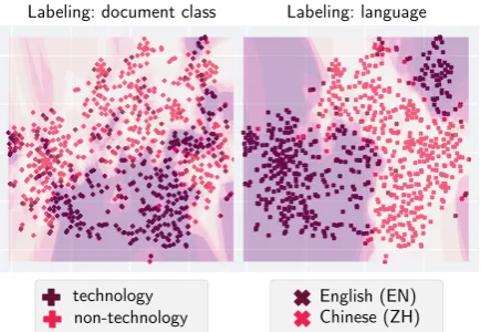
2dbH(S, T), stabilize around0.5to0.6, meaning it is difficult to differentiate the languages based on their rep-resentations. Interestingly, theH-distances of test documents are at a less ideal value, although they are slightly decreasing in most of the languages exceptAR. However, recall that the target risk also depends on other factors thanH-distance (Theo-rem4), and we use Figure6to illustrate this point. We further explore the relationship between the predictability of languages vs document classes in Figure6. We collect documents correctly classi-fied for both document class and language labels, from which we randomly choose200documents for each language, and useθbto plot t-SNE scatter-plots. Note that the two plots are from the same set of documents, and so the spatial relations be-tween any two points are fixed, but we color them with different labelings. Although the classifier can identify the languages (right panel), the fea-tures are still consistent, because on the left panel, the decision boundary changes its direction and also successfully classifies the documents based on actual label class. This illustrates why a single

H-distance does not necessarily mean inconsistent features across languages and high target risks.

Labeling: document class Labeling: language

English (EN) Chinese (ZH) technology

non-technology

Figure 6: Although the classifier identifies the lan-guages (right), the features are still consistent based on actual document class (left).

5 Conclusions and Future Directions

This study gives new insights into crosslingual transfer learning in multilingual topic models. By formulating the inference process as a circular val-idation, we derive a PAC-Bayesian theorem to show the factors that affect the success of crosslin-gual learning. We also connect topic model learn-ing with downstream crossllearn-ingual tasks to show how errors propagate.

References

Sanjeev Arora, Rong Ge, Yonatan Halpern, David M. Mimno, Ankur Moitra, David Sontag, Yichen Wu, and Michael Zhu. 2013. A Practical Algorithm for

Topic Modeling with Provable Guarantees. In

Pro-ceedings of the 30th International Conference on Machine Learning, ICML 2013, Atlanta, GA, USA, 16-21 June 2013, pages 280–288.

Maria Barrett, Frank Keller, and Anders Søgaard. 2016.

Cross-lingual Transfer of Correlations between Parts

of Speech and Gaze Features. InCOLING 2016,

26th International Conference on Computational Linguistics, Proceedings of the Conference: Tech-nical Papers, December 11-16, 2016, Osaka, Japan, pages 1330–1339.

Shai Ben-David, John Blitzer, Koby Crammer, and Fernando Pereira. 2006. Analysis of

Representa-tions for Domain Adaptation. InAdvances in

Neu-ral Information Processing Systems 19, Proceedings of the Twentieth Annual Conference on Neural In-formation Processing Systems, Vancouver, British Columbia, Canada, December 4-7, 2006, pages 137–144.

David M. Blei, Andrew Y. Ng, and Michael I. Jordan. 2003. Latent Dirichlet Allocation. Journal of Ma-chine Learning Research, 3:993–1022.

Lorenzo Bruzzone and Mattia Marconcini. 2010. Do-main Adaptation Problems: A DASVM

Classifica-tion Technique and a Circular ValidaClassifica-tion Strategy.

IEEE Transactions on Pattern Analysis and Machine Intelligence, 32(5):770–787.

Manaal Faruqui and Chris Dyer. 2014. Improving Vec-tor Space Word Representations Using Multilingual

Correlation. In Proceedings of the 14th

Confer-ence of the European Chapter of the Association for Computational Linguistics, EACL 2014, April 26-30, 2014, Gothenburg, Sweden, pages 462–471.

Pascal Germain, Amaury Habrard, Franc¸ois Laviolette, and Emilie Morvant. 2012. PAC-Bayesian Learning

and Domain Adaptation.CoRR, abs/1212.2340.

Thomas L Griffiths and Mark Steyvers. 2004. Find-ing Scientific Topics. Proceedings of the National academy of Sciences, 101(suppl 1):5228–5235.

E. Dario Guti´errez, Ekaterina Shutova, Patricia Licht-enstein, Gerard de Melo, and Luca Gilardi. 2016.

Detecting Cross-cultural Differences Using a

Multi-lingual Topic Model. Transactions of the

Associa-tion for ComputaAssocia-tional Linguistics, 4:47–60.

Shudong Hao, Jordan L. Boyd-Graber, and Michael J. Paul. 2018. Lessons from the Bible on Modern Topics: Low-Resource Multilingual Topic Model

Evaluation. In Proceedings of the 2018

Confer-ence of the North American Chapter of the Associ-ation for ComputAssoci-ational Linguistics: Human Lan-guage Technologies, NAACL-HLT 2018, New Or-leans, Louisiana, USA, June 1-6, 2018, Volume 1 (Long Papers), pages 1090–1100.

Shudong Hao and Michael J. Paul. 2018. Learning

Multilingual Topics from Incomparable Corpora. In

Proceedings of the 27th International Conference on Computational Linguistics, COLING 2018, Santa Fe, New Mexico, USA, August 20-26, 2018, pages 2595–2609.

Geert Heyman, Ivan Vulic, and Marie-Francine Moens. 2016. C-BiLDA: Extracting Cross-lingual Topics from Non-parallel Texts by Distinguishing Shared

from Unshared Content. Data Mining and

Knowl-edge Discovery, 30(5):1299–1323.

Yuening Hu, Jordan L. Boyd-Graber, Brianna Satinoff, and Alison Smith. 2014. Interactive Topic Model-ing.Machine Learning, 95(3):423–469.

Jagadeesh Jagarlamudi and Hal Daum´e III. 2010. Ex-tracting Multilingual Topics from Unaligned

Com-parable Corpora. In Advances in Information

Re-trieval, 32nd European Conference on IR Research, ECIR 2010, Milton Keynes, UK, March 28-31, 2010. Proceedings, pages 444–456.

Alexandre Klementiev, Ivan Titov, and Binod Bhat-tarai. 2012. Inducing Crosslingual Distributed

Rep-resentations of Words. InCOLING 2012, 24th

In-ternational Conference on Computational Linguis-tics, Proceedings of the Conference: Technical Pa-pers, 8-15 December 2012, Mumbai, India, pages 1459–1474.

Tengfei Ma and Tetsuya Nasukawa. 2017. Inverted Bilingual Topic Models for Lexicon Extraction from

Non-parallel Data. InProceedings of the

Twenty-Sixth International Joint Conference on Artificial In-telligence, IJCAI 2017, Melbourne, Australia, Au-gust 19-25, 2017, pages 4075–4081.

David A. McAllester. 1999. PAC-Bayesian Model

Av-eraging. InProceedings of the Twelfth Annual

Con-ference on Computational Learning Theory, COLT 1999, Santa Cruz, CA, USA, July 7-9, 1999, pages 164–170.

Andrew Kachites McCallum. 2002. MALLET: A

Ma-chine Learning for Language Toolkit.

David M. Mimno, Hanna M. Wallach, Jason Narad-owsky, David A. Smith, and Andrew McCallum. 2009. Polylingual Topic Models. InProceedings of the 2009 Conference on Empirical Methods in Natu-ral Language Processing, EMNLP 2009, 6-7 August 2009, Singapore, A meeting of SIGDAT, a Special Interest Group of the ACL, pages 880–889.

Xiaochuan Ni, Jian-Tao Sun, Jian Hu, and Zheng Chen. 2009. Mining Multilingual Topics from Wikipedia. InProceedings of the 18th International Conference on World Wide Web, WWW 2009, Madrid, Spain, April 20-24, 2009, pages 1155–1156.

John Platt. 1998. Sequential minimal optimization: A

fast algorithm for training support vector machines.

Sebastian Ruder, Ivan Vuli´c, and Anders Søgaard. 2018. A Survey of Cross-lingual Word Embedding

Models. Journal of Artificial Intelligence Research,

abs/1706.04902.

Ekaterina Shutova, Lin Sun, E. Dario Guti´errez, Patri-cia Lichtenstein, and Srini Narayanan. 2017. Mul-tilingual Metaphor Processing: Experiments with

Semi-Supervised and Unsupervised Learning.

Com-putational Linguistics, 43(1):71–123.

Wim De Smet and Marie-Francine Moens. 2009.

Cross-language Linking of News Stories on the Web

Using Interlingual Topic Modelling. InProceedings

of the 2nd ACM Workshop on Social Web Search and Mining, CIKM-SWSM 2009, Hong Kong, China, November 2, 2009, pages 57–64.

J¨org Tiedemann. 2012. Parallel Data, Tools and

Inter-faces in OPUS. In Proceedings of the Eighth

In-ternational Conference on Language Resources and Evaluation, LREC 2012, Istanbul, Turkey, May 23-25, 2012, pages 2214–2218.

Leslie G. Valiant. 1984. A Theory of the Learnable.

Communications of the ACM, 27(11):1134–1142.

Erheng Zhong, Wei Fan, Qiang Yang, Olivier Ver-scheure, and Jiangtao Ren. 2010. Cross Valida-tion Framework to Choose amongst Models and

Datasets for Transfer Learning. InMachine

Learn-ing and Knowledge Discovery in Databases, Euro-pean Conference, ECML PKDD 2010, Barcelona, Spain, September 20-24, 2010, Proceedings, Part III, pages 547–562.

Appendix A Notation

See Table1.

Appendix B Proofs

Theorem 1. Let CVLd(t)(wT, wS) be the

empiri-cal circular validation loss of any bilingual word pair at iteration t of Gibbs sampling. Then

d

CVL(t)(wT, wS)converges ast→ ∞.

Proof. We first notice the triangle inequality:

dCVL(t)(wT, wS)−CVLd(t−1)(wT, wS)

= _E

xS,xT [

b

L(t)

(xT, wS) +Lb(t)(xS, wT) ]

− E

xS,xT [

b

L(t−1)

(xT, wS) +Lb(t−1)(xS, wT) ]

= xT∈SEwT

[ b

L(t)

(xT, wS) ]

+ E

xS∈SwS [

b

L(t)

(xS, wT) ]

− E

xT∈SwT [

b

L(t−1)

(xT, wS) ]

− E

xS∈SwS [

b

L(t−1)

(xS, wT)]

Notation Description

S,T Source and target languages. They are interchangeable during Gibbs sampling. For example, when training English and German, English can be either source or target.

wℓ Aword typeof languageℓ. xℓ An individualtokenof languageℓ. zxℓ The topic assignment of tokenxℓ.

Swℓ The sample of word typewℓ, the set con-taining all the tokensxℓ that are of this word type.

Pxℓ,Pxℓ,k Pxℓ denotes the conditional distribution over all topics for tokenxℓ. The condi-tional probability of sampling a topick

fromPxℓis denoted asPxℓ,k.

D(ℓ) The set of documents in language ℓ. This usually refers to the test corpus.

b

D(ℓ) _{The array of document representations} from the corpus D(ℓ) and their docu-ment labels.

b

ϕ(_kℓ) The empirical distribution over vocab-ulary of language ℓ for topic k = 1, . . . , K.

b

φ(w) The word representation, i.e., the em-pirical distribution over K topics for a word type w. This can be obtained by re-normalizingϕb(_kℓ).

b

θ(d) The document representation, i.e., the empirical distribution overK topics for a documentd.

Table 1: Notation table.

≤ E

xT∈SwT [

b

L(t)

(xT, wS) ]

− E

xT∈SwT [

b

L(t−1)

(xT, wS) ]

+ _E

xS∈SwS [

b

L(t)

(xS, wT) ]

− E

xS∈SwS [

b

L(t−1)

(xS, wT)]

≡ ∆ _E

xT∈SwT [

b

L(xT, wS) ]

+ ∆ _E

xS∈SwS [

b

L(xS, wT)]

≤ ∆ E

xT∈SwT [

b

L(xT, wS)]+

∆xS∈SEwS [

b

L(xS, wT)].

We look at the first term of the last equation, and the other term can be derived in the same way. We usePxT to denote the invariant distribution of the conditionalPx(tT) ast → ∞. Additionally, let

to-kenxT being assigned to topiczxS:

PxT,zxS = Pr (k=zxS;w=wxT,z−,w−).

Another assumption we made is once the source language is converged, we keep the states of it fixed. That is,z(xtS) = z

(t−1)

xS , and only sample the target language. Taking the difference between the expectation at iterationstandt−1, we have

lim

t→∞

∆xT∈SEwT [

b

L(xT, wS)]

= lim

t→∞

xT∈SEwT

[ b

L(t)

(xT, wS) ]

− E

xT∈SwT [

b

L(t−1)

(xT, wS)]

= lim

t→∞ xET

  1

nwS ∑

xS

E_h∼P(t)

xT1 {

h(xS)̸=zx(tS) }



−E

xT   1

nw_S ∑

xS

E_h∼P(t−1)

xT 1

{

h(xS)̸=zx(tS−1) }



= lim

t→∞

1 nwS

∑

xS E

xT [

E_h∼P(t)

xT1 {

h(xS)̸=zx(tS) }

−E_h∼P(t−1)

xT 1

{

h(xS)̸=z(xtS−1) }

]

= lim

t→∞

1 nwS

∑

xS E

xT [

E_h∼P(t)

xT1{h(xS)̸=zxS}

−E_h∼P(t−1)

xT 1{h(xS)̸=zxS} ]

= lim

t→∞

1 nwS

∑

xS∈SwS

ExT∈SwT [(

1− Px(tT),zxS )

−(1− Px(tT−,z1)xS )]

= lim

t→∞

1 nwS

∑

xS∈SwS

ExT∈SwT[P

(t−1)

xT,zxS − P

(t)

xT,zxS ]

= lim

t→∞

1 nwS

∑

xS∈SwS

ExT∈SwT[PxT,zxS − PxT,zxS]

= 0.

Therefore, we have

lim

t→∞

dCVL(t)(wT, wS)−CVLd

(t−1)

(wT, wS)

≤ lim

t→∞

∆xT∈SEwT [

b

L(xT, wS)]

+

∆xS∈SEwS [

b

L(xS, wT)]

= 0.

Theorem 3. Given a bilingual word pair (wT, wS), with probability at least1−δ, the

fol-lowing bound holds:

CVL(wT, wS) ≤ CVLd(wT, wS) +

1 2

√

1

n

(

KLwT + KLwS+ 2 ln 2

δ

)

+ lnn

⋆

n ,

n= min{nwT, nwS

}

, n⋆ = max{nwT, nwS

}

.

For brevity we use KLw to denote KL(Px||Qx),

where Px is the conditional distribution from

Gibbs sampling of tokenxwith word type wthat gives highest lossLb(x, w), andQxa prior.

Proof. From Theorem 2, for target language, with probability at least1−δ,

L(xT, wS)

≤ Lb(xT, wS) + √

KL (PxT||QxT) + ln

2√n_wS

δ

2nwS

= Lb(xT, wS) + √

KL (PxT||QxT) + ln 2

δ+

lnn_wS

2n_wS

2

≡ Lb(xT, wS) +ϵ(xT, wS).

For the source language, similarly, with proba-bility at least1−δ,

L(xS, wT)

≤ Lb(xS, wT) + √

KL (PxS||QxS) + ln 2

δ +

lnn_wT

2 2nwT

≡ Lb(xS, wT) +ϵ(xS, wT).

Given a word typewT, we notice that only the KL-divergence term in ϵ(xT, wS) varies among different tokens xT. Thus, we use KLwS and KLwT to denote the maximal values of KL-divergence over all the tokens,

KLwS = KL (

Px⋆ T||Qx⋆T

) ,

x⋆T = arg max xT∈SwT

ϵ(xT, wS);

KLwT = KL (

Px⋆ S||Qx⋆S

) ,

x⋆S = arg max xS∈SwS

ϵ(xS, wT).

Let n = min{nwT, nwS}, and n

⋆ ₌

max{nwT, nwS}. Due to the fact that

√

x+√y ≤

2 √ 2

√

CVL(wT, wS)

= 1 2xSE,xT

[L(xT, wS) +L(xS, wT)]

= 1

2(ExTL(xT, wS) +ExSL(xS, wT))

≤ 1

2 (

ExT∈SwTLb(xT, wS) +ExS∈SwSLb(xS, wT) )

+1 2 (

ExT∈SwTϵ(xT, wS) +ExS∈SwSϵ(xS, wT) )

= CVLd(wT, wS)

+1 2 (

Ex_T∈SwTϵ(xT, wS) +ExS∈SwSϵ(xS, wT) )

≤ CVLd(wT, wS) +

1 2(ϵ(x

⋆

T, wS) +ϵ(x⋆S, wT))

≤ CVLd(wT, wS)

+1 2

(√ 1 2nwT

(

KLwT + ln 2 δ +

1 2lnnwT

)

+ √

1 2nwS

(

KLwS + ln 2 δ +

1 2lnnwS

))

≤ CVLd(wT, wS)

+1 2

√

KLwT + KLwS + 2 ln 2

δ

n +

(

ln (nwT ·nwS) 2n

)

≤ CVLd(wT, wS)

+1 2

√

KLw_T + KLw_S + 2 ln2_δ

n +

( lnn⋆

n )

,

which gives us the result.

Lemma 1. Given any bilingual word pair (wT, wS), let φb(w) denote the distribution over

topics of word typew. Then we have, 1−φb(wT)⊤·_φb(wS) ≤ _CVLd_(w

T, wS).

Proof. We expand the equation ofCVLd as follows,

d

CVL(wT, wS)

= 1 2xSE,xT

[ b

L(xT, wS) +Lb(xS, wT) ]

= 1 2 (

ExT [

b

L(xT, wS) ]

+ExS [

b

L(xS, wT) ])

= 1 2

( ∑ xT∈SwT

∑

xS∈SwSEh∼PxT [

1{h(xS)̸=zxS} ]

nwT ·nwS

+ ∑

x_S∈SwS ∑

x_T∈SwTEh∼PxS [

1{h(xT)̸=zxT} ]

nw_S·nw_T

)

= 1 2

( ∑ xT∈SwT

∑ xS∈SwS

(

1− PxT,zxS )

nwT ·nwS

+ ∑

xS∈SwS ∑

xT∈SwT (

1− PxS,zxT )

nwS·nwT

)

= 1−1 2

( ∑ xT∈SwT

∑

xS∈SwSPxT,zxS

nwT ·nwS

+ ∑

xS∈SwS ∑

xT∈SwT PxS,zxT

nwS·nwT

)

= 1−1 2

K ∑

k=1 (

nk|wS · ∑

xT∈SwT PxT,k

nwT ·nwS

+ nk|wT ·

∑

xS∈SwSPxS,zxT

nwS·nwT

)

= 1−1 2 K ∑ k=1 ( b φ(wS)

k · ∑

xT∈SwTPxT,k

nwT

+φb(wT)

k · ∑

x_S∈SwSPxS,zxT

nw_S

)

≥ 1−1 2 K ∑ k=1 ( b φ(wS)

k · nk|w_T

nwT

+φb(wT)

k · nk|w_S

nwS )

= 1−1 2 K ∑ k=1 ( b φ(wS)

k ·φb

(wT)

k +φb

(wT)

k ·φb

(wS)

k )

= 1−φb(wS)⊤·_φb(wT)

which concludes the proof.

Theorem 5. Let θb(dS) _{be the distribution over} topics for document dS (similarly for dT), F(dS, dT) =

(∑

wSf

dS

wS 2

·∑wT f

dT

wT 2)12

where

f_wd is thenormalizedfrequency of wordwin doc-umentd, andKthe number of topics. Then

b

θ(dS)⊤·θb(dT) ≤ F(dS, dT)

· √

K· ∑

wS,wT

( d

CVL(wT, wS)−1

)2

.

Proof. We first expand the inner product of

b

θ(dS)⊤·θb(dT)as follows,

b

θ(dS)⊤·_θb(dT)

=

K ∑

k=1 b θ(dS)

k ·bθ

(dT)

k = K ∑ k=1     ∑

wS∈V(S)

fdS

wS·φb

(wS)

k   ·   ∑

wT∈V(T)

fdT

wT ·φb

(wT)

k    

≤ F(dS, dT)· K ∑ k=1      ∑

wS∈V(S) b φ(wS)2

k   1 2 ·   ∑

wT∈V(T) b φ(wT)2

k   1 2   ,

F(dS, dT)

= 

 ∑

wS∈V(S)

fdS

wS 2   1 2 ·   ∑

wT∈V(T)

fdT

where F(dS, dT) is a constant independent of topic k, and the last inequality due to H¨older’s. We then focus on the topic-dependent part of the last inequality.

K ∑

k=1    

 ∑

wS∈V(S) b φ(wS)2

k  

1 2

·



 ∑

wT∈V(T) b φ(wT)2

k  

1 2

  

=

K ∑

k=1 

 ∑

wS,wT (

b φ(wS)

k ·φb

(wT)

k )2

 

1 2

≤ √K·  ∑K

k=1 ∑

wS,wT (

b φ(wS)

k ·φb

(wT)

k )2

 

1 2

= √K· 

 ∑

wS,wT

K ∑

k=1 (

b φ(wS)

k ·φb

(wT)

k )2

 

1 2

≤ √K· 

 ∑

wS,wT (_K

∑

k=1 b φ(wS)

k ·φb

(wT)

k )2



1 2

= √K· 

 ∑

wS,wT (

b

φ(wT)⊤·_φb(wS) )2

 

1 2

.

Thus, we have the following inequality:

b

θ(dS)⊤·θb(dT) ≤ _F(d

S, dT)·

√

K

· (

∑

wS,wT

( b

φ(wT)⊤·_φb(wS)

)2)

1 2

.

Plug in Lemma1, we see that

b

θ(dS)⊤·θb(dT) ≤ _F(d

S, dT)·

√

K

· (

∑

wS,wT

(_d

CVL(wT, wS)−1

)2

)1 2

.

Appendix C Dataset Details

C.1 Pre-processing

For all the languages, we use existing stemmers to stem words in the corpora and the entries in Wik-tionary. Since Chinese does not have stemmers, we loosely use “stem” to refer to “segment” Chi-nese sentences into words. We also use fixed stop-word lists to filter out stop stop-words. Table2lists the source of the stemmers and stopwords.

1_{http://snowball.tartarus.org;}

2

http://arabicstemmer.com; 3

https://github.com/6/stopwords-json;

4_{https://github.com/fxsjy/jieba.}

C.2 Training Sets

Our training set is a comparable corpus from Wikipedia. For each Wikipedia article page, there exists an interlingual link to view the article in another language. This interlingual link provides the same article in different languages and is com-monly used to create comparable corpora in multi-lingual studies. We show the statistics of this train-ing corpus in Table3. The numbers are calculated after stemming and lemmatization.

C.3 Test Sets

C.3.1 Topic Coherence Evaluation Sets

Topic coherence evaluation for multilingual topic models was proposed byHao et al.(2018), where a comparable corpus is used to calculate bilingual word pair co-occurrence and CNPMI scores. We use a Wikipedia corpus to calculate this score, and the statistics are shown in Table4. This Wikipedia corpus does not overlap with the training set.

C.3.2 Unseen Document Inference

We use the Global Voices (GV) corpus to create test sets, which can be retrieved from the

web-site https://globalvoices.org directly,

or from the OPUS collection athttp://opus.

nlpl.eu/GlobalVoices.php. We show the

statistics in Table 5. After the column showing number of documents, we also include the statis-tics of specific labels. The multiclass labels are mutual exclusive, and each document has only one label.

Note that although all the language pairs share the same set of English test documents, the doc-ument representations are inferred from different topic models trained specifically for that language pair. Thus, the document representations for the same English document are different across dif-ferent language pairs.

Lastly, the number of word types is based on the training set and after stemming and lemmatization. When a word type in the test set does not appear in the training set, we ignore this type.

C.3.3 Wiktionary

In downsampling experiments (Section 4.2), we use English Wiktionary to create bilin-gual dictionaries, which can be downloaded

at https://dumps.wikimedia.org/

Language Family Stemmer Stopwords

AR Semitic Assem’s Arabic Light Stemmer1 GitHub2

DE Germanic SnowBallStemmer3 NLTK

EN Germanic SnowBallStemmer NLTK

ES Romance SnowBallStemmer NLTK

RU Slavic SnowBallStemmer NLTK

ZH Sinitic Jieba4 GitHub

Table 2: List of source of stemmers and stopwords used in experiments.

English

Language #docs #token #types

AR 3,000 724,362 203,024

DE 3,000 409,381 125,071

ES 3,000 451,115 134,241

RU 3,000 480,715 142,549

ZH 3,000 480,142 141,679 Paired language Language #docs #token #types

AR 3,000 223,937 61,267

DE 3,000 285,745 125,169

ES 3,000 276,188 95,682

RU 3,000 276,462 96,568

ZH 3,000 233,773 66,275

Table 3: Statistics of the Wikipedia training corpus.

Appendix D Topic Model Configurations

For each experiment, we run five chains of Gibbs sampling using the Polylingual Topic Model im-plemented in MALLET, 5 and take the average over all chains. Each chain has1,000iterations, and we do not set a burn-in period. We set the topic numberK= 50. Other hyperparameters are

α = 50_K = 1andβ = 0.01which are the default settings. We do not enable hyperparameter opti-mization procedures.

5_{http://mallet.cs.umass.edu/}

topics-polylingual.php.

English

Language #docs #token #types

AR 10,000 3,092,721 143,504

DE 10,000 2,779,963 146,757

ES 10,000 3,021,732 149,423

RU 10,000 3,016,795 154,442

ZH 10,000 1,982,452 112,174 Paired language Language #docs #token #types

AR 10,000 1,477,312 181,734

DE 10,000 1,702,101 227,205

ES 10,000 1,737,312 142,086

RU 10,000 2,299,332 284,447

ZH 10,000 1,335,922 144,936

Table 4: Statistics of the Wikipedia corpus for topic coherence evaluation (CNPMI).

Language #docs #token #types

EN 11,012 3,838,582 104,164

AR 1,086 314,918 53,030

DE 773 334,611 38,702

ES 7,470 3,454,304 110,134

RU 1,035 454,380 67,202

ZH 1,590 804,720 61,319

#tech. #culture #edu.

EN 4,384 4,679 1,949

AR 457 430 199

DE 315 294 164

ES 2,961 3,121 1,388

RU 362 456 217

ZH 619 622 349