Torque distribution strategies for energy efficient electric vehicles with multiple drivetrains

Torque distribution strategies for energy-efficient electric

vehicles with multiple drivetrains

LENZO, Basilio <http://orcid.org/0000-0002-8520-7953>, DE FILIPPIS,

Giovanni, DIZQAH, Arash, SORNIOTTI, Aldo, GRUBER, Patrick, FALLAH,

Saber and DE NIJS, Wouter

Available from Sheffield Hallam University Research Archive (SHURA) at:

http://shura.shu.ac.uk/15643/

This document is the author deposited version. You are advised to consult the

publisher's version if you wish to cite from it.

Published version

LENZO, Basilio, DE FILIPPIS, Giovanni, DIZQAH, Arash, SORNIOTTI, Aldo,

GRUBER, Patrick, FALLAH, Saber and DE NIJS, Wouter (2017). Torque distribution

strategies for energy-efficient electric vehicles with multiple drivetrains. Journal of

Dynamic Systems, Measurement and Control, 139 (12), DS-16.

Copyright and re-use policy

See

http://shura.shu.ac.uk/information.html

Sheffield Hallam University Research Archive

Torque distribution strategies for energy-efficient electric

vehicles with multiple drivetrains

LENZO, Basilio <http://orcid.org/0000-0002-8520-7953>, DE FILIPPIS,

Giovanni, DIZQAH, Arash, SORNIOTTI, Aldo, GRUBER, Patrick, FALLAH,

Saber and DE NIJS, Wouter

Available from Sheffield Hallam University Research Archive (SHURA) at:

http://shura.shu.ac.uk/15643/

This document is the author deposited version. You are advised to consult the

publisher's version if you wish to cite from it.

Published version

LENZO, Basilio, DE FILIPPIS, Giovanni, DIZQAH, Arash, SORNIOTTI, Aldo,

GRUBER, Patrick, FALLAH, Saber and DE NIJS, Wouter (2017). Torque distribution

strategies for energy-efficient electric vehicles with multiple drivetrains. Journal of

Dynamic Systems, Measurement and Control, 139 (12), DS-16.

Repository use policy

Copyright © and Moral Rights for the papers on this site are retained by the

individual authors and/or other copyright owners. Users may download and/or print

one copy of any article(s) in SHURA to facilitate their private study or for

non-commercial research. You may not engage in further distribution of the material or

use it for any profit-making activities or any commercial gain.

Sheffield Hallam University Research Archive

American Society of

Mechanical Engineers

ASME Accepted Manuscript Repository

Institutional Repository Cover Sheet

Basillio Lenzo

First Last

ASME Paper Title: Torque distribution strategies for energy-efficient electric vehicles with multiple drivetrains

Authors:

LENZO, Basilio, DE FILIPPIS, Giovanni, DIZQAH, Arash, SORNIOTTI, Aldo, GRUBER, Patrick, FALLAH, Saber and DE NIJS, Wouter

ASME Journal Title: Journal of Dynamic Systems, Measurement and Control

Volume/Issue 139 _{Date of Publication (VOR* Online) 9th August 2017}

ASME Digital Collection URL: http://dynamicsystems.asmedigitalcollection.asme.org/article.aspx?articleid=2632222

DOI: 10.1115/1.4037003

1

Torque Distribution Strategies for Energy-Efficient

Electric Vehicles with Multiple Drivetrains

B. Lenzo1,2, G. De Filippis1, A.M. Dizqah3,1, A. Sorniotti1,*, P. Gruber1, S. Fallah1, W. De Nijs4

1

Centre for Automotive Engineering, University of Surrey, United Kingdom

2

Department of Engineering and Mathematics, Sheffield Hallam University, United Kingdom

3

Centre for Mobility and Transport, Coventry University, United Kingdom

4

Flanders MAKE, Belgium

Abstract – The paper discusses novel computationally efficient torque distribution strategies for electric vehicles with individually

controlled drivetrains, aimed at minimizing the overall power losses while providing the required level of wheel torque and yaw moment. Analytical solutions of the torque control allocation problem are derived and effects of load transfers due to driving/braking and cornering are studied and discussed in detail. Influences of different drivetrain characteristics on the front and rear axles are described. The results of an analytically-derived algorithm are contrasted with those from two other control allocation strategies, based on the off-line numerical solution of more detailed formulations of the control allocation problem (i.e., a multi-parametric non-linear programming problem). The control allocation algorithms are experimentally validated with an electric vehicle with four identical drivetrains along multiple driving cycles and in steady-state cornering. The experiments show that the computationally efficient algorithms represent a very good compromise between low energy consumption and controller complexity.

Keywords – Electric vehicle; multiple drivetrains; torque distribution; control allocation; power loss; analytical solution

1. Introduction

Electric vehicles with multiple and individually controlled drivetrains can achieve superior handling qualities through direct control of the yaw moment, also called torque-vectoring. For example, torque-vectoring can increase the maximum lateral acceleration in quasi-static conditions, and augment vehicle yaw damping during extreme transients to provide stable vehicle response. These benefits, relevant to both human-driven and self-driven electric vehicles, have extensively been discussed and experimentally demonstrated in the literature [1-4].

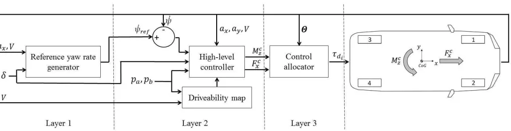
Typically, a direct yaw moment controller (see Figure 1) for an electric vehicle with multiple motors consists of three main layers: i) A reference generator (Layer 1), which determines the target values of the vehicle states (such as the reference yaw rate,

, which is calculated through a multi-dimensional look-up table in this study, see [1]) based on the driver inputs (i.e., the steering wheel angle, , and the accelerator and brake pedal positions, and ) and the measured or estimated vehicle states (e.g., vehicle speed, , and longitudinal acceleration, ). Owing to the nature of the vehicle system, in this configuration the reference generator uses feedback signals from the plant. For example, the actual yaw rate of the car is a function of and for a given . Despite the significant impact of torque-vectoring control on the cornering response, it is not possible – and would not make sense – to fully compensate for the variation of vehicle yaw response with speed and longitudinal acceleration. As a consequence, also has to be varied as a function of and , which can be estimated from vehicle sensor measurements.

ii) A high-level controller (Layer 2) generating the overall traction/braking force, , and yaw moment demands, , to achieve the reference values of the states. The yaw moment actuation is considered here through two independent drivetrains on at least one axle (i.e., torque-vectoring differentials are not considered).

iii) A low-level controller (i.e., the ‘control allocator’ in Figure 1, Layer 3), which outputs the reference torques, , for the

*_{Corresponding author. Centre for Automotive Engineering, Department of Mechanical Engineering Sciences, Faculty of Engineering and Physical Sciences (FEPS),}

University of Surrey, Guildford, GU2 7XH, United Kingdom, email: [email protected]

2

individual wheels corresponding to and computed by the high-level controller (Layer 2).

With respect to the control allocator (Layer 3), special interest is on four-wheel-drive electric vehicles because of their actuation redundancy [5-10]. For example, in straight-line conditions the overall traction/braking force demand can be generated through infinitely different front-to-rear wheel torque distributions. Moreover, in the case of four independent drivetrains (i.e., one drivetrain per wheel) infinite solutions are available for the generation of actuated through different torques at the left and right wheels. The general problem of optimally distributing the reference signals to redundant actuators is referred to as control allocation [11-13]. As mentioned before, the torque-vectoring controller can significantly alter the vehicle cornering response by controlling the yaw moment. The yaw moment is primarily generated by the difference between the sums of wheel torque values on the left- and right-hand sides of the vehicle. In this respect, the front-to-rear wheel torque distribution on each vehicle side can have an impact on the overall yaw moment, which is normally very limited. Also, the steering angle of the front wheels and the interaction between the longitudinal and lateral tire forces can induce a variation of the total yaw moment dependent on the adopted control allocation criterion. However, this influence is compensated by the feedback nature of the controller, which tends to make the vehicle follow the reference yaw rate.

For electric vehicles an important target of the control allocation algorithm is the minimization of the power losses. In particular, [2] and [5] analyze the different sources of power loss at the vehicle level, including the contributions associated with the electric motor drive, the transmission system, tire rolling resistance, and tire slip in longitudinal and lateral directions. A quasi-static model is adopted to assess the performance of different wheel torque distribution criteria. However, given the complexity of the assessed control allocation algorithms and the required state estimators, the analyses in [2] and [5] were not experimentally validated. Many papers, for instance [14-20], present advanced control allocation strategies for reducing the motor drive power losses, the tire slip power losses, or other tire-related performance indicators. They are based on relatively complex algorithms, which are quite difficult to implement in practice at the industrial level. Although the presented results show energy efficiency benefits in specific tests, the required optimal wheel torque distributions are not analyzed in detail. For real vehicle implementations, there is a clear need to better understand the physics of the system and develop simple yet effective control allocation algorithms. This objective is consistent with the general trend towards the actual implementation of optimized energy- and vehicle-related control systems [21-25].

In the specific field of electric vehicles with multiple motors, [17] derives the analytical expressions of the power loss characteristics of electric motor drives. The conclusion is that a 50:50 front-to-rear wheel torque distribution should be the most efficient solution for the case of identical drivetrains on the two axles. Nevertheless, in practice the same paper recommends to use the drivetrain/s of a single axle at low torque demands, and a 50:50 front-to-rear torque distribution at medium-high torques, without specifying the threshold for implementing the transition between the two modes. This control policy is indirectly confirmed by the experimental tests in [26] and [27], but these studies do not critically analyze the resulting optimal torque distribution. [28] presents a simple control allocation algorithm for electric vehicles with identical power loss characteristics on the front and rear axles. However, this preliminary investigation does not consider the variation of tire rolling resistance and slip ratios as a result of load transfers due to longitudinal and lateral accelerations.

This paper significantly extends the preliminary results of [28] towards the implementation of simple and industrially viable control allocation formulations. These must: i) be based on the results of experimental drivetrain power loss measurements for the whole drivetrain on rolling road facilities, rather than on complex formulations of the individual power loss contributions related to the inverter, motor, transmission, tires, etc., which would demand the detailed assessment of the individual components, with negative cost and time implications; and ii) not require knowledge of the precise tire slip in normal driving conditions (i.e., at low slip ratios and slip angles) as it cannot be reliably estimated with current production vehicle state estimators. The main novel contributions of this paper are:

• The analytical solution of the control allocation problem for the case of identical drivetrains on the front and rear axles, based on

an analytical interpolating function of the experimental drivetrain power losses. The analytical solution is called explicit control allocation, and is indicated as E-CA in the remainder of the paper.

• The generalization of the analytical solution of the wheel torque control allocation problem by including (with some

simplifications) the effects of load transfer.

• The extension of the analytical solution of the control allocation problem to electric drivetrains with the same motor technology

but different torque range on the two axles. This allows consideration of drivetrain typologies recently proposed by several car makers, see [29].

• The experimental comparison of the performance of the proposed E-CA with the performance of two control allocation

3

with constant 50:50 front-to-rear wheel torque distribution.

Figure 1. Simplified schematic of the vehicle control system

2. Power loss measurements and models

This section describes the vehicle demonstrator of this study and explains the main approximations used for the development of the control allocation algorithms.

2.1 Case study vehicle

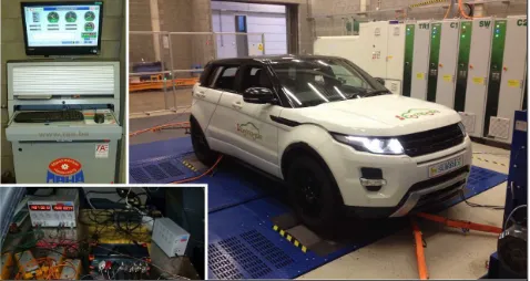
The solution of the wheel torque control allocation problem is based on the experimental data obtained during the characterization of an electric Range Rover Evoque with four identical on-board drivetrains, each of them consisting of a switched reluctance electric motor and a single-speed transmission. Table 1 reports the main vehicle parameters. The experimental tests have been carried out on the MAHA rolling road facility available at Flanders MAKE and at the Lommel proving ground, within the framework of the European project iCOMPOSE [30] (Figure 2).

The experimental power loss characteristics of the left front drivetrain (denoted as drivetrain 1, see Figure 1) in traction conditions are shown in Figure 3 for different vehicle speeds. The power loss, _, , is the difference between the measured electrical input power at the inverter and the mechanical power at the roller of the rolling road. As a consequence, the measured power loss characteristics include the losses in the power electronics (drive), electric motor, mechanical transmission and tire. The tire power losses arise from the rolling resistance (always present) and the longitudinal slip, which varies with the applied torque.

The power loss characteristics are plotted as functions of , i.e., the left front drivetrain output torque. can be expressed as a function of the experimentally measured variables and . is the wheel torque measured at the roller by the rolling road test bench, and is the rolling resistance torque, i.e., the torque that has to be applied by the test bench to keep the wheel in constant velocity conditions on the rolling road when the electric motor torque demand of the drivetrain is zero. includes the effects of tire rolling resistance as well as the drivetrain drag torque occurring in conditions of zero load from the electric motor (for example, the drag torque due to the windage and churning losses within the gearbox). was experimentally measured by applying zero torque demand to the electric motor drive and imposing the desired wheel speed through the test bench. In accordance with the theory [31],

is a function of vehicle speed, . In a first approximation, the quantity / (where is the wheel radius) is the rolling resistance power loss, i.e., the value of _, reported for = 0 in Figure 3. By neglecting the effect of the drivetrain drag torque, it is = + .

4

Figure 2. The vehicle demonstrator set up on the rolling road facility

Figure 3. Experimental power loss characteristics for the left front electric drivetrain for different vehicle speeds

2.2 Effect of the longitudinal and lateral accelerations

Longitudinal and lateral accelerations cause load transfers, which influence the tire rolling resistance and, thus, provoke variations of the power loss characteristics of the drivetrains. Tire slip power losses are neglected here, as their minimization requires advanced and precise state estimators that must be effective also in normal driving conditions, which is not industrially viable at the moment. By using the notations in Figure 4 and disregarding aerodynamic effects, the vertical loads at each wheel are (see Figure 1 for numbering convention):

, = #, −1_{2 ∆} , (− ∆ , ),* (1.a)

,+= #,+−1_{2 ∆} , (+ ∆ , ),* (1.b)

,,= #,,+1_{2 ∆} , (− ∆ , ), (1.c)

0 100 200 300 400 500 600 700 800 900 0

5 10 15 20 25 30 35 40

τ d (Nm)

Plo

ss

,1

(

k

W

)

V (km/h) 20 37.5 75 90 105 120 140

1

Table 1. Vehicle parameters

Symbol Name and unit Value

ℓ Wheelbase (m) 2.665

. Gearbox ratio (-) 10.56

Wheel radius (m) 0.364

/ Half-track (m) 0.808

− No. of motors per axle (-) 2

5

,0= #,0+1_{2 ∆} , (+ ∆ , ), (1.d)

where _#,1 is the static load on the 2-th wheel, ∆ _{, (} is the load transfer caused by the longitudinal acceleration , and ∆ _{, ),*} and

∆ , ), are the load transfers on the front and rear axles, caused by the lateral acceleration 3 in steady-state cornering. In formulas:

∆ , (=

4 5

6 (2.a)

∆ , ),*=

4 3

2/ 7896:,*+;<=;+ ;<= <>?5 − 9 :,: @AB

(2.b)

∆ , ), =

4 3

2/ 7 9 :,

6 +

;<>

;<=+ ;<>?5 − 9 :,: @AB

(2.c)

The notations ;_<= and ;_<> indicate the roll stiffness of the front and rear suspension systems.

Under the hypotheses of this study, the drivetrain power loss characteristics do not include the lateral tire slip power losses. Moreover, the longitudinal slip ratios are considered invariant with respect to the values measured on the rolling road, which means that the longitudinal tire slip power losses do not change from the measured values. As a consequence, the only component of the drivetrain power loss characteristic that changes with the vertical load is the rolling resistance of the tires. Based on [31], the rolling resistance torque is assumed to vary linearly with the vertical load. In addition, the drivetrain drag torque is considered to be negligible compared to the tire rolling resistance, so that:

C ,1D = C #,1D ,1

E,

(3)

where _,1 is defined in Eq. (1). Eq. (3) is obtained from experimental measurements of the actual rolling resistance behavior of tires (see [31]). As a result, the rolling resistance power loss contribution, C _,1D, becomes:

C ,1D = C #,1D ,1

E,

= /1 (4)

C ,1D is the value of ,1 at = 0. Also, as explained in Section 4, C ,1D is the coefficient /1 of the third order

polynomial used for modeling the power loss of the explicit control allocation (E-CA).

As a consequence of Eq. (4), the variation of wheel load induces a variation of rolling resistance, which shifts the power loss characteristics _,1C D vertically. As a result, the power loss characteristics will be different at each vehicle corner. For example, Figure 5 shows the effects of =6 m/s2 and ₃= 2.5 m/s2 on the power loss curves of the four drivetrains of the vehicle demonstrator at V = G0 km/h.

6

Figure 5.Power loss characteristics at each vehicle corner (2 = 1 … 4A at 90 km/h with = 6 m/s2 _and

3= 2.5 m/s2

2.3 Different drivetrains on the front and rear axles

This section discusses the power loss model for the case of front and rear drivetrains with the same speed range but different torque characteristics achieved by scaling. In particular, a constant ratio between the maximum torque values of the front and rear drivetrains is assumed and defined by the scaling factor M > 0. It is also supposed that the power loss characteristics are scaled according to the same parameter M. As a result, the efficiency of the front and rear drivetrains is the same with respect to the normalized torque demand, which is the actual torque divided by the maximum possible value of torque demand for the specific electric drivetrain at a particular speed. This scaling methodology of the efficiency map, already adopted in [32], is not generally applicable, but represents a realistic and instructive assumption for cases where the different drivetrains are based on the same motor technology.

Hence, the power loss characteristic on the left rear drivetrain, which depends on _O, can be expressed as a function of _, ? _O/

MA:

,,C OD = M , P _{M Q + / − / M}O (5)

The term / − / M on the right-hand side of Eq. (5) allows to maintain the same value of rolling resistance power loss on the two drivetrains, as rolling resistance is not affected by M. Figure 6 shows the power loss characteristics of the original and scaled drivetrains with M = 0.5.

Figure 6.Power loss characteristics of the original drivetrains at the front axle (1,2) and the drivetrains scaled with M = 0.5 at the rear axle (3,4) at 90 km/h

3. Problem formulation

3.1 General formulation

The optimal torque distribution among the multiple drivetrains of an electric vehicle can be obtained by solving a multi-parametric nonlinear programming (mp-NLP) problem, which, in general, is formulated as follows [33-34]:

0 100 200 300 400 500 600 700 800 900 0

5 10 15 20 25 30 35 40

τ d (Nm)

Plo

ss

,i

(

k

W

)

1 2 3 4

i

0 100 200 300 400 500 600 700 800 900 0

5 10 15 20 25 30 35 40

τ d (Nm)

Plo

ss

,i

(

k

W

)

1,2 3,4

7

RST∗_{?VA = min}

Z [ ?Z, VA (6.a)

\. ]. ^?Z, VA = 0 (6.b)

9?Z, VA ≤ 0 (6.c)

where [ is the cost function, Z is the vector of optimization variables, V is the vector of parameters, RST∗ is the vector of optimal values, ^ and 9 represent the equality and inequality constraint functions, and the symbol R T∗ indicates the optimality of the solution.

The torque of the 2-th drivetrain is defined as:

= _,`− _,a (7.a)

,` ,a= 0, with 2 = 1,2,3,4 (7.b)

where is the drivetrain output torque, i.e., the torque after the transmission in the case of on-board electric drivetrains. _,`≥ 0 and _,a≥ 0 are the traction and regeneration torques, respectively. Equality (7.b) has to be imposed because each electric drivetrain can only operate in traction or regeneration.

In order to minimize the electric vehicle power losses, the mp-NLP problem in (6) can be re-formulated as:

RdeT∗?VA = arg min_di [ ?de, VA = j 1C , VD 0

1k

(8.a)

\. ]. j =

0

1k

(8.b)

/ C _l− D + / C _m− _OD = _(8.c)

−de,n ,.?VA ≤ de≤ de,n ,o?VA _(8.d)

Vn1p≤ V ≤ Vn _(8.e)

where d_e = q , _l, _O, _mrsis the vector of the drivetrain output torques, ₁ is the electrical power drawn or regenerated by the

2-th drivetrain, and / and / are the front and rear half-tracks. The analysis of ₁C , VD, presented in the next sections, will show that (8) is a non-convex optimization problem.In general, the vector of parameters V can be defined as:

V = q , , 3, t, u, vrs (9)

where t = wx , x₊, x_,, x₀y, u = wz , z₊, z_,, z₀y, and v = w{ , {₊, {_,, {₀y are the vectors of slip angles, slip ratios, and motor temperatures, respectively.

Eqns. (8.b) and (8.c) are the two equality constraints of the mp-NLP problem, i.e., the approximated longitudinal force and yaw moment balance equations of the vehicle for small steering angles. They guarantee that and , the reference longitudinal force and yaw moment from the high-level controller, are actually generated, under the approximation of neglecting the effect of tire rolling resistance on and . The inequality constraints in (8.d) and (8.e) are expressed through the vectors d_{e,n ,o}?VA, −d_{e,n ,.}?VA,

Vn and Vn1p, which represent the maximum and minimum allowed values for de and V. The inequalities are to be interpreted

among the respective elements of the vectors.

3.2 Cost function simplification

8

1= + ,1C , VD (10.a)

,1C , VD = ,1,oC , VD\C D + ,1,.C− , VD\C− D (10.b)

\C D = |1₀ ≥ 0_{< 0} (10.c)

The terms _,1,oC , VD and _,1,.C , VD are the power losses of the 2-th vehicle corner, respectively in traction and regeneration, while \C D is the unit step function. This notation is convenient for describing the power loss characteristics, which may be significantly different in traction and regeneration for the same drivetrain. The energy storage power losses are not considered, as they are increasing functions of the drivetrain input power, and thus irrelevant for wheel torque control allocation. By substituting (10) into the cost function[ ?d_e, VA of (8), it is:

[ ?de, VA = + j ,1C , VD

0

1k

(11)

The term is constant for any d_e; therefore, for the purpose of power loss minimization, the expression of the cost function can be simplified into:

[ ?de, VA = j ,1C , VD

0

1k

(12)

In real-life applications, the individual power loss characteristics of the vehicle corners may be different from each other. For example, as described in Section 2, with four identical electric drivetrains power loss differences can arise due to longitudinal and lateral accelerations. Also, physically different drivetrains on the front and rear axles may yield different power loss characteristics.

3.3 Independence of vehicle sides

As shown in [16] and [28], the mp-NLP problem in (8) can be solved independently for each side of the vehicle. By combining the two expressions in (8.b) and (8.c) and assuming / = / = / , the drivetrain output torques on the left- and right-hand sides of the vehicle, _, and _, , read:

, = + O= 0.5 P − / Q (13.a)

, = l+ m= 0.5 P + / Q (13.b)

Hence, the new cost function [₊Cd_e,~, VD for the left-hand side of the vehicle is defined as:

[+Cde,~, VD = , C , VD+ ,,C O, VD (14)

As a consequence, the optimal torque distribution between the left front and left rear drivetrains is the solution of the following mp-NLP problem:

•de,~€∗?VA = arg min_di,• [+Cde,~, VD (15.a)

\. ]. −de,~,n ,.?VA ≤ de,~≤ de,~,n ,o?VA (15.b)

Vn1p≤ V ≤ Vn (15.c)

where d_e,~= q , _Ors is a vector containing the drivetrain output torques for the left-hand side of the vehicle, and the vectors

de,~,n ,o?VA and −de,~,n ,.?VA represent the maximum and minimum allowed values for de,~. Owing to the independence of the

9

3.4 Optimal traction-regeneration balance on a vehicle side

This section demonstrates that [₊Cd_e,~, VD is minimized if both drivetrains on the same side work either in traction or regeneration, under the hypotheses that _,1,o/.‚ _{,`/a</sub>, Vƒ is positive and strictly monotonically increasing as a function of <sub>,`/a}, i.e.,

,1,o/.‚ ,`/a, Vƒ > 0 and „ ,1,o/.‚ ,`/a, Vƒ /„ ,`/a> 0. These hypotheses were experimentally verified for the vehicle

demonstrator of Figure 2 (see Section 2) and are confirmed by other studies [27]. In terms of torque distribution, four scenarios are possible:

Scenario 1: ≥ 0 …†‡ _O≥ 0 (16.a) Scenario 2: < 0 …†‡ _O< 0 (16.b) Scenario 3: ≥ 0 …†‡ _O< 0 (16.c) Scenario 4: < 0 …†‡ _O≥ 0 (16.d)

Scenarios 1 and 2 represent the pure traction and regeneration cases, while in Scenarios 3 and 4 one drivetrain is in traction and the other one is in regeneration.

Let us suppose that _, ≥ 0 and only one drivetrain is active, for example = _, and _O= 0. By introducing a regenerative torque, ˆ?> 0), at the left rear corner, that drivetrain torque becomes _O,‰Š‹= − ˆ and, thus, _,‰Š‹= _, + ˆ. According to (10), owing to ˆ the additional power drawn by the left front electric drivetrain would be ˆŒ+ ∆ _o? ˆ, VA and, correspondingly, the extra regenerated power by the left rear drivetrain would be ˆŒ− ∆ _.? ˆ, VA. As the difference of the extra front power and rear power is positive, the overall power loss increases. That is, ∆ _o? ˆ, VA = _{, ,o}C _, + ˆ, VD − _{, ,o}C _,, VD > 0 and ∆_.? ˆ, VA =

,,,.? ˆ, VA − ,,,.?0, VA > 0, since ,1,o/. is positive and strictly monotonically increasing as a function of the respective

torque demand.

The same conclusion is valid for _, < 0, i.e., the introduction of traction torque on one of the two left drivetrains would increase the overall power loss on the left-hand side. In conclusion, the drivetrains on the same vehicle side must not work with opposing torques. Note that for this conclusion to be valid, the power loss characteristics are not required to be the same for traction and regeneration.

4. Solution of the control allocation problem

This section discusses the solution of the control allocation problem for electric vehicles with four identical drivetrains without considering the effect of longitudinal and lateral accelerations, which is discussed in Section 5.

4.1 Explicit control allocation (E-CA)

The analytical solutions of the control allocation problem proposed in this study are based on simplifications of the experimental power loss characteristics. In particular, the main hypothesis behind the E-CA is that, for a given V, the power loss characteristic of the 2-th vehicle corner is a cubic polynomial with the generic drivetrain output torque as variable:

,1? , VA = 1?VA ,+ 81?VA ++ •1?VA + /1?VA (17)

By fitting (17) to the curves in Figure 3, it can be observed that ₁, •₁, /₁> 0, 8₁< 0, and 8₁+< 3 ₁•₁ are always true, which means:

• In accordance with the hypothesis in Section 3.4, the characteristics _,1? , VA are strictly monotonically increasing

functions of the drivetrain output torque, . This happens ∀ if •₁> 0, ₁> 0 and 8₁+< 4 ₁•₁.

• The _,1? , VA characteristics have an inflexion point (see their typical shape in Figure 3) for > 0, i.e., they exhibit a

transition between a non-convex shape and a convex shape for > 0. An inflexion point exists for > 0 when

| | | |=

−1. Therefore, as ₁> 0, the coefficient 8₁ must be < 0.

10

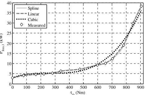
Figure 7. Overlap of the experimentally measured power loss characteristic of the left front drivetrain at 90 km/h and the three investigated fitting functions

In order to find the analytical solution of the control allocation problem (i.e., the E-CA), the output torques at the left front and left rear drivetrains can be expressed as:

= #+ • (18.a)

O= #− • (18.b)

where • is the torque shift with respect to the even distribution, i.e., the case of equally distributed torques between the left front and left rear drivetrains. Hence, _#= _,/2, which is half of the demanded drivetrain output torque for the left side.

By substituting (18) into (15), the control allocation problem can be reformulated as:

R•T∗_{?VA = arg min}

‘ [+?•, #, VA (19.a)

\. ]. − #≤ • ≤ # (19.b)

Vn1p≤ V ≤ Vn (19.c)

Using the cubic polynomial function (17), the expressions of the left front and left rear drivetrain power loss characteristics are substituted into the cost function [₊?•, _#, VA:

[+?•, #, VA = [ˆ?•, #, VA + ? , ? #, VA + ,,? #, VAA = … • + ’•++ “•,+ ? , ? #, VA + ,,? #, VAA (20)

where the constant term _, ? _#, VA + _,,? _#, VA is the power loss associated with the even distribution, and the term

[ˆ?•, #, VA = … • + ’•++ “•, describes the power loss variation induced by the torque shift • with respect to the even torque distribution. The coefficients …, ’ and “ in (20) are given by:

… = 3 #+? − ,A + 2 #?8 − 8,A + • − •, (21.a)

’ = 3 #? + ,A + 8 + 8, (21.b)

“ = − , (21.c)

The minimization of [₊?•, _#, VA can be achieved by minimizing [ˆ?•, _#, VA. By solving ∇_‘[ˆ?•, _#, VA = 0, it is:

•ˆ =−’ + •’_3“+− 3…“ (22)

while the complementary solution –—–˜—l–,™:

,: is discarded as it maximizes [ˆ. If “ = 0, (22) becomes:

•ˆ =–—_+™ if ?“ = 0A AND ?… ≠ 0A (23.a)

•ˆ = 0 if “ = … = 0 (23.b)

0 100 200 300 400 500 600 700 800 900 0

5 10 15 20 25 30 35 40

τ d (Nm)

Plo

ss

,1

(

k

W

)

Spline Linear Cubic Measured

11

The solutions in (22-23) minimize [ˆ only if ’ ≥ 0. The optimal value R•T∗ that minimizes [ˆ has to be sought among •ˆ, •_n1p= − _# and •_n = _#, because •ˆ (if it exists) could be a local minimum or be located outside the domain of •.

If the vehicle has four electric drivetrains with equal power loss characteristics (as the vehicle demonstrator in Figure 2), then

,1? , VA = ? , VA, and thus … = “ = 0 and ’ = 6 _# +28 , according to (21) and the fact that = _,, 8 = 8_,, and

• = •,. In this special case, the optimal solution of (19) for the left-hand side of the vehicle is:

a) R•T∗= − _#› _#, i.e., only one drivetrain should be used for small values of _, (’ < 0 since it is 8 < 0).

b) R•T∗= 0, i.e., even torque distribution between the drivetrains on the same side should be adopted for large values of _, (’ ≥ 0).

c) On a vehicle side the optimal switching torque, _,œ•, between strategies a) and b) is calculated as the solution of ’? _#A = 0:

,œ•= 2 ˆ#= −2?8 + 8_{3? +} ,A ,A = −

28

3 (24)

which is also the solution of the more general expression (from Theorem 1 in [28]):

C ,œ•, VD + ?0, VA = 2 ‚ _{2 , Vƒ},œ• (25)

The same results are valid for the right-hand side of the vehicle as well.

4.2 Implicit control allocation (I-CA)

The implicit control allocation (I-CA) uses an off-line optimization for the solution of problem (15) to generate a map of the energy-efficient torque distribution for each side of the vehicle. The experimental data of the drivetrain power losses are fitted with spline functions (see Figure 7) that reduce fitting errors compared to the third order polynomial of the E-CA. ž =_Ÿ Ÿ_¡Ÿ

O is defined as the

front-to-total drivetrain torque distribution for the left-hand side of the vehicle, i.e., ž = 1 or ž = 0 in the case of single-axle allocation, and ž = 0.5 in the case of even torque distribution. The resulting I-CA map implemented in this study outputs the optimal front-to-total drivetrain torque ratio, RžT∗, as a function of vehicle speed and the demanded drivetrain output torque _, on the specified vehicle side, for example _, = _,. The map of RžT∗ can be computed through different optimization methods, such as Newton-type methods applied to a discretized set of parameters. Figure 8 is the resulting I-CA map for the wheel torque allocation on a vehicle side. Even if the optimal wheel torque distribution according to the I-CA shows more complex behavior than the E-CA, the general trend is towards a single-axle distribution at low torque demands and an even torque distribution at medium-high torque demands.

Figure 8.I-CA: map of RžT∗ as a function of vehicle speed and demanded drivetrain output torque on the vehicle side; the white star represents the point experimentally investigated in steady-state conditions in Section 6

4.3 Hybrid control allocation (H-CA)

The main idea of the hybrid control allocation (H-CA) is to combine the simplicity of the E-CA with the fitting accuracy of the power loss characteristics adopted within the I-CA optimization. Similarly to the E-CA, the H-CA only allows to switch between the single axle and the even distribution at a switching torque which is a function of V. The H-CA calculates the switching torque through Eq. (25). In this study a piecewise linear interpolation of the experimental points in Figure 3 is used for the H-CA switching torque calculation. The piecewise linear interpolation is chosen to show the effect of different levels of approximation of the drivetrain

20 40 60 80 100 120 140

0 100 200 300 400 500 600

V (km/h)

τd,

s

(Nm)

{r}

* (%)

50 55 60 65 70 75 80 85 90 95 100

12

power loss characteristics. The spline approximation of the drivetrain power loss characteristic could be adopted for the H-CA as well.

4.4 Remarks

In the practical implementation of the CA algorithms, the strategies of Sections 4.1-4.3 are overruled in the following cases: i) If wheel torque saturation occurs (e.g., because of the estimated tire-road friction conditions or achievable drivetrain torque), the torque demand beyond the limit is transferred to the other wheel on the same side until saturation is reached as well; ii) For significant decelerations, an electronic braking distribution (EBD) strategy intervenes to maintain the correct relative slip ratio among the tires of the front and rear axles. The details of i) and ii) will be described in future contributions, while this paper is focused on how to reduce drivetrain power losses with simple and computationally efficient CA.

An important note is that the on-line calculations of the E-CA and H-CA are based on a look-up table each for the determination of the switching torque, with vehicle speed as main input (actually there may be other inputs depending on V). The on-line calculations of the I-CA are based on the multi-dimensional look-up table of the optimal front-to-total torque distribution, receiving vehicle speed and drivetrain torque demand on each side as main inputs. All three control allocation methods imply very low on-line computational load, which is a major contribution of this study.

5. E-CA: case studies

The following sections discuss the E-CA solution for the case of the vehicle subject to moderate load transfers in longitudinal and lateral directions, and the case of front and rear drivetrains with the same motor technology but different torque range.

5.1 Effect of the longitudinal and lateral accelerations

Interestingly, in condition of non-zero longitudinal and lateral accelerations the optimal solution of the control allocation problem,

R•T∗_{, using the E-CA is the same as the one derived in Section 4.1, which assumes identical power loss characteristics for the four}

vehicle corners. In fact, according to (4), the variation of vertical load affects only the term /₁ in Eq. (17). As a consequence, there is no change in the term [ˆ of Eq. (20), which does not depend on /₁. Based on this, and ₃ can be removed from V, which becomes

V = in this study.

The invariance of the solution is due to the use of the demanded drivetrain output torque, , as control variable of the optimisation problem. If the optimization problem were defined in terms of = − , after appropriate reformulations of the cost function (see Eqns. (18-19)), it would be:

= ,#+ • (26.a)

O= ,#− • (26.b)

where _,# is half of the desired wheel torque at the side, e.g., for the left side it is _,#= C + _OD/2, while • is the offset from the even wheel torque distribution. By combining = + , Eq. (26) and Eq. (18), • becomes:

• = • + O−

2 (27)

13

Figure 9.E-CA at 90 km/h with = 6 m/s2 _and

3= 2.5 m/s2: (a) optimal front-to-total torque ratio RžT∗; (b) optimal torque shift R•T∗; (c) optimal torque shift R• T∗

5.2 Different drivetrains on the front and rear axles

By using the third order polynomial according to Eq. (17) and under the hypothesis of Eq. (5), the coefficients of _,,? , VA can be related to _, ? , VA:

,=_¢l, 8,=_¢, •,= • , /,= / (28)

After re-arrangements, Eq. (22) becomes:

•ˆ = •ˆ = # –¢_¡¢ if #≥ ‘ (29.a)

•ˆ = •ˆ+= # ¡¢_–¢++_{, –¢}¢ if _#< _‘ (29.b)

where:

‘= −_{6 ?M + 1A}8 (30)

and the front-to-total torque ratios corresponding to (29.a) and (29.b) are respectively:

žˆ = _{1 + M}1 (31.a)

žˆ+= _{1 − M +}1 ₃8 #

M

1 − M (31.b)

As discussed in Section 4.1, the optimal solution R•T∗, which minimizes [ˆ, has to be found among the three values •ˆ, − _# and _#. To do so, the following procedure is employed that starts by considering the condition [ˆ?− _#A < [ˆ? _#A, which is satisfied for:

-100 50 200 350 500 650 800 900 0

25 50 75 100

τ d,s (Nm)

{

r}

* (

%

)

τ d,SW

-1000 50 200 350 500 650 800 900 100

200 300

τ d,s (Nm)

{

ε

}

* (

N

m

)

τ d,SW

-1000 50 200 350 500 650 800 900 100

200 300

τ w,s (Nm)

{

εw

}

* (

N

m

)

τ w,SW

(a)

(b)

14

#≥ £ if M ≥ 1 (32.a)

#< £ if M < 1 (32.b)

where:

£= −₂8 _{M + 1}M (33)

Therefore, the domain of • can be split into two sub-domains. In the first sub-domain, in which [ˆ?− _#A < [ˆ? _#A, the optimal solution is given by:

R•T∗_{= •ˆ if [ˆ?− #A ≥ [ˆ?•ˆA} (34.a)

R•T∗_{= − # if [ˆ?− #A < [ˆ?•ˆA} (34.b)

while in the second sub-domain, in which [ˆ?− _#A ≥ [ˆ? _#A, the optimal solution is:

R•T∗_{= •ˆ if [ˆ? #A ≥ [ˆ?•ˆA} (35.a)

R•T∗_{= # if [ˆ? #A < [ˆ?•ˆA} (35.b)

According to (29), •ˆ is •ˆ or •ˆ₊ depending on the condition _#≷ _‘. Therefore, the conditions in (34) and (35) contain four inequalities, [ˆ?± _#A ≥ [ˆ?•ˆ_/+A. In principle, these inequalities can be expressed in an explicit form, _#≷ ¦₁, where the coefficients ¦₁ are functions of , 8 andM. Specifically, by defining:

¦

™= −₊ ¢¡¢

l

+¢¡ , ¦—= −+ ¢¡

¢¡+, ¦:= −, ¢¡¢l

+?+¢– A, ¦e= −, ¢¡

+?+–¢A (36)

then, for M < 1, the following algorithm (Algorithm 1) provides R•T∗. The four external “if” conditions correspond to the four inequalities [ˆ?± _#A ≥ [ˆ?•ˆ_/+A).

Algorithm 1 – Calculation of R•T∗ for the case of scaled drivetrains among the two axles with M < 1

If _#≥ _‘ AND _#< _£

If _#≥ ¦_™ AND − _#≤ •ˆ ≤ _# Then R•T∗= •ˆ, Else R•T∗= − _# If _#≥ _‘ AND _#≥ _£

If _#≥ ¦_— AND − _#≤ •ˆ ≤ _# Then R•T∗= •ˆ, Else R•T∗= _# If _#< _‘ AND _#< _£

If M < 0.5

If _#< ¦_: AND − _#≤ •ˆ₊≤ _# Then R•T∗= •ˆ₊, Else R•T∗= − _# Elseif M = 0.5

If − _#≤ •ˆ₊≤ _#

Then R•T∗= •ˆ₊, Else R•T∗= − _# Elseif M > 0.5

If _#≥ ¦_: AND − _#≤ •ˆ₊≤ _# Then R•T∗= •ˆ₊, Else R•T∗= − _# If _#< _‘ AND _#≥ _£

If _#< ¦_e AND − _#≤ •ˆ₊≤ _# Then R•T∗= •ˆ₊, Else R•T∗= _#

15

As discussed in Section 2.2, the longitudinal and lateral accelerations affect only /₁ in (17). As a consequence, the optimal solution for non-zero accelerations and scaled drivetrains is identical to the one discussed so far.

Figure 10 shows the optimal front-to-total torque ratio with M = 0.5at 90 km/h.The corresponding values are: _‘= 201 Nm, _£ = 134 Nm, _™¦ = 151 Nm, ¦_—= 241 Nm, and ¦_e= 134 Nm. In this specific case, R•T∗ changes from − _# to _# at _, = 2 ¦_£= 268 Nm, and from _# to •ˆ (žˆ =0.67) at _, = 2 ¦_—= 482 Nm (note that _, = 2 _#).

Figure 10.E-CA: optimal front-to-total torque ratio (in percentage, RžT∗) as a function of the demanded drivetrain output torque on a vehicle side ( _,), at 90 km/h with M = 0.5

6. Results for the case study electric vehicle demonstrator

This section presents a selection of results obtained with the case study Range Rover Evoque with four identical drivetrains, including a critical analysis of the benefits of the three developed CA methods.

6.1 Power loss analysis

Based on the experimentally measured power loss characteristics, Figure 11 compares the power loss on the left-hand vehicle side ( _, = _, + _,,) for the single axle strategy (SA, i.e., traction torque is only provided by the front drivetrain), the even distribution strategy (ED), and the I-CA, at 90 km/h. As expected, for low torque demands the SA strategy is more efficient than the ED, while the opposite is true for medium-high torque demands. The I-CA provides the overall optimal solution that tends to be close to either the SA or ED strategies, whichever provides higher efficiency. This means that the benefit of selecting torque distributions different from single axle or even distribution within a control allocation algorithm is marginal with respect to the simple solutions provided by the E-CA and H-CA. Figure 11 shows that the appropriate selection of the front-to-rear torque distribution consistently provides significant energy savings throughout the full range of torques. For example, at 200 Nm the I-CA coincides with the SA and provides a 10.5% power consumption reduction with respect to the ED, while at 800 Nm the I-CA guarantees 45.8% and 2.4% power consumption reductions compared to the SA and ED, respectively. Figure 12 extends the comparison to the performance of the I-CA, H-CA and E-CA, in decreasing order of energy efficiency, where the differences in terms of power loss among the three control allocations are relatively small and much lower than the differences between the I-CA and the constant distribution strategies in Figure 11. During the study it was verified that this conclusion is valid for any vehicle speed.

0 100 200 300 400 500 600 700 800 900 0

25 50 75 100

τ d,s (Nm)

{

r}

* (

%

)

2 τ

16

Figure 11.Estimated power losses on a vehicle side at 90 km/h for different torque allocation strategies: single axle (SA), even distribution (ED) and I-CA

For completeness, Table 2 compares the switching torque, _,ϥ, calculated for the E-CA and H-CA for the electric Range Rover Evoque demonstrator. The difference in the values is caused by the different fitting functions adopted in the two cases. Although the values in Table 2 for the two strategies are rather different at higher velocities, Figure 12 and the experimental results of Section 6.2 show that this has a negligible effect in most conditions. For example, at 90 km/h the switching torque, _,ϥ, is 536 Nm for the E-CA and 316 Nm for the H-CA, with a marginal effect, visible in Figure 12, in terms of power loss.

Figure 12.Estimated power losses on a vehicle side at 90 km/h for different torque allocation strategies: I-CA, E-CA and H-CA

6.2 Experimental results

This section presents the experimental results obtained with the electric Range Rover Evoque prototype. The controllers described so far were implemented on a dSPACE AutoBox system. For the E-CA and H-CA strategies, the transition between the single axle and even distribution cases was smoothed by means of appropriate sigmoid functions to guard against vehicle drivability issues. For the same reason, hysteresis functions on the switching thresholds from the single axle to the even distribution cases and vice versa were included to prevent frequent torque distribution oscillations for the E-CA and H-CA. Moreover, as specified in Section 4.4, in particular conditions, for example during medium-high braking and when the tire-road friction limits or the drivetrain torque limits

0 100 200 300 400 500 600 700 800 900 5

10 15 20 25 30 35 40 45

τ d,s (Nm)

Plo

ss

,s

(

k

W

)

SA ED I-CA

0 100 200 300 400 500 600 700 800 900 5

7.5 10 12.5 15

τ d,s (Nm)

Plo

ss

,s

(

k

W

)

I-CA E-CA H-CA

Table 2. Switching torque (Nm) at different vehicle speeds: explicit CA (E-CA) and hybrid CA (H-CA)

CA strategy

(km/h)

0 20 37.5 75 90 105 120 140

E-CA 539 539 626 567 536 525 397 0

17

are approached, the control allocation strategies can be overruled by the electronic brake distribution algorithm, the individual wheel slip controllers or other safety-critical algorithms.

As a first study, the effectiveness of the I-CA was verified through steady-state rolling road tests at different front-to-total torque ratios, yet unchanged overall output torque and speed. For example, for the operating point corresponding to the white marker in Figure 8, at _, = 520 Nm and = 105 km/h, according to the I-CA it is RžT∗= 0.67. The measured electric motor power inputs with SA, ED and I-CA are 104.82 kW, 102.60 kW and 102.37 kW, where the respective values of the efficiency are 0.7553, 0.7678 and 0.7681. This confirms the correct tuning of the I-CA for steady-state conditions.

Figure 13.Speed profile of the SDDC

To evaluate the CA strategies, the vehicle prototype was tested along four driving cycles: i) the New European Driving Cycle (NEDC); ii) the Artemis Road driving cycle; iii) the Extra Urban Driving Cycle (EUDC, this cycle was run with an emulated uphill constant road slope of 8%); and iv) a newly introduced driving cycle, namely the Surrey Designed Driving Cycle (SDDC), see Figure 13. The SDDC was conceived to emphasize the effect of the control allocation on the energy consumption, and to assess the difference between E-CA, I-CA and H-CA. In fact, for the conventional driving cycles assuming a horizontal road, the torque distributions chosen by the presented control allocation algorithms tend to be close to the single-axle distribution. This behavior is due to rather low torque demand and the very high power rating of the electric motors installed on the vehicle demonstrator. In other words, an electric vehicle with less powerful drivetrains would not show this phenomenon. In order to achieve consistency in the results, a driver model, based on the combination of feedforward and feedback control of vehicle speed, was implemented onto the dSPACE system to accurately follow the speed profile of the driving cycles, by varying the torque demand (including braking). Figure 14 reports the switching thresholds for the E-CA and the H-CA (shown in Table 2) as functions of vehicle speed, and the operating point distribution in terms of drivetrain torque demand for each vehicle side during the SDDC.

Figure 14.Experimental points of the SDDC and switching torques for E-CA and H-CA

The numerical results of the experiments are reported in Table 3. The main observations are:

• For all driving cycles, the CA strategies lead to reduced energy consumption with respect to the SA and ED strategies.

0 50 100 150 200

0 20 40 60 80 100 120 140

Time (s)

V

(

k

m

/h

)

0 20 40 60 80 100 120 140

0 150 300 450 600 750

V (km/h)

τd

,s

(

N

m

)

E-CA: τ d,SW

H-CA: τ d,SW

18

• For the NEDC and Artemis Road driving cycle the average torque demand level is moderate, and the optimal solution is

very close to the SA strategy. Therefore, the CA strategies provide a small improvement with respect to the SA strategy, and greater improvement with respect to the ED.

• For the EUDC with the emulated uphill slope the average torque demand level is relatively high and the optimal solution is

very close to the ED. Therefore, the CA strategies provide a small improvement with respect to the ED, and greater improvement with respect to the SA strategy.

• For the SDDC all control allocation strategies provide a significant improvement (> 2%) compared with the SA and ED

cases.

• Differently from the steady-state experimental analysis, the I-CA is not the best strategy in actual operating conditions,

because it requires continuous changes to the front-to-rear torque distribution, yielding drivetrain oscillations that compromise vehicle drivability and also (marginally) energy efficiency.

• Despite the significant difference between E-CA and H-CA in terms of the switching thresholds for the transition from the

single axle operation to the even distribution operation (see Figure 14 and Table 2), the actual difference in the energy consumption results is negligible, with an overall marginal benefit for the H-CA.

• In the authors’ opinion, the conclusion of the driving cycle analysis is that the H-CA represents the best compromise

between off-line computational simplicity and accuracy, ease of vehicle implementation, and energy efficiency, and is actually recommended among the different CA solutions proposed in this paper for electric vehicles with identical drivetrains.

19

Table 4. Energy consumption during steady-state cornering tests at 39 km/h and 79 km/h (60 m radius) with different torque allocation strategies: single axle (SA), even distribution (ED), hybrid CA (H-CA)

Vehicle speed

Reference yaw moment

Control allocation

strategy

Power input

Power input difference with

respect to SA

Wheel torque demand

Front-to-total torque distribution

Left Right Left Right

39 km/h 300 Nm

SA 7.35 kW NA

56 Nm 193 Nm

SA SA

ED 7.72 kW 5.03% ED ED

H-CA 7.35 kW NA SA SA

79 km/h 825 Nm

SA 54.46 kW NA

171 Nm 542 Nm

SA SA

ED 54.22 kW -0.44% ED ED

H-CA 53.15 kW -2.40% SA ED

7. Conclusion

The theoretical and experimental analysis of this paper allows the following conclusions:

• For the case study electric vehicle, a fitting model based on a cubic polynomial is a good approximation of the drivetrain

power loss characteristic as a function of the drivetrain torque demand. Based on published studies, this fitting method of the power loss curves is applicable to a wide range of electric drivetrains.

• The analytical solution of the control allocation problem can be explicitly achieved from the coefficients of the proposed

third order fitting model, including consideration of load transfers and different drivetrains on the front and rear axles.

• In a first approximation, the load transfer caused by the longitudinal and lateral accelerations provokes a linear variation of

the rolling resistance power loss, but it does not change the optimal front-to-total drivetrain torque distribution.

• Experimental tests with different driving cycles demonstrate the effectiveness of the explicit control allocation strategy,

providing results very close to those of more sophisticated control allocation strategies, the so-called implicit control allocation and hybrid control allocation, requiring off-line numerical optimizations.

• The implicit control allocation strategy computes more efficient torque distribution between the front and rear axles in

steady-state conditions, as confirmed by the experiments. However, the continuous variation of the torque distribution observed during the driving cycles introduces drivability issues and a marginal increase of the energy consumption.

• Despite not being explicitly designed for cornering conditions, for lateral accelerations between 2 m/s2 and 8 m/s2 the hybrid

control allocation algorithm brings experimentally measured energy savings of up to 5%, with respect to the single axle and/or even distribution cases.

• The hybrid and explicit control allocation strategies provide a good balance between low on-line computational burden,

Table 3. Energy consumption along driving cycles with different torque allocation strategies: single axle (SA), even distribution (ED), implicit CA (I-CA), explicit CA (E-CA), hybrid CA (H-CA)

Driving cycle

Energy consumptions

Improvement by

I-CA with respect to

E-CA with respect to

H-CA with respect to

SA ED I-CA E-CA H-CA SA ED SA ED SA ED

NEDC 2.932 kWh 3.031 kWh 2.921 kWh 2.920 kWh 2.923 kWh 0.38% 3.63% 0.41% 3.66% 0.31% 3.56%

Artemis Road 4.577 kWh 4.669 kWh 4.549 kWh 4.527 kWh 4.532 kWh 0.61% 2.57% 1.09% 3.04% 0.98% 2.93%

EUDC

8% slope 5.838 kWh 5.739 kWh 5.730 kWh 5.716 kWh 5.716 kWh 1.85% 0.16% 2.09% 0.40% 2.09% 0.40%

20

simple off-line calculations, high energy efficiency during real vehicle operation, and predictable torque distributions. In particular, given its accuracy in the off-line interpolation of the drivetrain power loss characteristics, the hybrid control allocation is recommended by the authors for further industrial implementation in case of electric vehicles with identical drivetrains.

Acknowledgements

The research leading to these results has received funding from the European Union Seventh Framework Programme FP7/2007-2013 under Grant Agreement No. 608897 (iCOMPOSE project).

References

1. L. De Novellis, A. Sorniotti, P. Gruber, J. Orus, J.M. Rodriguez Fortun, J. Theunissen and J. De Smet, "Direct yaw moment control actuated through electric drivetrains and friction brakes: Theoretical design and experimental assessment,"

Mechatronics, vol. 26, pp. 1-15, 2015.

2. L. De Novellis, A. Sorniotti and P. Gruber, "Wheel Torque Distribution Criteria for Electric Vehicles With Torque-Vectoring Differentials," IEEE Transactions on Vehicular Technology, vol. 63, no. 4, pp. 1593-1602, 2014.

3. Q. Lu, P. Gentile, A. Tota, A. Sorniotti et al., "Enhancing vehicle cornering limit through sideslip and yaw rate control,"

Mechanical Systems and Signal Processing, vol. 75, pp. 455-472, 2016.

4. T. Goggia, A. Sorniotti, L. De Novellis, A. Ferrara et al., "Integral sliding mode for the torque-vectoring control of fully electric vehicles: theoretical design and experimental assessment," IEEE Transactions on Vehicular Technology, vol. 64, no. 5, pp. 1593-1602, 2015.

5. L. De Novellis, A. Sorniotti and P. Gruber, "Optimal wheel torque distribution for a four-wheel-drive fully electric vehicle,"

SAE International Journal of Passenger Cars-Mechanical Systems, vol. 6, no. 1, 2013-01-0673, pp. 128-136, 2013.

6. Y. Chen and J. Wang, "Adaptive Energy-Efficient Control Allocation for Planar Motion Control of Over-Actuated Electric Ground Vehicles," IEEE Transactions on Control Systems Technology, vol. 22, no. 4, pp. 1362-1373, 2014.

7. Y. Suzuki, Y. Kano and M. Abe, "A study on tyre force distribution controls for full drive-by-wire electric vehicle," Vehicle System Dynamics, vol. 52, supp. 1, pp. 235-250, 2014.

8. B. Li, A. Goodarzi, A. Khajepour, S.K. Chen and B. Litkouhi, "An optimal torque distribution control strategy for four-independent wheel drive electric vehicles," Vehicle System Dynamics, vol. 53, no. 8, pp. 1172-1189, 2015.

9. R. de Castro, M. Tanelli, R. Esteves Araújo and S.M. Savaresi, "Design of safety-oriented control allocation strategies for overactuated electric vehicles," Vehicle System Dynamics, vol. 52, no. 8, pp. 1017-1046, 2014.

10. A. Wong, D. Kasinathan, A. Khajepour, S.K. Chen and B. Litkouhi, "Integrated torque vectoring and power management framework for electric vehicles," Control Engineering Practice, vol. 48, pp. 22-36, 2016.

11. T.A. Johansen and T.I. Fossen, "Control allocation - A survey," Automatica, vol. 49, pp. 1087-1103, 2013.

12. O. Härkegård and S. T. Glad, "Resolving actuator redundancy - optimal control vs. control allocation," Automatica, vol. 41, pp. 137-144, 2005.

13. M. Bodson, "Evaluation of optimization methods for control allocation," Journal of Guidance, Control, and Dynamics, vol. 25, no. 4, pp. 703-711, 2002.

14. J. Kang, and H. Heo, "Control allocation based optimal torque vectoring for 4WD electric vehicle," SAE Technical Paper 2012-01-0246, 2012.

15. L. Xiong and Z. Yu, "Control allocation of vehicle dynamics control for a 4 in-wheel-motored EV," IEEE Power Electronics and Intelligent Transportation System Conference (PEITS), Vol. 2, pp. 307-311. IEEE, 2009.

16. A. Pennycott, L. De Novellis, A. Sabbatini, P. Gruber and A. Sorniotti, "Reducing the motor power losses of a four-wheel drive, fully electric vehicle via wheel torque allocation," Proceedings of the Institution of Mechanical Engineers, Part D: Journal of Automobile Engineering, vol. 228, no. 7, pp. 830-839, 2014.

17. X. Yuan and J. Wang, "Torque Distribution Strategy for a Front- and Rear-Wheel-Driven Electric Vehicle," IEEE Transactions on Vehicular Technology, vol. 61, no. 8, pp. 3365-3374, 2012.

18. Y. Chen and J. Wang, "Fast and Global Optimal Energy-Efficient Control Allocation With Applications to Over-Actuated Electric Ground Vehicles," Control Systems Technology, IEEE Transactions on Control Systems Technology, vol. 20, no. 5, pp. 1202-1211, 2012.

19. Y. Chen and J. Wang, "Design and Experimental Evaluations on Energy Efficient Control Allocation Methods for Overactuated Electric Vehicles: Longitudinal Motion Case," IEEE/ASME Transactions on Mechatronics, vol. 19, no. 2, pp. 538-548, 2014. 20. P. Tøndel and T.A. Johansen, "Control allocation for yaw stabilization in automotive vehicles using multiparametric nonlinear

programming," American Control Conference, 2005.

21

22. Z. Dimitrova and F. Maréchal, "Techno–economic design of hybrid electric vehicles and possibilities of the multi-objective optimization structure," Applied Energy, vol. 161, pp. 746-759, 2016.

23. W. Shabbir and S.A. Evangelou, "Real-time control strategy to maximize hybrid electric vehicle powertrain efficiency," Applied Energy, vol. 135, pp. 512-522, 2014.

24. C. Hou, M. Ouyang, L. Xu and H. Wang, "Approximate Pontryagin’s minimum principle applied to the energy management of plug-in hybrid electric vehicles," Applied Energy, vol. 115, pp. 174-189, 2014.

25. J.L. Torres, R. Gonzalez, A. Gimenez, and J. Lopez, "Energy management strategy for plug-in hybrid electric vehicles. A comparative study," Applied Energy, vol. 113, pp. 816-824, 2014.

26. R. Wang, Y. Chen, D. Feng, X. Huang and J. Wang, "Development and performance characterization of an electric ground vehicle with independently actuated in-wheel motors," Journal of Power Sources, vol. 196, no. 8, pp. 3962-3971, 2011.

27. S. Kohler, A. Viehl, O. Bringmann and W. Rosenstiel, "Energy-efficient torque distribution for axle-individually propelled electric vehicles," IEEE Intelligent Vehicles Symposium, 2014.

28. A.M. Dizqah, B. Lenzo, A. Sorniotti, P. Gruber et al., "A Fast and Parametric Torque Distribution Strategy for Four-Wheel-Drive Energy-Efficient Electric Vehicles," IEEE Transactions on Industrial Electronics, vol. 63, no. 7, pp. 4367-4376, 2016. 29. Y. Tang, "Method of operating a dual motor drive and control system for an electric vehicle," US Patent 2013/0241445 A1,

2013.

30. http://www.i-compose.eu/iCompose/, last accessed on 7th July 2016.

31. G. Genta, Motor vehicle dynamics: modeling and simulation, World Scientific, 1997.

32. F. Di Nicola, A. Sorniotti, T. Holdstock, F. Viotto et al., "Optimization of a Multiple-Speed Transmission for Downsizing the Motor of a Fully Electric Vehicle," SAE International Journal of Alternative Powertrains, vol. 1, no. 1, pp. 134-143, 2012. 33. L.F. Domínguez, D.A. Narciso and E.N. Pistikopoulos, "Recent advances in multiparametric nonlinear programming,"

Computers & Chemical Engineering, vol. 34, no. 5, pp. 707-716, 2010.

34. A. Grancharova and T.A. Johansen, "Multi-parametric Programming, in Explicit Nonlinear Model Predictive Control - Theory and Applications," Springer: Berlin Heidelberg, pp. 1-37, 2012.

35. C. de Boor, A Practical Guide to Splines, Springer-Verlag, 1978.

Appendix

Algorithm 1b – Calculation of R•T∗ for the case of scaled drivetrains among the two axles with M > 1

If _#≥ _‘ AND _#< _£

If _#≥ ¦_— AND − _#≤ •ˆ ≤ _# Then R•T∗= •ˆ, Else R•T∗= _# If _#≥ _‘ AND _#≥ _£

If _#≥ ¦_™ AND − _#≤ •ˆ ≤ _# Then R•T∗= •ˆ, Else R•T∗= − _# If _#< _‘ AND _#< _£

If M < 2

If _#< ¦_e AND − _#≤ •ˆ₊≤ _# Then R•T∗= •ˆ₊, Else R•T∗= _#

Elseif M = 2 If − _#≤ •ˆ₊≤ _#

Then R•T∗= •ˆ₊, Else R•T∗= _# Elseif M > 2

If _#≥ ¦_e AND − _#≤ •ˆ₊≤ _# Then R•T∗= •ˆ₊, Else R•T∗= _# If _#< _‘ AND _#≥ _£