Mathematical model for optimising the performance of a ground source heat pump

Mathematical model for optimising the performance of a

ground source heat pump.

PALLEDA, Siva Prakash.

Available from Sheffield Hallam University Research Archive (SHURA) at:

http://shura.shu.ac.uk/20159/

This document is the author deposited version. You are advised to consult the publisher's version if you wish to cite from it.

Published version

PALLEDA, Siva Prakash. (2009). Mathematical model for optimising the

performance of a ground source heat pump. Masters, Sheffield Hallam University (United Kingdom)..

Copyright and re-use policy

jj Sheffield S1 1WD [

1 0 1 9 6 3 6 6 7 X

ProQuest Number: 10697466

All rights reserved

INFORMATION TO ALL USERS

The quality of this reproduction is dependent upon the quality of the copy submitted.

In the unlikely event that the author did not send a com plete manuscript and there are missing pages, these will be noted. Also, if material had to be removed,

a note will indicate the deletion.

uest

ProQuest 10697466

Published by ProQuest LLC(2017). Copyright of the Dissertation is held by the Author.

All rights reserved.

This work is protected against unauthorized copying under Title 17, United States C ode Microform Edition © ProQuest LLC.

ProQuest LLC.

789 East Eisenhower Parkway P.O. Box 1346

MATHEMATICAL MODEL FOR OPTIMISING THE PERFORMANCE OF A GROUND SOURCE HEAT PUMP

E3y

Siva Prakash Palleda

The thesis is submitted in partial fulfilment of the requirement of Sheffield Hallam University for the degree of Master of Philosophy

Abstract

Energy demand for the twenty first century is expected to increase many fold along with corresponding diversification of energy sources and generation methods. Of the many energy sources available, use of Ground Source Heat Pump (GSHP) system is the focus of the analysis in this research.

This work is carried out to identify the key parameters which affect the performance of the GSHP system. A mathematical model has been developed to understand the complex operation of the heat pump under typical working conditions. Individual sub-systems, such as Ground Heat Exchanger (GHE), evaporator, condenser, compressor and radiator are modelled in MathCAD and coupled together and solved simultaneously. The performance of the system is predicted while varying air temperature, power input to the compressor and the ground temperature beneath the earth's surface. In addition a special sub-model was developed for the single vertical U-tube GHE in FLUENT, a Computational Fluid Dynamics (CFD) software, to calculate the overall heat transfer coefficient for varying outer surface temperature of the borehole.

The overall system results are validated against the published results with the system operating range of 18°C to 33°C with around 10 percent deviations.

It is determined that the COP of the system increases with surface area and overall heat transfer coefficient (OHTC) of the heat exchanger. An increase in up to 500 m2 surface area, steep raise of COP from 10.05 to 10.3 is observed. Similarly increase of 10 W/m2K of OHTC has steep COP rise from 10.05 to 10.28. The temperature gradient across the system also has influence on its operating performance, where a 15°C increase in the ground temperature for cooling mode reduces the COP by around 5%. Finally the degree of refrigerant sub-cooling has a positive effect, for every 5°C temperature drop the COP improves by 0.5 similarly for degree of super-heating, COP improves by 0.25.

Contents

Structure of the Thesis... 1

Chapter 1

1.1 Ground temperature variations...6

1.2 Types of GSHP configurations...9

1.3 Cost comparison... 11

1.4 Typical Heat pump cycle operation...13

1.5 Role of GSHP in reducing C02 emissions...14

1.6 Methodology... 17

1.7 Research objectives...21

1.8 Block diagram of the project...23

Conclusion... 24

Chapter 2

2.1 Literature Review...25

2.1.1 Coefficient of Performance (COP)...28

2.1.2 Ground Heat Exchanger (U tubes)... 30

2.1.3 Condenser and evaporator...34

2.1.4 Methodologies used to model the Heat Pump System...36

2.1.4.1 Ground temperature variation modelling... 38

2.1.4.2 Thermal loading on the borehole...41

2.1.4.3 Heat transfer modelling of GHE...44

2.1.5 Development of GSHP...51

2.1.6 Refrigerant... 53

2.1.7 Scope and limitations...59

2.1.8 Computational Fluid Dynamics (CFD)...60

2.1.9 MathCAD... 65

Conclusion... 66

Chapter 3

3.1 Steady state of analytical model...67

3.1.1 GSHP system... 68

3.1.1.2 Heat Pump system...72

3.1.1.3 Compressor...72

3.1.1.4 Evaporator...73

3.1.1.5 Throttle valve...74

3.1.1.6 Radiators...76

3.1.1.7 Room wall...77

3.1.2 Calculation of Thermal resistance... 79

3.1.3 Solving procedure... 83

Conclusion... 85

Chapter 4

4.1 CFD modelling in FLUENT...86

4.1.1 Modelling the U-tube...86

4.1.1.2 Meshing...90

4.1.1.3 Boundary condition and Solving... 91

Conclusion... 92

Chapter 5

5.1 Results and discussions...93

5.1.1 Results from the analytical model...94

5.1.2 Validation with experimental model (Bench mark model)...96

5.1.3 Comparison with Ideal Carnot COP...99

5.1.4 Parametric study...100

5.1.5 CFD model... 106

Conclusion... 109

Chapter 6

6.1 Conclusion and future scope of work...110

6.2 Future scope of work... 113

Conclusion... 114

References... 115

Appendix A - Numerical values for the variables...122

Appendix B: Calculation of Overall Heat transfer Coefficient for heat exchangers ...124

List of Figures

Figure 1 Renewable energy delivered by a heat pump system with COP of 4 ...5

Figure 2 Monthly variation of outdoor air temperature Erzurm, Turkey...7

Figure 3 Monthly variation of mean ground temperatures at several depths Erzurum, Turkey...7

Figure 4 Temperature variations with depth of ground... 8

Figure 5 Horizontal closed loop heat pump system... 10

Figure 6 Horizontal closed loop slinky coil system... 10

Figure 7 Vertical U tube closed loop heat pump system... 11

Figure 8 Capital costs for different configurations... 12

Figure 9 Typical Heat Pump Unit...13

Figure 10 Comparison of several renewable energy techniques... 15

Figure 11 Comparison of fuel costs and C02 emissions for GSHPs and fossil fuel Boilers... 16

Figure 12 Comparison of carbon dioxides emissions from GSHPs and other forms of heating... 17

Figure 13 Flow chart for the project...23

Figure 14 Vertical U-tube in symmetry plane... 30

Figure 15 Basic configurations of Vertical U tubes... 31

Figure 16 Basic configurations of vertical U tubes... 31

Figure 17 Evolution of daily average subterranean temperature and outdoor air temperature...33

Figure 18 Evolution of daily average temperatures of outdoor air, circulating water, surface of ground heat exchanger...34

Figure 19 Typical Plate Heat Exchanger...36

Figure 20 SGSHP System pumping efficiently required pumping water to cooling capacity... 38

Figure 21 Earth temperature distribution surrounding buried coil at different depth after 4 hour operation of GSHP...39

Figure 22 Earth temperature variation with the operation time of GSHP at a depth of 5 m for different radius...40

Figure 24 Borehole loading profile against a dimensionless parameter (z-d/H) (with

value one at bottom and zero at borehole top)... 42

Figure 25 GHE thermal load as a function of the load duration with the inlet and out let temperatures of water at 10°C initial ground temperature...43

Figure 26 The GHE thermal load as a function of the load duration with the inlet and outlet temperatures of water as parameter 15°C intial ground temperature ... 44

Figure 27 Shape factors for three different positions... 47

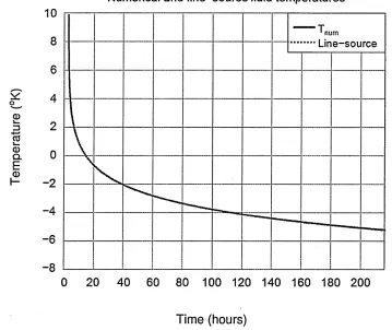
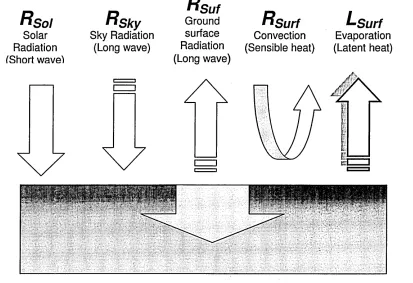
Figure 28 Mean fluid temperature: numerical and theoretical line-source solution48 Figure 29 Thermal balance on ground surface... 50

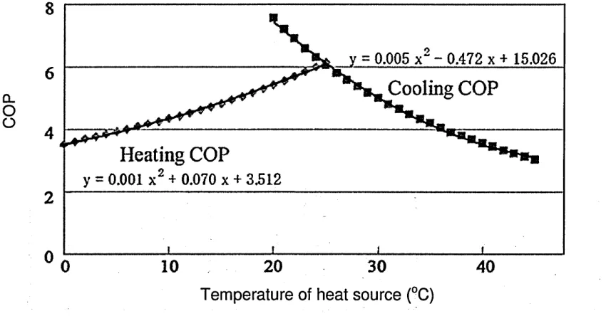
Figure 30 Variation of COP with increase in the temperature of heat source... 51

Figure 31 Refrigerants with ODP and GWP values ...54

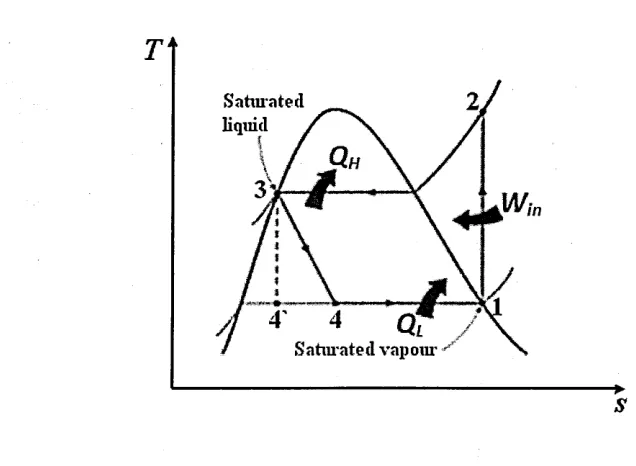
Figure 32 Temperature entropy diagram for refrigerant cycle...55

Figure 33 Pressure enthalpy diagram for refrigerant cycle...56

Figure 34 The three dimensions of computational fluid dynamics...60

Figure 35 Basic structure of the CFD modelling tree.. ... 62

Figure 36 Line diagram of GSHP system... 69

Figure 37 Line diagram of GHE...71

Figure 38 Line diagram of condenser... 72

Figure 39 Line diagram of heat pump system... 73

Figure 40 Line diagram of evaporator... 74

Figure 41 Line diagram of Throttle value... 75

Figure 42 Line diagram of Radiator...76

Figure 43 Line diagram of heat transfer through wall... 79

Figure 44 Various components within the system with their UA values...82

Figure 45 Pipe and water geometry in GAMBIT... 88

Figure 46 Pipe geometry with grout in GAMBIT... 89

Figure 47 Meshed geometry water in the pipe... 91

Figure 48 COP varying with temperature gradient with Tg at 18°C...94

Figure 49 COP varying with temperature gradient with Tair at 33°C...95

Figure 50 Experimental and actual COP for varying compressor power...96

Figure 53 Variation of COP with area of grout... 100

Figure 54 Varying outlet temperature of water from the GHE with area of grout 101 Figure 55 Effect of degree of super heat on COP... 102

Figure 56 Effect of degree of sub cooling on COP... 103

Figure 57 P-h diagram with sub cooling and super heating for a typical cycle... 104

Figure 58 Variation of COP with U value of grout... 105

Figure 59 Contours of temperature distribution in the pipe... 106

Figure 60 Contours of velocity profile in the pipe... 107

Figure 61 Contours of velocity in U tube... 108

Nomenclature

A = Surface area of heat transfer (m2)

Cp = Specific heat ( J/kg K)

d = Diameter of pipe(m)

h = Enthalpy ( J/Kg K)

hf = Convective heat transfer coefficient (W/m2K)

k = Thermal conductivity(W/m K)

KpjPe=Thermal conductivity of pipe (W/m K)

Kgrout=Thermal conductivity of grout (W/m K)

Kground=Thermal conductivity of ground (W/m K)

I = length of pipe (m)

M = Mass flow rate (Kg/s)

mi = Mass flow rate of radiator water (Kg/s)

n = Number of bore holes

Qsr = Cooling load (Watts)

Qs = Condenser load (Watts)

Re = Reynolds number

ri=lnternal radius of pipe(m)

r2=External radius of pipe(m)

r3=External radius of grout(m)

r4=External radius of ground (m)

Tgir = Outside air temperature (°C)

T = Temperature (°C)

v = Velocity of water (m/s)

Win = Power input (Watts)

W1 = Radiator loop circulating water (Kg/s)

List of symbols

ATLm = Log Mean Temperature Difference (°K)

p = Density of water (Kg/m3)

p = Dymanic viscosity (Kg/m s)

Subscripts

ai = Air inside

ao = Air outside

fi = Water inlet to heat pump (°C)

fo = Water outlet from heat pump(°C)

g = Grout

in = Water inlet temperature to the radiator(°C)

out = Water exit temperature from the radiator(°C)

r - Room

ref = Refrigerant

w = Wall

W = Water

1 = Condenser side

2 = Evaporator side

DECLARATION

This thesis is submitted in partial fulfilment of the requirements of Sheffield Hallam

University for the degree of Master of Philosophy. It contains an account of

research carried out between October 2007 to October 2009 in Materials

Engineering and Research Institute, Sheffield Hallam University under the

supervision of Dr Andy Young and Dr Saud Ghani. Except where

acknowledgement and reference is appropriately made, this work is, to the best of

my knowledge, original and has been carried out independently. No part of this

thesis has been, or is currently being submitted for any degree or diploma at this

ACKNOWLEDGMENTS

I would like to acknowledge the support and encouragement of my director of

studies Dr Andy Young and Dr Saud Ghani during the course of this research

project. I also acknowledge the Materials Engineering and Research Institute and

the Faculty of Arts Computing Engineering and Sciences at Sheffield Hallam

University for the provision of computing facilities.

My special thanks extend to Kasara farahani for his unfailing help in using

MathCAD and I would like to thank Dr. Osman Baig and Dr. Ben Hughes for their

constructive ideas and discussions.

I thank all the technical staff in the Materials Engineering and Research Institute

for their help and assistance during the course of research work. Special thanks

are extended to Professor Doug Cleaver and Mrs. Rachael Ogden.

Thanks are also extended to my family and my dear friends Shivaraj Alavandimath

and Narasimha Raju for their unfailing support and encouragement. I also want to

Dedicated to

My beloved Parents

Palleda Thipperudra Swamy

Structure of the Thesis

Chapter

This chapter gives the initiation of the project, answering why this topic has been

chosen and sufficient information about the scope and the developments in the

recent past. It is also introduces to the availability of the non-conventional energy

resources and its applications and research objectives. The block diagram of the

research carried out has been explained.

Chapter

In this chapter the detailed work undertaken by many authors and the

methodologies used to represent the system is discussed in detail. The progress

in the area of GSHP has been highlighted at appropriate instances. There have

been many attempts to develop analytical model of the system and the true

representation of the model in the numerical form as well. Numerous numerical

procedures available to solve the system especially the ground surrounding the

vertical U tube heat exchangers have been discussed. Calculation methods of the

thermodynamic properties of the refrigerant adopted by different authors have

been discussed.

Chapter 3

Each sub system of the GSHP is modelled representing heat balance and heat

transfer equations. Overall there are five heat exchangers in the complete system.

is modelled in Log Mean Temperature Difference (LMTD) method, they are

nonlinear in nature. Theses equations are solved simultaneously with some good

initial guess work. Once the model is established, the variables are fine tuned to

match with the published data. The validated model is used to calculate the new

values of COP. With increase in the surface area of ground heat exchanger and

better thermal properties for the pipe and grout material, the expected COP is

much improved.

Chapter 4

FLUENT is versatile CFD software, used to model and analyse the complex

physical problems. Methodology is developed to model, analyse the GHX and use

results from Chapter 3, and the boundary conditions were used from the published

data for the analysis. The value of the thermal resistance of the grout and pipe

material is used in the analytical model to verify the results. This chapter explains

conditions used to model the system, mesh quality and solution techniques.

Different configurations are modelled to increase the surface area of heat transfer

to observe the effect on COP of the system. Thermal properties of the grout and

pipe material are improved to observe the improvement in the COP of the overall

system.

Chapter

Results from the analysis are discussed and the comparison is made with the

published data to represent the reference model. Normal operating parameters are

Chapter

Conclusions are made with reference to the influence of operating parameters and

the assumptions made. Power input to the compressor, Air temperature and

Ground temperature are the three main variables which drives the system. Water

inlet temperature, degree of superheating and sub cooling effect is also

considered as variables and appropriate conclusions were made for the hybrid

model

Chapter 7

It is out of the scope of the work to implement all the practical operating and time

varying parameters in the current study. Ground modelling for the grout and time

variations might be a good approach for better understanding of the system.

Different configuration of the ground pipe is worth the try. Future suggestions are

Chapter 1

Introduction

Generating power to meet the growing demand of the developing world with

limited resources calls for more efficient, safe, economical and environmental

friendly means and has been a growing challenge for many years. Various non-

conventional methods to generate power and heat from natural resources have

been developed. They are wide spread from wind turbines, solar energy systems

to tidal power systems. Air Source Heat Pumps (ASHP) and geothermal heat

pump systems are environment friendly and greener energy systems. Generally

the geothermal heat pumps are also called as geo-exchange systems. Ground-

Source Heat Pump (GSHP) system uses ground as source or sink and this very

basic energy exchange distinguishes the technology from air-source heat pumps.

Since ASHP uses air as source or sink for the thermal energy exchange for

heating or cooling, auxiliary heating sources are used as its efficiency and capacity

decrease with outside air temperature [1].

GSHP can be used in almost any region, irrespective of any weather conditions.

GSHP uses energy well below the earth surface, which is unaffected by the

outside air temperature, hence it is more reliable technology compared to ASHP.

Mechanical pumps were used directly to circulate the high underground

temperatures water available like hot springs and steam vents for heating indoor

spaces without the use of a heat pump system. Systems such as mechanical

ventilation heat recovery system MVHR show the scope available to develop

In developed countries, approximately 40% of the total energy consumed is

account for space heating and cooling [3]. With the increasing demand for the

power, use of fossil fuel has a greater concern over global warming due to harmful

emissions. Every effort is being made to develop and use energy efficient,

environmentally friendly and less maintenance systems. This need gives rise to

the development of the GSHP system for its less maintenance costs compared to

the conventional alternatives available.

Today GSHP systems are considered to be one of the widely accepted systems in

the renewable energy sector. Around one million GSHP system units have been

installed worldwide in about 30 countries with annual increases of 10% over the

period of last 10 years [4]. Energy consumption is reduced up to 50% in cooling to

70% in heating mode can be observed [5]. This potential for significant energy

savings has led to the use of GSHPs in a variety of applications.

25% Electricity Heat

Pump

100% Delivered Heat

75% Renewable Geothermal Energy

Figure 1 Renewable energy delivered by a heat pump system with COP of 4

The performance of the heat pump system is measured in Coefficient Of

Performance (COP) as that is the ratio of work done to the energy supplied. In

than one, but ASHP with defrost cycle COP can be less than one. The drop in

performance can be accounted for the energy consumed to defrost the heat

exchanger exposed to the outside air. The ranges of COP for practical application

are around 3 to 5; the output is 3 to 5 times the power input to the compressor [6].

As shown in Figurel, these heat pumps with external energy input, cause the heat

to flow from a lower temperature region to higher temperature region, which is the

refrigeration unit that is being used other way round as heat pump system. The

use of heat pump technology is not new, in 1852 Lord Kelvin developed the

concept and Robert Webber was then modified as a GSHP in the 1940s. Duing

1960s and 1970s these heat pumps gained commercial popularity.

1.1 Ground temperature variations

Earth's temperature is relatively constant after certain depth throughout the year

and increases as it goes further in depth. GSHPs utilise the relatively constant

temperature of the Earth to provide heating and cooling. Figure 2 shows typical

monthly outdoor temperature variations in Erzurum, Turkey between October 2005

and May 2006. This shows that mean temperature is around -10° C and max

around 10° C for winter and summer respectively.

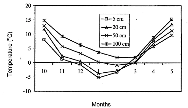
It is observed in the following Figure 3 that ground temperature is very much

dependent on the air temperature [7] . At -10°C to 10°C outside temperature, the

ground temperature is varying from-5°C to 8°C from months 1 to 5 for a depth of 5

cm. The variation at much greater depth of around 100 cm, the variation is ranging

o

20

-10

--10

-—B—Tair.min —&-Tair,max -X —Tair.mean

-20

30

--40

Months

Figure 2 Monthly variation of outdoor air temperature from October 2005 to May

2006 for Erzurm, Turkey

It is evident that the ground temperature very much depends on the outside air

temperature for certain depth [7]. . It is almost linear to the temperature outside

and is resilient for small changes.

o o 0 i_ 13 + —• CO i_ 0 Q. E 0

—B— 5 cm —Ar-20 cm —X— 50 cm H K -100 cm 15

-1 0

--10

Months

Figure 3 Monthly variation of mean ground temperatures at several depths from

Te

m

pe

ra

tu

re

(°

C)

As the depth increases, temperature increases and eventually stabilises around

constant value for greater depths and is no more affected by the outside air

temperature.

As the heat is absorbed from the ground, high thermal inertia of the ground

makes the temperature of the surrounding ground decrease very slowly. Before

the temperature further drops, energy from the surrounding ground is extracted.

This very nature of the ground makes it possible to use it as the infinite reservoir

for heat exchange.

Below Figure 4 shows the temperature of the ground is nearly constant after

certain depth the variations are shown from summer (August) and winter (January)

in Nicosia, Cyprus [8]. It is evident that earth temperature is nearly stabilised to a

constant value after certain depth irrespective of the geographical locations.

30 26 22 18

14 _25-Jan-05

20-Aug-05 10

6

0 5 10 15 20 25 30 35 40 45 50

Depth in ground (m)

1.2 Types of GSHP configurations

1.2.1 Open loop systems

In this system the water from the wells or ponds is used directly to add or reject

the heat to the primary loop heat exchanger in the system. The water from the

secondary loop is pumped back to the well or pond again. The cycle uses fresh

water each and every time it exchanges heat from the primary loop.

1.2.2 Closed loop system

In this system the secondary loop which carries the water or glycol exchanges the

heat with the source (water or ground) on one side and with primary loop on the

other side. The primary loop is the main system loop of the heat pump system

which involves compressor, condenser and evaporator and throttle valve. The

water in the secondary loop is re circulated.

1.2.2.1 Horizontal trenches (Closed loop)

Horizontal trenches are made for the pipes to be laid usually at 1-3m deep

underground. The area of the ground required depends on the heating capacity of

the building, but usually it is also dependent on the space availability and it

requires large area when compared to vertical borehole types. Below Figure 5

Figure 5 Horizontal closed loop heat pump system

1.2.2.2 Slinky coil horizontal system (Close loop)

Slinky coil system is another type of arrangement of horizontal loop systems, pipes

are laid in coil shape on the horizontal trench rather than the straight pipe. This

increases the surface area of the pipe for the given length of the trench laid hence

it increase the heat transfer process. The overlapped looped pipes can be 30 to

60% shorter than the traditional horizontal types and cheaper to install [9].

Following Figure 6 shows the general arrangement of the slinky coil system [9]

1.2.2.3 U- tube vertical boreholes (Closed loop)

On the other hand, vertical borehole type configurations are widely used because

of the space restrictions [4]. Vertical borehole types or the U-tube as they

generally called as require 30- 50% less tube length compared with horizontal

types for the same thermal loading, due to effect of high temperature at different

depths [10]. The borehole depths of up to 200m are being used for these types of

arrangements. Below Figure 7 shows the arrangement of vertical borehole system

[5]

Figure 7 Vertical U tube closed loop heat pump system

1.3 Cost comparison

The choice of different configuration is influenced by the cost associated with each

type. Following Figure 8 gives the capital costs for different configurations for

ground to water heat pump systems [11]. The investment on the coil for the

vertical system is more when compared to the horizontal system. On the other

hand it saves on the length of ground coil required for the same capacity as

System

Type Costs (£/KW)Ground coil Costs (£/KW)Heat pump Costs (£/KW)Total system

Horizontal 250-350 350-650 600-1000

Vertical

Indirect 450-600 350-650 800-1250

(Costs include installation and commissioning but exclude distribution system) Figure 8 Capital costs for different configurations

Direct exchange systems

It is the simple cycle in which the refrigerant from the heat pump is directly

circulated in the copper tubes buried in the ground. The heat is directly exchanged

between the refrigerant and the ground which in contrast to the secondary loop

containing water or antifreeze solution to exchange the heat with the indirect heat

pump system. This avoids the secondary loop; copper being good conductor of

heat, heat transfer rate is higher compared to the conventional pipes. It requires

copper tubes for greater length and more quantity of refrigerant for circulation

1.4 Typical Heat pump cycle operation

Room thermostat Heat pump and

circulating pump

Base board backup heat

Supply air

Return air

Heat Exchanger

Circulating pump

Ground loop

Figure 9 Typical Heat Pump Unit

GSHP system consists of three systems loops as shown in Figure 9 a ground

loop, a refrigerant loop, distribution loop and optional domestic hot water loop [5]

ground loop circulates the water in to the ground and extracts the heat, then enters

the refrigeration loop where it exchanges the heat with the refrigerant. The cooled

water will then enter the ground loop; hence the water keeps circulating in the

same loop. The refrigerant loop once getting heat from the ground water will

evaporate; the compressor then compresses the refrigerant vapour. The

compressed high temperature refrigerant enters the condenser and looses the

then expanded in the throttle valve before entering the evaporator. The heated

water in the distributed loop will be circulated in the building for heating purposes.

In cooling the building for summer conditions, the heat is absorbed by the cold

water in the distribution loop and transferred to the relatively cold refrigerant in the

evaporator. The evaporated refrigerants are then compressed in the compressor

and make its way to condenser to loose heat to the ground loop circulation water.

Warm water in the ground loop rejects the heat to the relatively cold surrounding

ground and it re-circulates again for the next cycle. The refrigerant after loosing

heat in the condenser, pass through expansion valve and enters the evaporator to

absorb heat from the distribution loop and this cycle repeats.

1.5 Role of GSHP in reducing C02 emissions

Properly sized and installed GSHPs have shown significant C02 reductions

compared to conventional fossil fuel boilers, in the UK context with the current

power station mix, 1kWh of electricity emits 0.43kg of C02[12]. At a Seasonal

Performance Factor (SPF) of 3.8, this can lead to overall C02 reductions in excess

of 40% compared to a ‘natural’ gas boiler. For gas grid, the C02 savings against

oil, LPG, coal or direct electric heating, the C02 emission savings are even higher

[6]. In the context of the Stern review, it is now interesting to ‘cost’ carbon savings.

Figure 10, extracted from a UK government report tabulates the relative costs and

outputs of different renewable energy technologies. The final row of the table

makes interesting reading for GSHPs. The existing capacity of the GSHPs is much

solar photovoltaic system is much higher than the ground source heat pump; it is a

clear choice for the other systems to be replaced with GSHP.

Over the last few years, GSHPs have gained significant popularity, especially in

the domestic market. Ease of maintenance and reasonable pay back period with

impressive savings of the energy bills makes it a more viable alternative than the

conventional systems.

Existing

Capacity Capital Cost£/kW kWh/yrper kW Pay back(years)

Saving Tonne C 02/yr Per

kW

Saving kgC/yr /E1000CAP

EX

Solar PV 8MW 6300 750 120 0.32 14

Micro-Wind - 2500-5000 1700 30 0.7 47

Solar Hot water

35MW 70,000

Installation 1250-2000 1000 80 0.2 54

GSHP 5MW 600_Units 1000-500 3000 15-20 0.4 91

(Source: UK DTI report-Renewable Heat and Heat from Combined Heat and Power Plants-2005) Figure 10 Comparison of several renewable energy techniques

Form Figures 10 & 11 significant reduction in C02 emissions can be achieved by

using GSHP systems. Figure 11 shows the relative fuel costs of the different

technologies, as well as the C02 savings. All heating and hot water supplied by the

heat pump, at an affordable cost, is a very satisfactory outcome. The table has to

be evaluated for each country and region to be relevant.

Annual fuel cost to run the GSHP system is very low compared to all the other

systems. The interesting fact remains that the emissions is the lowest among all

System Annual Fuel Costs Annual C 02 Emissions(tonnes)

GSHP £215 1.6

Natural Gas

(Condensing Boiler) £300 2.9

Natural Gas

(Non-Condensing) £345 3.3

Liquid Petroleum Gas

(Bulk-Non-Condensing) £500 4.3

Liquid Petroleum Gas

(Bottle-Non-Condensing) £670 4.3

Oil (35 sec) (Non-Condensing) £300 4.4

Direct Electric-Storage and Panels

With night time Low Cost Tariff £510 6.5

House Coal £380 6.6

Smokeless Coal £515 7.5

(House =10001^-12500KWh/yr as per SAP 2001)

Figure 11 Comparison of fuel costs and C02 emissions for GSHPs and fossil fuel

Boilers

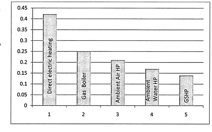
The following Figure 12 shows the Kg of C02 emissions for KW of energy

produced [13]. It is very clear from the table that GSHP is the lowest producer of

emissions compared to the other conventional and non-conventional methods of

heating .It is evident from the following figure that GSHP performs 50% better than

the ASHP. One more advantage being, the ground temperature is relatively

constant for all the seasons; hence the system can maintain its performance all

0.45 sz £ 0.4 0.35 CM

o

o

Heat source for building heating system

Figure 12 Comparison of carbon dioxides emissions from GSHPs and other forms

of heating

1.6 Methodology

Calculating annual building loads as well as long-term ground thermal response

for the demand, multi-year simulation is an invaluable tool in the design and

development of GSHP systems [14]. Predicting the performance of GSHP for

varying underground thermal properties, temperature and heating requirements

has been a difficult task. GHE operates with various dynamically operating

parameters, this gives an opportunity to study and improves its effectiveness, so

as to improve the performance of the whole system. It has to operate with varying

parameters such as load, soil temperature, configurations, thermal properties of

ground and soil condition. Since the pipe is buried in the ground, it is a difficult

task to calculate the thermal resistance between the borehole surface and pipe

external surface. The configuration of the pipe and deep ground characteristics

thermal resistance has been introduced by Kavanugh et al [15,16] in which a pipe

represented as a hollow cylinder with effective radius by assuming that the

external surface of the pipe is completely in contact with borehole surface.

The work of Eskilson [17] presents the methods based on non-dimensional

thermal responses for thermal interference between boreholes for multiple

borehole systems. These functions are computed numerically and the values are

given for various configurations of the pipes in the borehole. There have been a

number of models based on some analytical solutions suggested by Ingersoll [18]

and Hellstrom [19], but these models used oversimplified approaches to treat the

boreholes for short time behaviour. In many design programmes, the time of

interest is in the order of months or years. Boundary element method to calculate

thermal resistance in the grout has limited use for simple, straight-line flows, which

are practically not common. There are many programmes available for evaluation

of GSHP systems [20]; these tools only deal with a peak load and for simple or

basic heat exchangers.

This work is undertaken to develop a hybrid model combining analytical and

numerical solution techniques known as Computational Fluid Dynamics (CFD) to

predict the performance of GSHP and to identify the critical parameters, which

governs the COP of the heat pump by considering response of changes in the

load and the temperature difference between the room and the ground. The use of

CFD techniques in thermal analysis and turbulence modelling is widely gaining

Having gained much popularity, CFD deals with some limitations; it is difficult to

calculate the response for longer time of the ground and associated climatic

conditions. In order to deal with the climatic conditions over the year, a powerful

mathematical tool called MathCAD is used to develop the model of the borehole

along with the pipe. Performance evaluation is carried out for steady state

conditions by assuming the temperature on the outer surface of the grout as an

initial start. The simulations are also carried out for changing temperature of room,

ground, surface area of the grout and other varying parameters to observe the

effect on COP of the system.

From Fourier's law, heat conduction without the temperature gradient indicates the

material having no resistance to heat transfer or having infinite thermal

conductivity. Practically existence of these condition is clearly not possible,

however such condition is never be satisfied exactly. Such conditions can be

approximated, considering the resistance to the conduction within the solid is small

or negligible compared to the resistance to heat transfer between the solid and its

surroundings [22].

The temperature from the outer surface of the tube is modelled for Logarithmic

Mean Temperature Method (LMTD) for temperature distribution to the circulation

fluid. LMTD is the logarithmic average of the temperature difference between the

hot and cold sides of the fluid at each end of the exchanger. The larger the LMTD,

Incropera et al. [22] shows that the steady-state average fluid temperature is the

average log mean difference defined by LMTD.

ATm and AT0Ut are the fluid temperature variations, at the inlet and outlet,

with respect to the ground temperature (i.e. ATin = Tin - Tg) and Tg is the grout

temperature. This method is more accurate compared to the generally used

average temperature method which generally over predicts the temperature.

1.6.1 Use of CFD and MathCAD

The CFD model is used for calculating the overall thermal resistance of the

borehole by fixing the temperature on the surface of the grout. Previously the

attempts were made to calculate the thermal resistance of the borehole by using

Boundary Element Method (BEM) [20]. Here Finite Volume Method (FVM) does

the simulation. This method is more accurate since it integrates the residuals over

the entire domain before reaching the next iteration. This method converges

quickly and is more reliable compared to the boundary element method which

consumes both time and memory.

In this analysis, a 50 meter pipe is modelled with single u tube surrounding the

grout. The geometry and the properties of the complete system are obtained from

the manufacturer's handbook. Convergence is obtained for the values given in the

AT|m —I AT out| I AT in| (1)

published data; this model is used as a reference model for varying parameters.

The temperature on the surface of the grout is varied along the length to observe

the outlet temperature variations. To improve the model, different geometries and

material properties were suggested.

Each subsystem is represented by a set of equations and assembling each sub

systems represents the complete system. Simultaneous equations were solved in

MathCAD for the convergence and compared with the published data to validate

the model. The overall heat transfer coefficient from the CFD model is used to

verify the temperature variations and compared with published data, this represent

the complete system hybrid model.

1.7 Research objectives

To build the whole system model in MathCAD and use the operating conditions for

the model from the published data as input, to create a reference model. Once the

reference model is created the system is checked for the stability by changing

predefined variable and to look for change in the solution. If the unique solution

exists, the variables calculated will converge at the same value and with negligible

or no residuals.

Then the initial guess for the variables to be calculated is changed and checked

for the residue so that the convergence is achieved. This process gives the affect

values of material properties, flow rate, inlet water temperature to the GHE and

area of grout.

The results were analysed and the key parameter which affect the performance

are identified. The CFD model of the GHE is modelled and solved for the same

boundary conditions used for the MathCAD model to calculate the thermal

resistance of the GHE. The CFD results are analysed for temperature and velocity

distribution in water and temperature distribution in the grout material and pipe. It

also gives the surface heat transfer coefficient which can intern used to calculate

the thermal resistance. The results were analysed and discussed at the end and

necessary conclusions were drawn. Finally future scope for the model analysis is

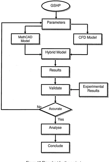
1.8 Block diagram of the project

GSHP

Parameters

MathCAD

Model CFD Model

Hybrid Model

Results

Experimental Results Validate

No _Accurate

Yes

Analyse

Conclude

Figure 13 Flow chart for the project

Above Figure 13 shows the steps followed to complete the cycle of the project.

The analytical model developed in MathCAD is compared with the experimental

created. The CFD model of the GHE gives additional information of the overall

heat transfer resistance of the heat exchanger. The final model is validated against

the published data. The results are discussed and the necessary assumptions are

made and discussed as appropriate.

Conclusion

The purpose of this first chapter has been to introduce the full scope of the project

and define the main objectives for such a study. It gives brief introduction about

the work to be carried out to build hybrid system. These remains centred upon

how ground heat has become important to study and evaluate as an important

Chapter 2

Introduction

The purpose to this section is to establish a working definition and framework for

the GSHP and its potential toward becoming a primary energy saving system. A

literature review acts a framework from which the analysis can be conducted and

continue towards further development of GSHP. Further exploration is needed in

order to build a foundation toward understanding new energy heat sources, which

may work better toward ‘green’ initiatives. Methodologies use do model ground,

thermal loading and environmental variables which affects the ground thermal

storage, developed by different authors has been discussed. Building hybrid model

in MathCAD and CFD has been outlined. Assumptions made for the modelling and

its limitation due to complex working nature have also been discussed.

2.1 Literature Review

Until 1980's not much significance was given to the ground thermal storage

systems. Growing demand for the green energy initiative has given significant rise,

since then much work is done in geothermal energy extraction techniques.

One of the projects such as Metropolitan housing trust head quarters in

Nottingham, UK has invested in greener energy initiatives. Major research work

and development of GSHP technology with innovative applications such as hybrid

GSHP systems and development of environmentally-friendly refrigerants are being

carried out across many universities in the UK [23, 24]. The major deriving force in

commercial market to strengthen GSHP's competitiveness at the global level [25].

Countries such as US, Canada, China, South Korea installed and successfully

operating the GSHP systems for industrials and domestic applications.

A geothermal heat pump can transfer heat stored in the earth into a building during

the winter, and vice versa during the summer. GSHPs are increasingly becoming

popular due to their reduced primary energy consumption and there by reducing

emissions of greenhouse gases. The technology is well established and adopted

in USA and Europe.

A typical heat pump require 100kWh of power input to turn 200kWh of freely

available environmental or waste heat into 300kWh of useful energy [26]. This

saving of 200kWh correspondingly reduces the emissions of harmful gases such

as carbon dioxide (C02), Nitrogen oxides (NOx) and Sulphur dioxide (S02).

Approximately the total number of globally installed GSHP-systems sums up to

about 12,000 MWth[27]. This as almost equalling to the total number of global

systems estimated around 1,100,000 units, of all the GHE types available, it was

found that vertical closed loop type contribute to 46% of the systems and

horizontal closed loop type contribute to 38% in USA alone, while the remaining

are open loop systems [28]. In the last two to three decades, significant research

has gone in to relating the effect of properties of ground, pipe and grout material

on the performance of the GHE system. The goal being optimisation of the heat

transfer mechanism and installation method used for the given ground type.

thermal power is 50-80 W/m. For vertical GHE's one or two U tubes per bore hole

is the most commonly used configurations. The sizing of the GHE depends on the

load, thermal and physical properties of the soil such as thermal diffusivity,

density, specific heat capacity, thermal conductivity, etc. Thermal conductivity of

the tubing, grout material and the ground temperature plays important lone in

designing of the GHE system. For typical ground conditions, Pahud and Matthey

[30] suggest 50 W/m thermal power to be considered in designing a GHE, with

ASHRAE [31] as also confirming around the same value. Taking into account,

however; the parameters such as:

• The thermal loading on the building is not a steady state condition

• The time required by the GHE to reach steady state condition is

comparatively longer due to its high thermal inertia. It is estimated around

30 tonnes of soil per m2 of building area is required for heating and cooling

operations.

• System is used alternatively for both heating and cooling purposes, it is

important to consider the energy sustainability in the ground in response to

the change in working nature of the heat pump system.

The critical parameter in designing the vertical system is the thermal power per

meter of borehole that the GHE can handle [32]. With this mind, it is important to

2.1.1 Coefficient of Performance (COP)

According to the first law of thermodynamics, in a reversible system we can show

that

Qhot — Qcold "I" W (2)

and

W — Qhot" Qcold (3)

Where

Qhot = heat given off by the heat reservoir (Watts)

Qcoid = heat taken in by the cold heat reservoir (Watts)

W= Work input (Watts)

Therefore, substituting for W from the definition of COP,

For a heat pump operating at maximum theoretical efficiency (i.e. Carnot

efficiency) it can be shown that

COP heating — Q hot (4)

Q hot ” Q cold

Q hot _ Q cold

T hot Tcold (5)

and

(6)

Thot = Temperature of the hot reservoir (°K)

Tcoid = Temperature of the cold reservoir (°K)

Hence, at maximum theoretical efficiency,

C O P heating — T hot (7)

Similarly, for cooling

P O P _ ^ c0^ _ co*^ / o \

o U r cooling — n n —T T (o;

W hot" W cold I hot I cold

It can also be shown that COP COoiing = COP heating - 1.

Note that these equations must use the absolute temperature, such as the Kelvin

scale. COP heating applies to heat pumps and C O P COoiing applies to air conditioners

or refrigerators.

Although COP can never be remotely approached in practice to the theoretical

values, it is useful as a reference to indicate important influencing factors. It is

evident that the COP increases as the temperature difference between the

condenser and the evaporator decreases.

The COP system can be calculated from the following equation

system

pumps (9)

Where,

COPSystem =COP of the whole system

WpUmps = Work input to the circulating pumps (Watts)

Wfan = Work input to the fans (Watts)

W^ = Work input to compressor (Watts)

For engines, efficiency is the general term in use for which values for actual

systems will always be less than these theoretical maximums.

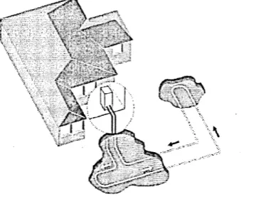
2.1.2 Ground Heat Exchanger (U tubes)

Vertical ground loop exchanger typically consists of High Density Polyethylene

(HDPE) pipe U-tube as shown in Figure 14 inserted in to 50 meter deep vertical

borehole drilled in the ground [33]. The borehole has a diameter of 150mm and a

polyethylene pipe of 32mm internal diameter with 4mm thickness is used to

circulate the water for the ground circuit. Circulating water in the pipe absorbs the

heat from the refrigerant in the heat pump and rejects the heat to the ground on

the other side or vice versa

Ground 'surface Fluid

Fluid inlet

Utube Grout .Borehole

■Ground ,Far field

boundary

Once the U-tube is inserted in to the borehole, the rest of the gap between the U-

tube and the borehole is filled with grout mixture. The very purpose of the grout

being used is to improve the heat transfer between the soil and plastic pipes by

providing a better contact surface and also to provide a seal around the U-tube to

prevent against the contamination in the ground water system. For this very

reason, the maintenance is nearly zero for such systems.

2.1.2.1 Configurations of ground tubes

There are basic configurations which are generally used are shown in 15 & 16 [8]

Single U pipe Double U-Pipe

Pipe diameter = 25-32 mm Pipe diameter = 25-32 mm

Width 50-70 mm Max. Width= 70-80 mm

Figure 15 Basic configurations of Vertical U tubes

Simple Coaxial ~ ~ ,

External Diameter = 40-60 mm .. _{Max. Width = 70-90mm}vrfon

The ground heat exchanger is the closed vertical type (U-shaped) and generally

has 24-30 boreholes of depth ranging from 50- 175 m in depth depending on the

load requirement. The distance between the boreholes generally maintained

around 5 m. Thermocouples measures subterranean temperatures in the ground

located at 1.5 m and 2.5 m away from the outer surface of the heat exchanger.

Ground temperature might be varied with the temperature of the ground heat

exchanger [34]. Ground temperature distribution may vary with different surface

cover (such as bare ground, lawn, and snow), two different locations for example,

bare land and grass lawn has been selected to measure the temperature

distribution in the ground at different depths [35]. Cu-Konstantan thermocouple

wires and thermocouple meters SR60 (Stanford Research System, USA) were

used by POPIEL et al [36] to measure the temperature at different time intervals.

Survey suggest that because of the complexity of acquiring the physical properties

of ground and surface boundary conditions, simple empirical formulas such as for

example formula proposed by Baggs [37,38] is commonly used.

For studying the heat transfer phenomena in transient condition most models uses

step response for the heat transfer rate. Superimposing principle allows the final

solution to be the form of convolution of these individual step contributions [39].

2.1.2.2 Effect of air temperature ground circulating water

Figure 17 shows evolution of daily averaged subterranean temperature at the

depth range from 2.5-30 m and outdoor temperature measured during March 21-

September 30, 2007 [34]. The ground is influenced by the outdoor air temperature

temperature of the ground was observed to keep constant around 16°C regardless

of the abrupt change in the outdoor temperature

CL _{Outdoor temp.}

Ground temp. (2.5m) Ground temp. (5m) Ground temp. (10m)

Ground temp. (20m) Ground temp. (30m) 10

3/21 4/13 5/06 6/08 7/05 7/30 9/02 9/23

Date (Month/Day)

Figure 17 Evolution of daily average subterranean temperature and outdoor air

temperature

Figure 18 shows the outside air temperature, average temperature of circulating

water, the surface temperature of the ground heat exchanger at 1.5 m and 2.5 m

away from the ground heat exchanger at the depth of 10 m [34].

As the outdoor temperature increased, the temperature of circulating water was

increased up to 22 °C. This gives the indication that the cooling load increased as

30

Q .

— Outdoor temp. — Circulating water temp.

GHEX surface temp.

Ground temp. (1.5m) from GHEX Ground temp. (2.5m) from GHEX I U

3/21 4/13 5/06 6/08 7/05 7/30 9/02 9/23

Date (Month/Day)

Figure 18 Evolution of daily average temperatures of outdoor air, circulating water,

surface of ground heat exchanger

It can be seen that the temperature of circulating water strongly affected the

surface temperature of the ground heat exchanger. The temperature of the ground

appeared to be constant regardless of circulating water temperature at 1.5 m and

2.5 m away from the surface of the heat exchanger.

2.1.3 Condenser and evaporator

The heat balance and the heat exchange from the water circulating in the pipe is

analysed in the water to refrigerant heat exchanger at the condenser side of the

heat pump. Plated Heat Exchanger (PHE) is assumed to be used in the

calculation. Plated heat exchangers are the natural choice for flexible chillers and

climate control applications for its high effectiveness, versatility and ease of

half load. PHE is mainly made of thin, corrugated alloy plates held in a carbon

steel frame, each plate is separated by a gasket to avoid leakage. Plates are

arranged in a manner to make flow channels by the arrangement of the gasket

pattern and the ports of each corner of the plate acts as a header for the main flow

line.

It has a major advantage over a conventional heat exchanger in that the liquids

spread out over the plate. This facilitates the transfer of Heat, and greatly

increases the speed of the temperature change. In a PHE plates are generally

arranged in such a way that it forms channels of hot and cold liquid alternately.

Due to corrugations in the plate, high turbulent flow increases the heat transfer

rate.

As compared to Shell & Tube heat exchanger, for the same amount of heat

exchange the size of the PHE is small, because of the large heat transfer area

afforded by the plates. Expansion of the heat transfer area is possible in PHE just

by adding the number of corrugated plates. These types of heat exchangers are

widely used in district heating and cooling especially where the heat transfers

between two-phase liquids. Since the refrigerant in the condenser is partial mixture

Inspection cover Roller assembly

Support Column Plate pack

Carrying bar

Support foot/ Guide bar Tightening nut

Lock washer

Tightening bolt

Movable cover

Bearing Box Shourd

stud bolt

Fixed cover

Frame foot

Figure 19 Typical Plate Heat Exchanger

Above Figure 19 gives the arrangement of the heat transfer between the warm

water and relatively hot refrigerant or vice versa in case of evaporator [40]. Heat

transfer in the condenser and evaporator occurs at phase change of the

refrigerant; hence the temperature of the refrigerant is constant (latent heat

transfer). The amount of heat transfer is calculated by taking the enthalpy change

with the mass flow rate of the refrigerant.

2.1.4 Methodologies used to model the Heat Pump System

The equations developed earlier to represent the heat pump are based on the

assumption of one-dimensional flow, which were replaced by two-dimensional

models during the 1990s and three-dimensional systems during recent years.

Models have been devised in three dimensions but it seems one-dimensional

extensively used to take account of thermal conductivity and heat flow in the

ground surrounding the grout.

Borehole thermal resistance bears strong impact on the GHE performance. This is

defined by the thermal properties of the construction material used and the

arrangement of flow channel of the water pipes in the ground. The common

methods for heat transfer in the semi-infinite medium from a perpendicular buried

infinite cylinder were the cylindrical source and the line source solutions. While the

cylindrical source solutions assume steady heat flux on the boundary of the

borehole into the surrounding medium, the line source solution is based on the

steady release of the heat of constant strength through an infinite line [40].

The thermodynamic analysis for the performance characteristics of the GSHP

systems with U-tube ground heat exchanger for heating can be considered with

mass, energy, entropy and exergy balance relations. It has been shown that the

performance can be evaluated by energetic and exergetic aspects [41]. In

thermodynamic analysis of energy systems, exergy analysis is proven to be a

powerful tool .Exergy is calculated by setting a reference environment. It is used to

detect and quantitatively evaluate the cause for the thermodynamic imperfection in

the thermodynamic process. But only an economic analysis can decide the

expediency of a possible improvement. The results of the exercise shows that the

uncertainty analysis needed to prove the accuracy of the experiments

[42].According to Kavanaugh and Rafferty [43] energy performance of the system

is also influenced by the pumping energy required to circulate the fluid through the

Rafferty [43] suggested the guidelines for pumping power for commercial GSHP

systems. The values shown in Figure 20 is proposed as a benchmark for

measuring the effectiveness of a pumping efficiency and piping system design for

a minimum of 0.162m3/h per KW of cooling, with optimum pumping flow rates

ranging from 0.162 to 0.192m3 /h per KW of cooling [44].

Watts Input Performance

Efficiency Grade

Per Tonne Per KW

<50 <14 Efficient Systems A:excellent

50-75 14-21 Acceptable systems B:good

75-100 21-28 Acceptable systems C:medium

100-150 28-42 Inefficient Systems D: poor

> 150 >42 Inefficient Systems E:bad

Figure 20 GSHP System pumping efficiently required pumping water to cooling

capacity

2.1.4.1 Ground temperature variation modelling

Determining the temperature in the ground is a transient and complicated process.

Over the past few years significant work has been done to develop algorithms to

simulate the temperature inside the ground surrounding the pipe and heat carrier

fluid in GHE. Developed algorithms should be tested against the experimental

work to validate the calculation results. Reports are available relating to the

comparisons made for various other simulation models [45]. Several field

Below 21 shows the earth temperature is nearly constant far away from the outer

surface of the pipe [48] Solar assisted GSHP is operated alternatively for a period

24 h with and without solar power for an interval of 4 hours of operation. The effect

of the solar assist on the temperature distribution around the pipe is negligible.

The ground seems to be more resilient in temperature for loading and unloading

conditions. 14 12 10 -8 -6 - 4-2 - 0--2 -0. O o CD 3 c5 (5 Q . E 0 •c_CO L it

- m — Z -1m

• — z=3m a —z=5m r —z=7m

z=9m

< — z=11m

►—z=13m

— 0— 7 = 15m

0 0.2 0.4 0.6 0.8 1.0

Radius (m)

Figure 21 Earth temperature distribution surrounding buried coil at different depth

after 4 hour operation of GSHP

Below figure 22 shows the temperature of the earth decreases near the outer

surface of GHE as the operation time increases and seems not affected at far

distance [48]. Its give the clear idea that because its thermal inertia, system should

■e_aJ

LU 4 _{4 8 12 16 20 24 28 32 36}t— i— |— i— |— r— |— i— |— i— |— i— r

—■— r=0.05m

— r=0.15m

— r=0.25m

— r=0.45m

— r=0.65m —« _ r=0.85m

— r=1.00m

Operation time (hours)

Figure 22 Earth temperature variation with the operation time of GSHP at a depth

of 5 m for different radius

Investigation on narrow channel models is becoming more important lately.

Research work on wide diameter ratios was carried out at significant levels. It is

observed that heat transfer characteristics of narrow annuli are different from

conventional channels. Measurements were carried out for heat transfer

coefficients in a narrow channel for a mercury flow [49]. Experiments conducted to

calculate heat transfer coefficient at the inner wall of concentric annuli with wide

diameter ratios for turbulent flow was suggested [50] It can also be seen that the

choice of diameter ratio has an effect on the convective heat transfer coefficient.

The Finite Element Model (FEM) developed to simulate natural convection and

heat transfer around the annulus is interesting to observe how parameters such as

flow rate and temperature can affect the heat transfer coefficient [51]. It is shown

that the extended algebraic turbulence model is important for predicting flow

On the basis of works conducted before, it can be observed that there is an affect

on the heat transfer mechanism on the geometry of the pipe

2.1.4.2 Thermal loading on the borehole

Simulation conducted by C K LEE et al [53] shows the importance of loading on

the performance of the system in which loading is done on the borehole with

temperature profile for steady state condition. The temperature in the ground and

temperature profile on the borehole is greatly influenced by the initial loading

temperature profile. Figure 23 shows with constant load for single borehole,

neither of the borehole temperature and borehole loading was constant along the

length of the borehole. This shows that the single finite difference scheme is not

sufficient to estimate the performance by superposition.

Borehole temperature rise (°K)

6 7 8 9 10 11

0.2 ■©—- 2 years

■A— 5 years - X— 10 years

X 0-4

N 0.6

Figure 23 The borehole temperature rise profiles at different times

Where,

d= depth of borehole top from ground surface (m)

H= length of borehole (m)

It is evident that the temperature raise is very little over the years. At least for 10

years it shows that the system is very resilient.

Borehole loading (W/m)

30 35 40 45 50 55 60

0.2

-El— 2 years -A— 5 years

X— 10 years

5 0.4

■o

0.6

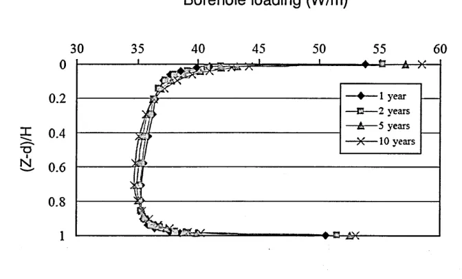
Figure 24 Borehole loading profile against a dimensionless parameter (z-d/H) (with

value one at bottom and zero at borehole top)

From Figure 24 it was found that neither the temperature nor the loading was

constant along the borehole. Borehole temperature is maximum at the top if finite

line source model is used. Then the loading is decreased till bottom end this could

be assumed that the mean fluid temperature inside the borehole decreased with

depth.

By assuming no thermal resistance between tube and surrounding soil, the heat

flux can be calculated by temperature difference between inlet and outlet of GHE

and mass flow rate of heat carrier fluid. Figure 25 shows considering convective