A Comparison of Supervised Learning Algorithms for the Income Classification

A Comparison of Supervised Learning Algorithms for

the Income Classification

Mohammed Temraz

Dublin Institute of Technology, Ireland

ABSTRACT

The fundamental population data are needed for every country for purposes of planning, development, and improvement. Census data can provide the basic population data of any country. Moreover, they are rich with lots of hidden information that can be used for machine learning and data mining tasks in order to provide services for country's social and economic development. This paper is focused on the applications of data mining and machine learning in census data to classify the annual income. It aims to show a systematic comparison to examine and evaluate three supervised learning classifiers. The classifiers that have been targeted are decision trees, random forests, and artificial neural networks. The main aims are to explore not only the classifiers properties and the impact of the attributes on the evaluation, but also, evaluate their classification performance under certain conditions to understand how the performance of the models changes over different experiments which potentially provide a guidance to help researchers to determine the most suitable classifier in census data.

General Terms

DT, RF, ANN

Keywords

Census Data, Data Mining, Classification, Supervised Learning, Decision Trees, Random Forests, Artificial Neural Networks, Performance Metrics.

1.

INTRODUCTION

The growth of the information technology sector has led to collect a huge amount of data in several fields, ranging from health care sector, telecommunication, finance, retail to banking, media and entertainment. However, the data collected may not reflect useful information and knowledge. In order to improve the decision-making process, the data collected need to be analyzed with a clear approach to extract the useful knowledge from it. Census is another important source of data. It is the process of gathering information about the citizens of a given country. It can be a combination of economic, social and other data. Census data can be represented visually or analyzed in complex statistical models, to show the difference between certain areas, or to understand the association between different personal characteristics. In recent years, data mining and its association technologies have become one of the crucial elements of any organization that collect the data. This is because that data mining plays a key role in the decision-making process. Moreover, in recent years, many researchers’ aim to build systems and develop algorithms that can automatically learn from data to gain knowledge from experience, and to gradually improve their learning behavior. Data mining is also becoming increasingly significant in the processing of census data. It is crucial that an appropriate algorithm be used as it has an impact on the results and knowledge derived [1]. This paper will use the

census dataset from the United States Census bureau and the task is to predict whether a given individual makes over $50,000 a year.

2.

LITERATURE REVIEW

3.

METHODOLGY

A quantitative approach is used to classify features and constructing statistical models and figures to explain what is observed. The dataset is already available from UCI Machine Learning Repository and it has already been extracted by Barry Becker and will be passed through the statistical process.

3.1

Data Description

The data set provided consists of 15 variables (9 nominal and 6 continuous), and 48,842 observations. The target variable is “Annual Income”, and it is a dependent variable. The other variables are independent. The income is divided into two classes: <=50K and >50K (Binary classification problem). The nominal variables are Work Class, Education, Marital Status, Occupation, Relationship, Race, Annual Income, Native Country, and sex. In contrast, the continuous variables are Age, Capital Gain, Capital Loss, Fnlwgt, Hours per week, and Education Number.

Table 1: A Summary of the Census Dataset

Statistics Numbers

Total dataset size 48,842 instances

Number of features 15

Nominal 9

Continuous 6

3.2

Preprocessing

The Pre-processing step is often the most critical elements determining the effectiveness of real-life data mining applications [2]. There are several data pre-processing techniques. Data cleaning techniques can be applied to remove noise, fill in missing values and correct inconsistencies in the data [9]. Data transformations, such as normalization, is also applied. Pre-processing is an aspect of data mining of which the importance should not be underestimated. If this phase is not performed it is not possible for the mining algorithms to provide reliable results [2]. A number of preprocessing steps was taken place before building the classification models, such as filling in missing values, transforming the input variables that are not normally distributed.

3.2.1

Missing Values

Missing values are a common occurrence in real data sets. They are frequently indicated by out-of- range entries. Many of the values are unknown or missing, as indicated by question marks. For nominal attributes, missing values may be indicated by blanks, dashes or question marks [10]. The dataset used in this paper had a missing values rate as 13.23%. These values are indicated by question marks. Table 2 shows a summary of the missing values. When building the classification models, it is crucial for some models to replace (fill in) values for observations that have missing values. As the variables that have missing values are class variables, they are replaced by the most frequent value for that variable. As a result, a new variable is created for each variable for which missing values are imputed. It has the same name as the original variable but is prefaced with IMP_. The original version of each variable exists in the exported data and has the role Rejected.

Table 2: Missing Values Statistics

Input variable Missing values Count percentage

Occupation

2809 5.75%

Work Class

2799 5.73%

Native Country

857 1.75%

3.2.2

Transformation

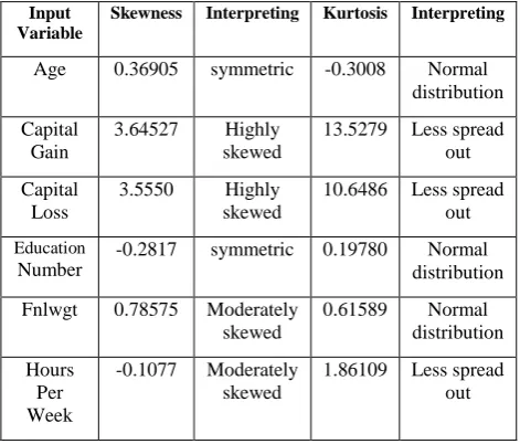
For some algorithms such as neural networks, transforming input data can lead to better model fit. This transformation can be a function of one or more variables. Variables whose distributions are not normally distributed, will be transformed in order to be used for neural networks models. Two variables, Capital_Gain and Capital_Loss have right skewed distribution and are less spread out (Table 3). They are transformed using “Log 10” transformation method which is used to control skewness. These variables will be transformed by taking the logarithm with base 10 of the variable. This can be valuable for making patterns in the data more interpretable.

Table 3: Skewness and Kurtosis Statistics

Input Variable

Skewness Interpreting Kurtosis Interpreting

Age 0.36905 symmetric -0.3008 Normal distribution

Capital Gain

3.64527 Highly skewed

13.5279 Less spread out

Capital Loss

3.5550 Highly skewed

10.6486 Less spread out

Education

Number

-0.2817 symmetric 0.19780 Normal distribution

Fnlwgt 0.78575 Moderately skewed

0.61589 Normal distribution

Hours Per Week

-0.1077 Moderately skewed

1.86109 Less spread out

3.2.3

Variable Selection

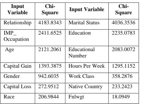
The variable selection method is used to identify input variables that are useful for predicting the target variable. For the classification model with the categorical target, chi-square test is selected. The chi-square test of independence is used to test for a statistically significant and is always computed for categorical variables. It is possible to generate chi-square statistics for interval variables by binning the type of variables. The default is 5 bins. So, interval variables are distributed into five bins and chi-square statistics is computed for the binned variables.

Educational_Number come next. In contrast, there are some variables that does not affect the classification models because they have low chi-square, such as race, native country and Fnlwgt. These variables will not be considered in some of the models.

Table 4: Chi-square Statistics

Input Variable

Chi-Square Input Variable

Chi-Square

Relationship 4183.8343 Marital Status 4036.3536

IMP_ Occupation

2411.6525 Education 2235.0783

Age 2121.2061 Educational Number

2083.0072

Capital Gain 1393.3875 Hours Per Week 1295.1152

Gender 942.6035 Work Class 358.2876

Capital Loss 272.9512 Native Country 233.2423

Race 206.9844 Fnlwgt 18.0949

3.3

Re-sampling

Imbalanced data refers to a problem with classification tasks where the classes are not represented equally. In this paper, the target variable has a 2-class (binary) classification problem with 48,842 instances. A total of 37,155 instances (which represent 76.07% of the dataset) are labelled with income less than 50K, and the remaining 11,687 instances (which represent 23.93% of the dataset) are labelled with income over 50K. This is an imbalanced dataset and the ratio of the two classes is 76:23. As a result, this might affect the performance of the training set and the prediction of the result from each classifier. In order to tackle the imbalanced data problem, under-sampling technique was used before creating the predictive models. Under-sampling is a technique used to adjust the class distribution of a data set. It was used to reduce the majority class so that income less than 50K would represent 40.0007% of the dataset, and income more than 50K would represent 59.9993% of the dataset. This approach helped to improve run time and storage problems by reducing the number of training data samples. One disadvantage of this technique is that it may affect the performance of classification models, because it may discard useful information which could be important for building the models. But, under-sampling technique was used because it helps to decrease the likelihood of overfitting since over-sampling technique will replicate the minority class events and add copies of instances. As a result, the experiments for classification were carried out using the 29,217 instances from the dataset, 11,687 instances for the income more than 50K and 17,530 instances for income less than 50K will be used.

4.

CLASSIFICATION MODELS

EXPERIMENTS

In this section, 27 classification models’ experiments will be designed and trained using different settings to predict the annual income. The experiments will be divided into three main groups, each group consists of nine experiments for a specific classifier.

4.1

Decision Tree Experiments

Decision trees (DT) are one of the most common machine learning methods used for data mining [2]. DT classification is the learning of decision trees from class-labelled training tuples, and is a flowchart like tree structures, where each internal node (non-leaf node) denotes a test on an attribute, each branch represents an outcome of the test, and each leaf node (or terminal node) holds a class label. The topmost node in a tree is the root node [9]. DT was also found to be able to handle large scale problems due to its computational efficiency, provide interpretable results and in particular, able to identify the most representative attributes for a given task. They are especially attractive in data mining environments since human analysts readily comprehend the resulting models [2]. For DT experiments, nine proposed versions of decision trees are created and trained under different conditions (Table 5).

Table 5: Decision Tree Experiments

Models Number of splits No. of depth Leaf size

DT1

2 splits (default)

6 (default) 5 (default)

DT2 6 220

DT3

3 splits (default)

6 5

DT4 6 220

DT5

5 splits (default)

6 5

DT6 6 220

DT7 A Tree with 6 features and 2 splits

DT8 A Tree with 6 features and 5 splits

DT9 A tree with binning “age” and transforming

skewed variables

4.2

Random Forest Experiments

A random forest (RF) is an ensemble training algorithm that constructs multiple decision trees. It suppresses over- fitting to the training samples by random selection of training samples for tree construction in the same way as is done in bagging [11]. In a RF, the features are randomly selected in each decision split. The correlation between trees is reduced by randomly selecting the features which improves the prediction power and results in higher efficiency [12]. RF algorithm works by minimizing correlation while maintaining strength. It is achieved by injecting the randomness into the training process. Particularly, random selection of features results in diverse learners which are still individually strong due to splitting using the best feature from the random fraction [13]. There are two key parameters to tune the RF: The maximum number of trees, and number of variables to consider in split search. RF will be examined under certain conditions depending on these parameters. Nine versions of the RFs will be investigated and trained (Table 6).

Table 6: Random Forest Experiments

Number of trees Number of variables

RF1 50 4 (default)

RF2 50 7 (50%)

RF3 50 All variables (100%)

RF4 100 4

RF5 100 7

RF6 100 All variables

RF7 300 4

RF8 300 7

RF9 300 All variables

4.3

Neural Networks Experiments

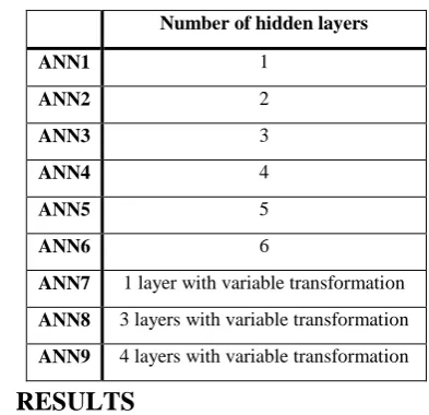
Artificial Neural Networks (ANN) are one of the data mining techniques, which have an interesting history in the annals of computer science [14]. In the past decade, ANNs have emerged as a technology with a great promise for identifying and modelling data patterns that are not easily discernible by traditional statistical methods [15]. ANN are a class of parametric models that can handle a wider variety of nonlinear relationships between a set of predictions and a target variable. Generally, an ANN is a set of connected input/output units in which each connection has a weight associated with it. During the learning phase, the network learns by adjusting the weights so as to be able to predict the correct class label of the input tuples [9]. Nine different proposed versions of the ANN will be investigated and trained using different number of hidden layers in order to determine the optimal number of hidden layers to predict the annual income (Table 7).

Table 7: Artificial Neural Networks Experiments

Number of hidden layers

ANN1 1

ANN2 2

ANN3 3

ANN4 4

ANN5 5

ANN6 6

ANN7 1 layer with variable transformation

ANN8 3 layers with variable transformation

ANN9 4 layers with variable transformation

5.

RESULTS

This section aims to present an evaluation of twenty-seven classification models results. Each model was trained under different settings in order to discover the model that gives the best result for the prediction of the annual income. Nine models were trained for the decision trees algorithm, nine models were trained for the random forest algorithm, and nine models for the neural networks’ algorithm. This section aims to analyze the results obtained from the implementation of the experiments and evaluate the performance of classification

models to determine which model is the most suitable in census data. Therefore, the evaluation will be completed on all the classification models and showing a systematic comparison to discover and examine the performance of each predictive model in census data. Evaluating model performance with the data used for training is not acceptable because it can easily generate overfitted models. So, the performance of the classification models will be evaluated on the validation data. As a binary classification problem, accuracy, misclassification rate, specificity, precision and recall will be computed from a confusion matrix for a binary classifier.

Figure 1: What is the Best Model?

5.1

Decision Tree Results

5.1.1

Accuracy and misclassification rate

It is desirable to begin by running the model on default parameters to get a baseline. Model DT1 is the decision tree on default parameters with 2 splits, 6 depths, and 5 leaves. This model starts off with 81.10% accuracy on the training. Min-sample-per-leaf node was set and increased to 220 in the second model, which means the tree will stop growing early. Accuracy did not see an improvement, and it decreased to 81.05%.

Number of random splits per node was set to 3 splits in model DT3 and DT4. Accuracy saw an improvement. The accuracy increased to 82.79% in the model DT3, and to 81.99% in model DT4 on the validation.

The models DT5 and DT6 are built with 5 splits using default parameter for maximum depth size and minimum leaf size, and then changing the leaf size to 220. In the DT5 model, the accuracy saw an improvement compared to the accuracy of two split decision tree. But in the DT6 model, the accuracy decreased to 80.46% on the validation data, which means that increasing the split size to 5 splits and leaf size to 220 are not preferred.

The DT7 and DT8 models were trained using feature selection method, where only the best six features (Independent Variables) have been given a chance to participate in becoming a decision node. The six features that have been chosen are relationship, capital gain, occupation, educational number, age, and hours per week. They have been chosen because they had the highest importance value. These models were trained to determine whether removing some independent variables can improve the accuracy of predictive model. As a result, accuracy has decreased slightly against a baseline, with only 80.96%., and did not see a great improvement. This is may be due to that the number of predictor variables was small. So, applying features selection as a method that can increase model accuracy is not suitable for a small number of predictors.

The last model was trained by pre-processing the data (transforming skewed variables). The performance of the DT

The Best Model?

Neural Networks

Models Random

Forest Models

was not improved by pre-processing the data, where normalization had no impact on the performance of a decision tree. So, this procedure would not help to affect the performance of the model.

5.1.2

Sensitivity and Specificity

Sensitivity (Recall) and specificity are other statistical measures of the performance of a binary classification test. DT classifier has reached its optimum specificity of 85.62% using 5 splits (model DT6). In overall, DT classifier showed a stable overall performance with 82% of sensitivity, specificity and accuracy using default settings with 3 splits (Model DT3).

5.1.3

The Best Model

A decision tree with 3 splits, and 5 leaf size (model DT3) was the best model which achieved 17.20% in misclassification rate, 82.79% in accuracy, 0.7634 in precision, 0.8296 in Specificity, and 0.8253 in recall. This model represents the best model in the decision trees experiments.

Figure 2: DT Results

Table 8: The Results of Decision Tree Experiments

MISC% ACC% Precision SPC Recall

DT1 18.89 81.10 0.746 0.818 0.799

DT2 18.94 81.05 0.724 0.785 0.848

DT3 17.20 82.79 0.763 0.829 0.825

DT4 18.00 81.99 0.764 0.837 0.793

DT5 17.29 82.70 0.768 0.836 0.812

DT6 19.53 80.46 0.771 0.856 0.727

DT7 19.03 80.96 0.744 0.817 0.797

DT8 17.80 82.19 0.778 0.852 0.776

DT9 18.66 81.33 0.742 0.811 0.815

5.2

Random Forests Results

For random forests experiments, nine proposed versions are created and trained using 50 trees, 100 trees, and 300 trees, with 4 variables, 7 variables, and 14 variables. The performance of random forests classification models will be assessed based on two important parameters including the number of trees, and the number of selected features to consider in split Search.

5.2.1

Evaluation of RF against the number of

trees

The first step was aimed to evaluate and investigate the performance of RF against the number of trees. In order to achieve this goal, different numbers of trees were randomly selected to be trained, including 50 trees, 100 trees, and 300 trees. The first model was created using 50 trees and 4 variables, and it started off with 82.99% accuracy on the validation set. Model RF2 was created using 50 trees and 7

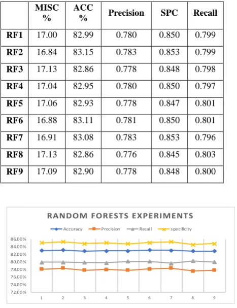
variables, accuracy has increased to 83.15%. Models RF4, RF5, and RF6 are created using 100 trees, the accuracy has slightly decreased compare to 50 trees. Models RF7, RF8, and RF9 are created using 300 trees, accuracy did not also see a great improvement. As a result, random forests classifier works well when the number of trees was 50.

5.2.2

Evaluation of RF against the number of

features in split search

The second step was aimed to evaluate and investigate the performance of RF against the number of features to consider in split search. In order to achieve this goal, different numbers of features were randomly selected to be trained, including 4 features, 7 features (which represents 50% of all features), and all features (100%). The experiment results show that there is no significant effect for random forest classification performance when increasing the number of randomly selected features. This is because the number of features in the census dataset is small. However, selecting 50% of the total number of features (7 features) achieved the best result, with 83.15%.

5.2.3

The Best Model

Among the nine models trained for RFs, a random forest with 50 trees size, and 7 variables (model RF2) was the best model which achieved 16.84% in misclassification rate, 83.15% in accuracy, 0.7838 in precision, 0.8532 in specificity, and 0.7990 in recall.

Table 9: The Results of Random Forest Experiments

MISC %

ACC

% Precision SPC Recall

RF1 17.00 82.99 0.780 0.850 0.799

RF2 16.84 83.15 0.783 0.853 0.799

RF3 17.13 82.86 0.778 0.848 0.798

RF4 17.04 82.95 0.780 0.850 0.797

RF5 17.06 82.93 0.778 0.847 0.801

RF6 16.88 83.11 0.781 0.850 0.801

RF7 16.91 83.08 0.783 0.853 0.796

RF8 17.13 82.86 0.776 0.845 0.803

RF9 17.09 82.90 0.778 0.848 0.800

Figure 3: RF Results

65.00% 70.00% 75.00% 80.00% 85.00% 90.00%

1 2 3 4 5 6 7 8 9

D EC I S I O N T R E E EX P E R I M E N TS

Accuracy Precision Recal l specificity

72.00% 74.00% 76.00% 78.00% 80.00% 82.00% 84.00% 86.00%

1 2 3 4 5 6 7 8 9

RANDOM FORESTS EXPERIMENTS

5.3

Neural Networks Experiments Results

For neural networks experiments, nine proposed versions were created and trained using different numbers of hidden layers.

Table 10: The Results of Neural Networks Experiments

MISC %

ACC

% Precision SPC Recall

ANN1 17.75 82.24 0.771 0.843 0.790

ANN2 17.75 82.24 0.768 0.839 0.796

ANN3 17.66 82.33 0.770 0.842 0.795

ANN4 17.16 82.83 0.777 0.847 0.800

ANN5 17.45 82.54 0.773 0.844 0.796

ANN6 17.50 82.49 0.779 0.852 0.783

ANN7 18.27 81.72 0.764 0.839 0.784

ANN8 17.86 82.13 0.764 0.833 0.798

ANN9 17.18 82.81 0.779 0.850 0.794

5.3.1

Accuracy and misclassification rate

The default parameter for the neural networks model uses 3 number of hidden layers (Model ANN3). It started off with 82.33% accuracy on the validation data, but it is not the optimal model (Table 10). In overall, the accuracy rate of neural networks stood at 82.24% with one and two hidden layers, 82.33% with three hidden layers, 82.83% with four hidden layers, 82.54% with five hidden layers, and 82.49% with six hidden layers. As is shown, from layer 1 to layer 4, the accuracy rate increased gradually. Model ANN4 which uses 4 hidden layers is most accurate model of ANNs with an accuracy rate of 82.83%. In contrast, there was a slight decrease in the accuracy rate in model ANN5, and ANN6 when the number of hidden layers was set to 5 and 6. In general, the accuracy rate among the nine neural networks models was stable during the nine experiments. In the same way, there was a gradual decrease in the error rate from model ANN1 to model ANN4 indicating a good model performance. Model ANN4 achieved the best performance with the low misclassification rate (=0.16). In contrast, model ANN7 has the highest error rate (=0.18).

5.3.2

Sensitivity and Specificity

ANN classifier has reached its optimum specificity of 85.24% using seven hidden layers (ANN6). The recall rate was approximately steady at 79% for the majority of neural networks models.

5.3.3

The Best Model

The neural networks with 4 hidden layers (model ANN4) was the best model which achieved 17.16% in misclassification rate, 82.83% in accuracy, 0.7771 in precision, 0.8471 in specificity, and 0.8002 in recall.

Figure 4: ANN Results

6.

DISCUSSION

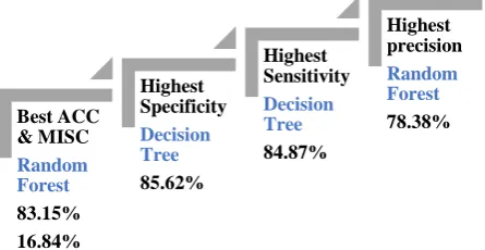
After evaluation each classifier individually, the final step is aimed to compare all of the classification models to determine which model is the most effective in census data. 27 classification experiments were performed. Each experiment was focused on particular points of interest revealing properties or behavior of decision trees, random forests, and the neural networks in particular conditions. Figure 5 summarizes the highest scores of the performance metrics achieved by each classifier. In terms of accuracy, the RF classifier was effective since it had an accuracy rate of 83.15%. In the same way, this classifier had the lowest misclassification rate among other classifiers. Specificity on the other hands, refers to the classifier's ability to exclude an individual who earns less than 50K correctly (which are negative cases). According the experiments results, DT classifier worked well in predicting the negative examples, and it had the highest specificity score of 85.62%. RFs came next with 85.36%. In contrast, the ANNs classifier had lower specificity score with 85.24%.

Figure 5: The Best Scores of Accuracy, Specificity, Sensitivity, and Precision

Sensitivity, on the other hands, refers to the classifier's ability to identify individuals who make over 50K (the minority class.) correctly which is the true positive rate. DT classifier worked well in predicting the positive classes with approximately 84% of sensitivity, which refers to an individual who makes over 50K. DTs overcome RFs and ANNs models which achieved about 80% of sensitivity.

In terms of precision, a RF classifier achieved the highest score with 78.38% of precision. In contrast, DTs and ANNs achieved about 77% of precision.

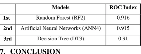
In general, the RF classifier has the best performance for prediction the annual income when compared to other classifiers. It overcomes the ANNs and the DTs classifiers. ROC curve was used for the comparison and to support findings. It aimed to compare the final results for the best models for the decision tree, random forest, and the neural networks. The winners’ models that represent their classifiers are:

72.00% 74.00% 76.00% 78.00% 80.00% 82.00% 84.00% 86.00%

1 2 3 4 5 6 7 8 9

ANN EXPERIMENTS

Accuracy Precision Recal l specificity

Best ACC & MISC

Random Forest

83.15% 16.84%

Highest Specificity

Decision Tree

85.62%

Highest Sensitivity

Decision Tree

84.87%

Highest precision

Random Forest

 Model 1: Decision tree with 3 splits and 5 leaf size (DT3).

 Model 2: Random forest with 50 trees and 7 variables (RF2).

 Model 3: Neural networks with 4 hidden layers (ANN4).

The random forest model achieved the best performance with ROC index of 0.916. The neural networks model came next with a ROC index of 0.915. Therefore, the decision tree model is lowest model with 0.91 ROC index.

Table 11: ROC Index

Models ROC Index

1st Random Forest (RF2) 0.916

2nd Artificial Neural Networks (ANN4) 0.915

3rd Decision Tree (DT3) 0.91

7.

CONCLUSION

This paper aimed to examine and investigate three well-known supervised machine learning classifiers using the United States census data to predict the annual income. It also aimed to determine the most effective classifier to be used in this area. In order to achieve this goal, twenty-seven classification models were created and trained under different settings (parameters). In general, the DT classifier achieved the highest score in sensitivity and specificity. Whereas, the RF classifier achieved the highest score in the accuracy and precision. It is also noted that building a sophisticated model by adding too many features might not improve the prediction accuracy of the model. For example, in the random forest models, selecting 50% of the total number of features achieved the best result. In contrast, selecting 100% of features (all variables) does not lead to rises the performance of RF classification accuracy. It is also noted that the annual income was influenced by some factors. According to the Logworth values generated by decision trees classifier, the variable "relationship" is the most important variable to determine the annual income. In contrast, the variables "native country", "Fnlwgt", "work class", and "race" had the lowest Logworth, and they did not affect the annual income. A RF classifier was considered to be the best classifier since it had the highest ROC index with 0.916. It also had the highest accuracy and the lowest misclassification rate. There are lots of areas that can be carried out in the future. One of the main drawbacks of this study was that the data used in this study was from the 1996 population census which can affect the performance of the classification models. As a result, it is highly recommended to find more recent census data in this study in order to make the models more suitable for today’s populations and for the current census data. Another area of the future work is to investigate different classifiers for predicting the annual income. Several classifiers can be used for this purpose, including Support Vector Machine (SVM), Logistic Regression, Naïve Bayes, and k-nearest neighbors. The future work can also involve the pre-processing step on the dataset because most data can have all kinds of error in it. One of the objectives of conducting census is to collect accurate and complete data from the respondent. But in some cases, respondents may omit required items or provide inaccurate data. So, errors or outliers are more likely to be found in census data. Therefore, the pre-processing steps could be extended to ensures the quality of the data. A number of data pre-processing techniques could be used. Outlier

analysis can be carried out on the dataset, and it is detected by clustering technique.

8.

REFERENCES

[1] Chikohora, T. (2014). A Study of The Factors Considered When Choosing an Appropriate Data Mining Algorithm. International Journal of Soft Computing and Engineering (IJSCE), 4(3), 1-6.

[2] Sumathi, S., & Sivanandam, S. (2006). Introduction to Data Mining and its Applications. Springer-Verlag Berlin Heidelberg. doi:10.1007/978-3-540-34351-6 [3] Hassani, H., Saporta, G., & Silva, E. (2014). DATA

MINING AND OFFICIAL STATISTICS: The Past, the Present and the Future. The journal of big data, 2(1), 34-43. doi:10.1089/big.2013.0038

[4] Wheldon MC, Raftery AE, Clark SJ, Gerland P. Estimating Demographic Parameters with Uncertainty from Fragmentary Data. Center for Statistics and the Social Sciences, University of Washington, Seattle, Washington, 2011, Working Paper 108.

[5] Drummond, C., Matwinm, S., & Gaffield, C. (2000). Inferring and revising theories with confidence: data mining the 1901 Canadian census. Journal of Machine

Learning Research, 1-48.

doi:10.1080/08839510500313711

[6] Nordbotten, S. (1996). Neural network imputation applied to the Norwegian 1990 population census data. Journal of Official Statistics, 12(4), 385-401. [7] Nithya, A., & Sundaram, V. (2011). Wheat disease

identification using Classification Rules. International Journal of Scientific & Engineering Research, 2(9), 01-05.

[8] Malerba, D., Esposito, & Lisi, F. (2002). Mining Spatial Association Rules in Census Data. Intelligent Data Analysis, 541-550.

[9] Han, J., & Kamber, M. (2006). Data Mining: Concepts and Technique (2nd ed.). Morgan Kaufmann.

[10]Witten, I., & Frank, E. (2005). Data Mining: Practical Machine Learning Tools and Techniques (2nd ed.). Morgan Kaufmann.

[11]Breiman, L. (1996). RANDOM FORESTS. Machine Learning journal, 45(1), 1-33.

[12]Ali, J., Khan, R., Ahmad, N., & Maqsood, I. (2012). Random Forests and Decision Trees. International Journal of Computer Science Issues (IJCSI), 9(5), 272-278.

[13]Williams, J., Ahijevych, D. K., Saxen, T., Steiner, M., & Dettling, S. (2008). A machine-learning approach to finding weather regimes and skillful predictor combinations for short-term storm forecasting. American Meteorological Society Journal (AMS), 1-6.

[14]Berry, M., & Linoff, G. (2004). Data Mining Techniques: For Marketing, Sales, and Customer Relationship Management (2nd ed.). Wiley.