R E S E A R C H
Open Access
Backtracking-based dynamic
programming for resolving transmit
ambiguities in WSN localization
Stephan Schlupkothen
*, Bastian Prasse
†and Gerd Ascheid
†Abstract
The complexity of agent localization increases significantly when unique identification of the agents is not possible. Corresponding application cases include multiple-source localization, in which the agents do not have identification sequences at all, and scenarios in which it is infeasible to send sufficiently long identification sequences, e.g., for highly resource-limited agents. The complexity increase is due to the need to solve an additional optimization
pro-blem to resolve the indifferentiability of the agents and thus to enable their localization. In this work, we present a thorough analysis of this problem and propose a maximum a posteriori (MAP)-optimal algorithm based on graph decompositions and expression trees. The proposed algorithm efficiently exploits the fixed-parameter tractability of the underlying graph-theoretical problem and employs dynamic programming and backtracking. We show that the proposed algorithm is able to reduce the run time by up to 88.3% compared with a corresponding MAP-optimal integer linear programming formulation.
Keywords: Wireless sensor networks, Localization, Transmit ambiguities
AMS Subject Classification: 90C35, 90C39
1 Introduction
The unique identification of wireless sensors or agents is generally regarded as an axiomatic design criterion for wireless systems. However, in certain application cases, unique identification is either inherently impossible, such as inmultiple-source localization, or infeasible because of application-specific constraints. In many scenarios, agent localization relies on pairwise inter-sensor distance mea-surements, for which precise information about the iden-tification of the agents and the obtained measurements is required when using classical localization algorithms. In cases in which unique identification is not possible, the localization of wireless agents requires solving an addi-tional optimization problem to overcome the non-unique identification of the agents. In this work, the correspond-ing problem is thoroughly analyzed and an efficient and optimal algorithm is presented. Subsequently, a relevant use case for these algorithms is presented.
*Correspondence:[email protected] †Equal contributors
Integrated Signal Processing Systems, RWTH Aachen University, Templergraben 55, Aachen, Germany
An upcoming application case for wireless sensors in which non-unique identification will play a key role is the exploration of environments that are accessible only by miniature sensors1. Such environments include ground-water systems and, as considered in [1], hardly permeable
cold heavy oil production with sand (CHOPS) mining
areas. In both cases, the idea is to utilize wireless sen-sors to explore the environment and gather information regarding, e.g., the structure of the underground system, the physical properties of the sensor-carrying fluid, and the general resource richness. For these scenarios, the sensor motes need to satisfy the following requirements, which are mainly derived from or mentioned in [1]:
• An outer diameter of less than5mm to ensure that a significant number of the sensors remain intact after passing through the injection pumps.
• A robust shell able to withstand pressures of up to
6MPa [2].
• Several tens of thousands of sensor motes to survey a significant portion of the environment while
accounting for the fact that many sensors will be
destroyed and remain unrecovered in the
environment. In this regard, [1] report an extraction ratio of approximately 8%. The large required number of agents is also motivated by the limited sensing range of each agent.
• Energy supply for an operating time of approximately
48 h.
To facilitate the localization of the agents, they are equipped with ultrasonic transceivers and perform rang-ing by measurrang-ing the round-trip times to other agents. These measurements are only stored locally and are not forwarded to nearby agents. The positioning, i.e., local-ization, of the sensor motes is performed offline after the extraction of the agents by a central unit, which can uti-lize significant computational resources for this purpose. This unit has access to all measurements recorded by the recovered agents.
In this scenario, the following conditions lead to the conclusion that unique identification of the agents is not feasible:
1. The small sensor size and the long operation time significantly constrain the consumable energy, particularly because the majority of the available space inside the agents is already occupied by hardware such as transceivers and environmental sensors.
2. Because of the small sensor mote size and its implications, Direct-Sequence (Spread Spectrum) Code-Division Multiple Access (DS-CDMA) approaches are needed because, e.g.,
frequency-division multiple access (FDMA) and TDMA require both a wide bandwidth and sharp filters2and accurate synchronization, respectively, and thus cannot be used. For DS-CDMA, it is known that the code length is equal to the number of users in the network3. Thus, the use of unique codes would result in excessive power consumption for the transmission of each ranging pulse.
Consequently, only shorter—meaning non-unique—DS-CDMA codes can provide a reduction in the energy requirements that is sufficient to enable this applica-tion scenario4. Therefore, the central unit (fusion center)
needs to resolve the resulting ambiguities in the pairwise distance measurements, before positioning using classical localization algorithms will be possible.
It is believed that a computationally intensive tracking of the agents can be replaced by several quasi-static local-izations whenever the swarm is distributed entirely within the environment. This is because on the one hand many agents are needed for the exploration and because on the other hand it may take long for the agents to pass through the environment. Consequently, a further important task
is to estimate—based on the agent measurements—when these localizations should take place.
Note that the underlying problem of insufficient time or frequency resources to uniquely address all agents can likewise occur in other multiple-access schemes. Addi-tionally, note that there is no negative impact regarding, e.g., the signal processing, hardware resources, or energy consumptions of the agents as a result of the non-unique identification. This is because the increased localization complexity that results from non-unique identification and the resolution of the resulting ambiguities are borne by the fusion center.
In this work, the implications of non-unique identifica-tion for the localizaidentifica-tion of sensor motes are investigated. In this regard, we show that non-unique identification results in an additional optimization problem beyond the actual localization itself. We refer to this additional prob-lem as thetransmit-ambiguity resolution problem(TARP). To address this problem, we propose an algorithm that is able to resolve the ambiguities optimally in the sense of the maximum a posteriori (MAP) probability and that is up to 8.55 times faster than an equivalent integer lin-ear programming (ILP) formulation, which isN P-hard in general and which serves as a baseline in this work. This corresponds to a run-time reduction of 88.5%. The algo-rithms presented in this work are designed to be used in conjunction with classical localization algorithms, such as those based on semidefinite programming [3–9], second-order cone programming (SOCP) [10], or least-squares methods [11, 12], for the described scenarios. Conse-quently, it is said that the presented algorithmsre-enable the localization with existing localization algorithms.
1.1 Related work
Motivated by an initial feasibility study regarding the exploration of inaccessible environments [1] and related experiments in which the need for shared transmis-sion identifiers has been foreseen, the authors of [13] presented the first procedure aimed at resolving the transmit ambiguities caused by non-unique identifica-tion for FDMA-based scenarios. The presented method was heuristic and was not derived from an optimality measure such as minimum mean-squared error (MMSE) or maximum-likelihood (ML). Moreover, its complex-ity was not analyzed, and measurement noise was not explicitly considered. The proposed method relied on a neighbor-matching procedure in which the ambiguities were resolved by comparing the distance measurements of neighboring sensors.
Moreover, in our conference work [16], we introduced the concept of dynamic programming on k-ambiguity trees by exploiting fixed-parameter tractability to effi-ciently solve the TARP. The run time of this method was compared with that of the integer programming imple-mentation of the MMSE-optimal algorithm.
1.2 Contributions
The contribution of this work is fourfold: First, we present a detailed and comprehensive mathematical formulation of the TARP, which arises in the case of the non-unique identification of sensor motes, including the governing equations and its optimal ILP-based optimization prob-lem. Second, we propose to use dynamic programming instead of solving theN P-hard ILP problem to re-enable the localization of the agents. Third, we describe a new representation of the problem using k-ambiguity trees, which are derived fromk-expression trees and are used in a dynamic programming manner to solve the problem optimally. This tree representation is based on a fixed-parameter tractability analysis, which is the basis for the efficient solution of the TARP. Fourth, we improve the dynamic programming approach by employing backtrack-ing, which yields a further reduction in the computational complexity by incrementally evaluating partial solution candidates.
Consequently, we propose a methodology that compen-sates for the inability of these classical methods to address
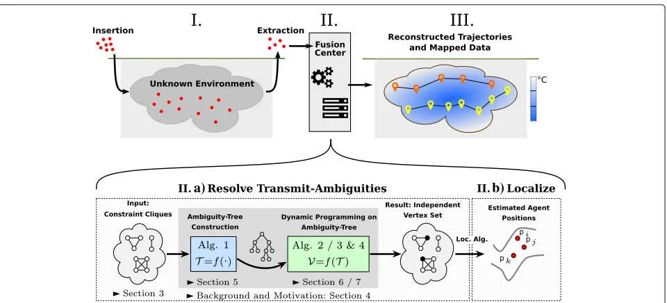
non-relatable distance measurements while maintaining their general applicability for positioning, cf. Fig.1.
This work is partly based on our previous conference work [16], which is extended in this work in terms of the following: (1) detailed derivations of the presented algorithms, (2) an extensive evaluation and analysis of the algorithms, and (3) an algorithmic extension via backtracking, resulting in a new dynamic programming methodology.
Moreover, the framework developed in this work can also be extended, for example, to the multiple-source localization problem, which can be regarded as a special case of the problem at hand in which all sources have the same transmit ID.
1.3 Solution overview
This section is dedicated to a less formal description of the problem at hand and the solution steps described in this work. The sensory-agent-based approach for the explo-ration of unknown environments is depicted in Fig.1. This figure shows the general procedure, from the introduction of the agents up through their (partial) extraction and the utilization of the agents’ measurements for environmental data reconstruction.
The fusion center, which plays a key role in achiev-ing the goal of obtainachiev-ing precise information about the underground environment, must address the non-unique identification of the agents and their consequently
non-a) b)
relatable distance measurements. In this regard, the fusion center follows a two-step approach, where the transmit ambiguities are first resolved and then localization is conducted:
1. The resolution of the transmit ambiguities:
Conceptually, the purpose of this step is to estimate the proper mapping between the measurements and the agents. In this work, however, a mapping between pairs of measurements and pairs of agents is sought. Such a pair of measurements is called anassignment orsolution candidate for the two bidirectional measurements between the corresponding pair of agents. Because of the combinatorial nature of this problem, it isN P-hard in general. As shown in Section3, this problem is related to theindependent set problem and can be described as an ILP problem. However, Section4motivates the use of dynamic programming to solve this problem more efficiently based on the fact that the problem isfixed-parameter tractable. In this context, it is shown that the
clique-width of the graph that describes the resolution problem from a graph-theoretical perspective exerts a significant influence on the solution complexity. For this reason, the following procedure is used in this work to solve the problem:
(a) Based on a thorough analysis of the graph-theoretical problem presented in Section4, the constraints that govern the combinatorial problem are derived. These constraints are described by vertex sets specifying mutual exclusivity, called constraint cliques in the following.
(b) These constraint cliques, which are the basic entities of the graph-theoretical problem, are used to obtain a tree structure that serves as the basis for computing the complexity-determiningclique-width parameter. This computation is performed such that, with a reasonable computational complexity, a complexity parameterk close to the actual clique-width —which is the lowest possible k —is achieved. The corresponding theory and algorithm are introduced in Sections4and5. (c) Utilizing the previously computed tree
structure, dynamic programming methods are used to obtain a solution. The solutions correspond toselected vertices of the vertex sets that specify the mutual exclusivity of the constraint cliques. Consequently, a solution to the combinatorial problem is found, and a mapping between the measurements and the agents is obtained. Two different dynamic
programming algorithms are presented in Sections6and7, of which the latter uses a backtracking procedure.
2. The localization of the agents: Based on the mapping between the measurements and the agents, classical localization algorithms can be used for positioning. See, e.g., the last paragraph of Section1for an overview of possible solution methods.
1.4 Organization
Based on the steps outlined in Fig. 1, the remainder of this work is structured as follows. In Section 2, the system model and problem formulation are presented. Section3introduces the constraints that govern the class of input problems and their graph-theoretical description (Fig. 1, II.a first step). This special graph structure will be exploited in the proposed algorithm to efficiently solve the TARP. Finally, this section presents an overview of the ILP-based problem formulation. Section 4 summarizes the theoretical foundations of the proposed algorithms and introduces the concepts of, e.g., fixed-parameter tractability and expression trees, which are needed for the subsequent discussion of the algorithm design. The pro-posed algorithms consist of two steps, which are described in Section5(Fig.1, II.a second step) and Section6(Fig.1, II.a third step). Section5shows how the graph-theoretical problem can be described using a special variant of the clique-width k-expression tree. In Section6, this expres-sion tree is used in a dynamic programming algorithm to resolve the transmit ambiguities. An improved back-tracking version of this dynamic programming algorithm is described in Section7(Fig.1, II.a third step). A numer-ical evaluation of the presented methods is presented in Section8, and Section9gives a summary and an outlook regarding future work. To illustrate how the presented algorithms operate, Appendix 1provides corresponding examples.
2 Problem introduction and system model
and fixed. The following steps are performed to enable the localization of the sensor motes:
1. The agents, equipped with ultrasonic transducers, are introduced into the environment.
2. The agents record measurements of physical properties such as pressure and temperature. In addition, the agents perform round-trip time (RTT) measurements to facilitate distance estimates to neighboring agents. Because of the strict energy limitations, there is no forwarding or transmission of any data aside from the RTT measurements.
3. The agents are recovered from the environment, and their RTT measurements are jointly processed by the transmit-ambiguity solver to overcome the
ambiguities in the distance measurements.
4. Classical localization algorithms are used to estimate the positions of the agents for each time instance when an RTT measurement was made.
The inaccuracy of the RTT ranging procedure is mod-eled as multiplicative noise. In this model, which has also been adopted by, for example, [7], it is assumed that dis-tance estimates to farther sensors are less accurate. Conse-quently, the random variable (RV)dj→i, which denotes the distance measured by sensoribased on a ranging pulse sent by sensorj, is given by
dj→i=di,j
1+ni,j
(1)
where allni,j ∼ N
0,σi2,jare independently and
identi-cally distributed (iid) Gaussian variables with varianceσi2,j. Moreover, it is assumed that bidirectional measurements are made. Note that bidirectional communication is also a requirement for RTT measurements. Hence, it is assumed that if sensorimeasured a distance to sensorj, then sensor jalso measured a similar distance with respect to sensori. An illustration of the notation is given in Fig.2. The set of RVs referring to the range measurements received by sensor motei, which uses IDIL, from nodes sending with
IDIK is denoted byDi = {dj→i|j ∈ K}. The set of dis-tances that sensorihas measured with respect to sensors usingIK is denoted by Mi =
m1i,m2i,. . ., where mli denotes the correspondinglth range measurement of sen-sor i5. As full connectivity is not necessarily given, the following holds: |Mi| ≤ |Di|. Consequently, Mi is an unordered or permuted subset of the random variates, i.e., realizations, of the RVsDi.
The following definition of the derived problem is used.
Definition 1 (transmit-ambiguity resolution problem (TARP)) The TARP is the problem of overcoming the inability to differentiate among agents that use the same transmit code during communication. In the context of RTT ranging, e.g., for the sake of agent localization, the TARP is the problem of finding the correct mapping
between the distance or RTT measurements mli and the
RVs dj→iand, thus, the agents. Thereby, a decision is made regarding the source of a ranging pulse and its resulting distance or RTT measurement.
An important aspect of the algorithm derivation and the henceforth used notation is that the TARP can be decom-posed into independent subproblems, which are given by all pairs of—not necessarily distinct—IDs. In this regard, notice that the ambiguities occurring between two (dis-tinct) groups of agents, each with possibly individual IDs, are not affected by measurements or ambiguities with any other groups of agents. This fact is also illustrated in Fig.3a. Because of the independence of the subproblems and without loss of generality, only the measurements between sensor motes using, as an example, the IDsIK andILare considered in the following.
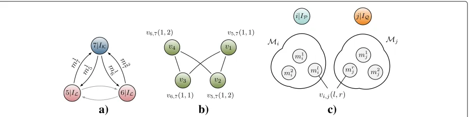
Example 1An example of the consequences of the reuse of DS-CDMA codes with respect to localization is illus-trated in Fig. 3a. This figure shows two sensor motes, “5” and “6,” that are both using ID IL. A third sensor mote (“7”) is using ID IK. Because the sensor motes can
a)
b)
c)
Fig. 3 aIllustration of a network with non-unique identification sequencesIKandILand their respective distance measurements as seen by the receiving node [14]. The gray arrows and their corresponding measurements are not considered in the subproblem betweenIKandIL.
bAmbiguity corresponding toa, wherev5is given by the pair of measurements indicated in gray between agents “5” and “6.” For clarity, the edges are annotated with the measurements that give rise to them (cf. items 1(a) and 1(b) in the listing in Section3). Independent of the previous example, cprovides a general illustration of how verticesvi,j(l,r)are formed based on the measurement setsMiandMjof agentsiandj, respectively
differentiate only between different DS-CDMA codes and not between different sensor motes that are using the same code, sensor mote “7” measures two distances that can-not be related to sensor motes “5” and “6.” More precisely, sensor mote “7” measuresM7 = m17m27 (realizations
of the RVs contained in D7 = {d5→7d6→7}), and before
offline localization can be performed, the mapping between these measurements and sensors “5” and “6” needs to be estimated.
Consequently,classicallocalization methods, which do not consider application scenarios with transmit ambi-guities—such as [3, 6, 7], which use semidefinite pro-gramming, or [11], which uses a linearized least-squares approach—cannot be used without first applying algo-rithms to resolve the TARP such as those presented in this work.
3 Graph representation and graph problem
formulation
In this section, a graph-theoretical formulation of the problem resulting from DS-CDMA code reuse is given. Moreover, a detailed analysis of the problem’s properties, which will be exploited in Section4, is presented.
The following description utilizes the particular prop-erties of a type of graph whose instances are henceforth calledambiguity graphs. Such a graph is denoted byG = (V,E,W), and its components, i.e., the vertex set, edge set and weight function, are defined in the following.
Every vertex of the ambiguity graph is uniquely identi-fied by the notationvi,j(l,r), whereiandjrefer to agents
i andj andl and rrefer to their respective lth and rth measurements. Therefore, the vertexvi,j(l,r)refers to the
RVs(dj→i,di→j) and their potential realization given by the measurements
mli,mrj
. In the following, this relation
is denoted byvi,j(l,r) ref.∼
mli,mrj
. Moreover, this vertex has a weight, which corresponds to the likelihood that the
measurements mli andmrj were both measured between agentsi andj. This section describes how this weight is calculated and presents the definition of the edges of this graph.
Example 2A simple example of an ambiguity graph for a network is shown in Fig.3a. For simplicity, a linear index vkis used to denote the vertices of the ambiguity graph. The relationship between this linear notation and the vi,j(l,r)
notation is as follows: v1 = v5,7(1, 1), which relates to
m15,m17; v2 = v5,7(1, 2), which relates to
m15,m27; v3 =
v6,7(1, 1), which relates to
m17,m16; and v4 = v6,7(1, 2),
which relates to m16,m27. With this short-hand nota-tion, the edge and vertex sets for this example are given as follows:E1,a(5, 1) = {(v1,v2)}, E1,a(6, 1) = {(v3,v4)},
E1,b(7, 1) = {(v1,v3)},E1,b(7, 2) = {(v2,v4)},E2(5, 7) = {(v1,v2)}, E2(6, 7) = {(v3,v4)}, V1,a(5, 1) = {v1,v2},
V1,a(6, 1) = {v2,v4}, V1,b(7, 1) = {v1,v3}, V1,b(7, 2) = {v2,v4},V2(5, 7)= {v1,v2}, andV2(6, 7)= {v3,v4}.
The set of edgesEof the ambiguity graph is the union of three edge sets that satisfy the criteria given below.
1. In the following problem descriptions, edges are used to denote complementary constraints, and any distance measurementmlican be assigned to only one RVd•→i; therefore, edges are introduced as follows:
(a) Betweenvi,j(l,r)ref.∼
mli,mrj
and any other
vertexvi,j(l,r)
ref.
∼ mli,mrj
that relates tomli. The set of all edges created based on this condition is denoted byE1,a(i,l).
E1,a(i,l)=
(vx,vy)∈V×V vx
ref.
∼ mli,mrj∧vy
ref.
∼mli,mrj
(b) Betweenvi,j(l,r) The set of all edges created based on this condition is denoted byE1,b(j,r).
be matched to at most one tuple of measurements, i.e., one vertex of the ambiguity graph. Therefore, edges are introduced between any vertexvi,j(l,r)and
vi,j(l,r), i.e., any other vertex that corresponds to the same bidirectional link between sensorsi and j. The set of all edges created based on this condition is denoted byE2(i,j).
to the corresponding (sub)item and its constraints as given in the listing above.
The objective is to maximize the probability P of correctly matching the RVs to the distance measure-ments given all measuremeasure-ments Mi from all sensors i, i.e., the noisy distance measurements. A derivation of the PDF
used in the numerical evaluation of this work is given in Appendix2.
Thus, the construction of the ambiguity graph G = (V,E,W)can be summarized as follows: possible solution candidate for the measurement assignment problem. More precisely, it reflects the probability thatmliandmrj are the realizations ofdi→j
anddj→i, respectively. In the subsequently described
optimization problem, the goal will therefore be to select a subset of these solution candidates.
• The likelihood that the mapping denoted byvi,j(l,r) is correct is given by the corresponding weight
W(vi,j(l,r)).
• The edges (cf. Eq. (5)) govern the criteria under which a solution candidatevi,j(l,r)may be selected. Note that the vertices that are subject to particular constraints, such asE1,a(i,l),E1,b(j,r), orE2(i,j), are the vertices that are the endpoints of the edges in these sets. The corresponding sets of vertices and their subgraphs are denoted byV1,a(i,l),V1,b(j,r), because by the definition of item 1(a) in the listing above,vi,j(l,r)is adjacent to any other vertex that relates to the measurementmli, and by the definition of item 1(b),vi,j(l,r)is also adjacent to any other vertex that relates to the measurementmrj. Moreover,
vi,j(l,r)is a solution candidate for the measurements between agentsi and j and hence is also an endpoint of the edges inE2(i,j)and is therefore adjacent to the vertices inV2(i,j).
For brevity and simplicity, in the following, we may refer to the verticesvi,j(l,r)asvk,k ∈ {1,. . .,|V|}, if the addi-tional information provided by the indicesi,j,l, androf vi,j(l,r)is not relevant.
where xk is either one or zero and indicates whether vertex k of the ambiguity graph is in the solution set or not, respectively. This means that any measurements
mli,mrj that are in the solution set, i.e., whose cor-responding vertices vi,j(l,r) are in the independent set,
are chosen as the realizations of the RVs (dj→i,di→j). Furthermore, wk denotes the weight of vertex vk ∈ V, i.e., wk = W(vk). Constraint (8e) ensures the inde-pendence of the set by allowing at most one of two adjacent vertices to be included in the solution set. Con-straints (8b) to (8d) refer to the conditions described in items 1(a), 1(b), and 2 of the listing above and consti-tute additional constraints compared with the classical independent set problem; they are calledsize constraints because they enforce independent sets of a particular size.
Note that because of the choice of the vertex weights (cf. Eq. (7)), the solution to Problem (8) corresponds to the feasible solution with the highest probability in the MAP sense (cf. Eq. (6)). In addition, note that Problem (8) is N P-hard in general [17,18].
4 Exploiting the graph structure
Because of the N P-hardness of Problem (8), new algo-rithms are needed that can solve the TARP optimally but more efficiently than regular ILP solvers. Less compu-tationally complex algorithms are particularly necessary to accommodate the large number of agents needed for the considered application case. The idea that serves as the basis for the following sections is to employ dynamic programming to obtain a highly tailored algorithm to facilitate efficient solution generation. This is enabled by exploiting the special graph structure described in Section 3. The underlying principle of this exploita-tion is the fixed-parameter tractability (FPT) of the problem.
In this regard, Section4.1introduces the concept of FPT and a theorem that renders it applicable to the TARP and thereby forms the basis of our chosen dynamic program-ming approach. Section 4.2presents an overview of the fundamental graph-theoretical concepts, including graph decomposition, that enable the application of the FPT theorem to the TARP. Based on these concepts, Section5 introduces a novel variant of this decomposition that is tailored to ambiguity graphs.
4.1 Fixed-parameter tractability
The concept of FPT is generally used to analyze problems and, in particular, to find which parameters significantly influence the computational complexity. This analysis can then be used to design efficient algorithms for solving N P-hard problems such as the TARP.
The idea of FPT is to describe the complexity of anN P -hard problem as a combination of two aspects: the first depending only on the input, such as the number of ver-tices of a graph, and the second being given by somefixed parameterof the problem. Generally, a problem is said to be fixed-parameter tractable if some algorithm capable of solving this problem has a complexity ofO(poly(|x|)f(k)), where |x| denotes the size of the input, poly(·) denotes some polynomial function, and f(k) is some arbitrary function of the fixed parameterk[19].
The algorithm proposed in this work is based on a theorem presented by [20], which states that finding the independence number, i.e., the size of the largest indepen-dent set, is a fixed-parameter tractable problem in which the complexity parameterkrefers to a graph property or parameter known as theclique-width. Theclique-widthis introduced in detail in Section4.2below. Regarding the applicability of this theorem to the TARP, note that in Problem (8), the goal is to find an independent set with a particular independence number that is given by the num-ber of distinct sets of typesE1,a(·,·)andE1,b(·,·)6. Because
the decisionvariant of finding the independence number can be interpreted as answering the question “is there an independent set with a size of at leastn?”, the following theorem is applicable to Eq. (8).
Theorem 1(The problem of finding the independence number is fixed-parameter tractable [20])The problem of
determining the independence number of a graph G =
(V,E)with a clique-width of at most k has a complexity of O(|V|f(k))ifGis given by a clique-width k-expression.
Consequently, Theorem1states that the clique-widthk of graphGis an important parameter when the desire is to find the independence number ofG. This is highlighted by the fact that for the problem of finding the independence number, [21] specifies the particular functionf(k) = 2k to concretize the complexity in the FPT theorem above [22]. Consequently, the objective in the following is to find a clique-widthk-expression for instances of the ambi-guity graph with the minimum possible clique-width k. However, computing the clique-widthk of a graph is an N P-hard problem in general [23]. Therefore, sub-optimal methods for finding some approximation k ≥ k of the clique-width are presented in this work.
modeled using a tree. In this way, a graph is said to be decomposed, e.g., into a tree structure.
Remark 1The motivation for using tree-structure decompositions of graphs, such as tree-decompositions or clique-width k-expression trees, stems mainly from the fact that the independent set problem, for example, can be efficiently solved by applying dynamic programming on such a representation (tree structure)[20, 24]. Our par-ticular interest in decomposing graphs into clique-width k-expression trees is mainly driven by the FPT theorem introduced above and by the fact that the clique-width is upper bounded by the tree-width[25]. Furthermore, note that in our case, in which the decomposition of ambigu-ity graph instances is desired, the edge setE is given by a union of cliques7(cf. Eq.(5)), which turns out to simplify the formulation of an expression for the clique-width.
4.2 Graph theory definitions and notations: clique-width
Recall that, motivated by Theorem1, the goal is to find clique-widthk-expressions that correspond to ambiguity graph instances to enable efficient algorithms for solving the TARP. To this end, this section reviews the definitions of the clique-width and clique-widthk-expression trees; this discussion is mainly based on [20,21].
The clique-width is calculated based on recursive oper-ations on vertex-labeled graphs [20]. These operations construct a new clique-width k-expression tree. In the following,G = (VG,EG,labG)denotes ak-labeled graph where each vertex label is given by the mappinglabG : VG →[k], with [k] being the set of natural numbers [k] :=
{1,. . .,k}[21].
Definition 2(Clique-width [20,21])The clique-width of a graphG = (V,E)is the minimum number of vertex labels lab:V →[k]such thatGcan be constructed by the following operations:
• Disjoint union of vertex-labeled graphs: Let
G=(VG,EG,labG)∈CWkand
J =(VJ,EJ,labJ)∈CWkbe two vertex-disjoint
labeled graphs; then,G⊕J :=(V,E,lab)is also in
CWk, withV:=VG∪VJ,E:=EG∪EJ, and
lab(u):=
labG(u) ifu∈VG labJ(u) ifu∈VJ
• Edge introductionsηi,j:ηi,j(G):=(VG,EG,labG),
where
E
G :=EG∪u,v u,v∈VG,u=v, labG(u)=i,labG(v)=j
• Vertex relabelingρi→j:ρi→j
G:=(VG,EG,labG), where
labG(u):=
labG(u) iflabG(u)=i
j iflabG(u)=i ,∀u∈VG
The resulting expression is called a clique-width k-expression or a CWk-expression.
Using Definition 2, a CWk-tree can also be defined, where the root of the tree corresponds to the original unlabeled ambiguity graphG. Consequently, at the rootr of the expression tree, which corresponds to the complete expression, all vertices must have the same label such that the root of the tree is equal to the unlabeled graphG.
Table1presents examples ofCW2-expressions and the
corresponding graphs. Note that onlyk = 2 labels are required to representG6, which has four vertices.
Example 3Figure4shows the CW2-tree for the labeled
graphG6given in Table1. The vertices of the tree are
anno-tated with the induced subgraphs of the tree nodes8. Note that in this example, the original graph,G6, was already
labeled, and hence, the root of the CWk-tree is identical to the original graph, with the same labels.
Generally, the decompositions into CWk-expressions and CWk-trees are not unique, i.e., multiple possible CWk-trees exist for a given graph. The main benefit of representing a graph according to Definition2is that the CWk-expression is directly related to the complexity of the MW-ISP-SC, which is ofO(|V|2k).
Moreover, the attempt to solve such a problem using the CWk-treeT is motivated by the property that the vertex set of subgraphGs, which corresponds to tree nodes, is partitioned intok ≤ |Vs|sets, as given by theklabels [20]. The reason for this is that during the decomposition of a graph into aCWk-expression tree, the labeling will be performed such that, in the dynamic programming phase,
Table 1CW2-expressions and their corresponding 2-labeled
graphs [20]
Graph CW2-expression
G1 1 •1
G2 2 •2
G3 1 2 G1⊕G2
G4 η1,2(G3)
G5 ρ2→1(G4)
Fig. 4CW2-expressions and their corresponding 2-labeled graphs [20]
it is sufficient to differentiate between groups of vertices that have different labels.
Example 4Considering the independent set problem as an example, the independence criterion does not need to be checked for every vertex because all vertices that have the same properties in this regard will have the same label. This is ensured by the design of the labeling function, which is described in the following section. Consequently, for a group of vertices with the same label, a check for independence requires only a single check rather than one check for each vertex in that group.
5 Thek-ambiguity tree
To enable the exploitation of the property mentioned in the FPT theorem, i.e., that the clique-width of the input graph is a critical parameter in determining the com-plexity of the TARP, an algorithm for obtaining the tree description—often called a graph decomposition in the literature, as it disassembles parts of the graph into a tree structure—and related operations are presented in this section. To this end, Section5.1introduces a short-hand, tailored version of the operations used in theCWk -expressions. The main difference compared with theCWk operations is from a special design criterion that is sub-sequently introduced, which leads to the introduction of additional predefined edges. The tree corresponding to this tailored description is called the k-ambiguity tree in the following. Contrary to the notation of the CWk -tree, the leaves of the k-ambiguity tree are chosen to
be the subgraphs that correspond to the edge constraint sets E1,a(·,·), E1,b(·,·), and E2(·,·), cf. Eqs. (5a), (5b),
and (5c). These subgraphs are denoted by G1,a(·,·) =
V1,a(·,·),E1,a(·,·)
, G1,b(·,·) =
V1,b(·,·),E1,b(·,·)
, and G2(·,·)=(V2(·,·),E2(·,·)), respectively. Note that
accord-ing to the definition of the edge constraint sets, they are complete induced9subgraphs, i.e., cliques10.
Recall, from the definition ofCWk-expressions, that any expression with the operators⊕,ηi,j, orρi→j, e.g., in the form of X1 ⊕X2, in the CWk-tree corresponds to the mergingof two treesTX1andTX2that, in turn, correspond to the expressionsX1andX2, respectively. Consequently,
we use μ(T1,T2) to denote a joint operator that applies
a sequence of ⊕, ηi,j, or ρi→j operations to serve as a mergingoperator. This joint operator is motivated by the canonical form of the clique-width expression [26], in which after each disjoint union⊕, first, several edge intro-ductionsηi,j and then several relabeling operationsρi→j must occur [20].
During this merging process, the key idea is to choose an operation such that its output is aninducedsubgraph ofG. This is because the number of labels required for induced subgraphs is lower than that for non-induced subgraphs11. Thismergingoperation is described in more detail below.
5.1 The merging operator
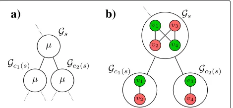
The merging operator performs the steps listed below, thereby merging the labeled subgraphsGc1(s)andGc2(s)to yield the outputGs = (Vs,Es,labs). In the following, we use the indexci(s),i = 1, 2, to represent the edge or vertex set of the first or second child of tree nodes(see also Fig.6a).
1. Union of the children’s vertex sets:
Vs = Vc1(s)∪Vc2(s).
2. Union of the children’s edge sets and a further edge setEc1(s),c2(s):Es = Ec1(s)∪Ec2(s)∪Ec1(s),c2(s). The additional edge setEc1(s),c2(s)is chosen such thatGsis an induced subgraph, which—as mentioned
above—is the desired criterion for the merging operator. Note thatGc1(s)andGc2(s)are both also induced subgraphs, as they are also the results of merging or are cliques corresponding to leaves of the tree. Therefore, the setEc1(s),c2(s)contains only edges of the form(vi,vj),vi∈Vc1(s),vj∈Vc2(s).
3. Vertex relabeling resulting in the fewest possible labels,minlabs|
labs(v)|v∈Vs
|.
The labeling function required to perform steps 2 and 3 is defined in the following. Recall from Section3 that every vertexvi,j(l,r)is an element of exactly three cliques,
namely, G1,a(i,l), G1,b(j,r), and G2(i,j). Because of this
property, all vertices that are adjacent tovi,j(l,r)are in the
Because the k-ambiguity tree corresponding to the ambiguity graph needs to reflect an increasing number of the properties of the original graph as the considered tree node becomes closer to the root of the tree, and in particular because the root of the tree represents the original graph, a tool is needed for describing which prop-erties of a vertex of the original graph are not currently considered at a given tree node. To this end, a func-tionRs(vi,j(l,r))is defined that describes the properties
of a vertexvi,j(l,r)with respect to its originally adjacent
vertices. More precisely,Rs(vi,j(l,r))indicates the
mem-bership of the three cliques corresponding tovi,j(l,r)with
respect to the subgraphGsat tree nodesand is defined as follows:
Rs(vi,j(l,r))=
(i,l)·1Vs(V1,a(i,l)),
(j,r)·1Vs(V1,b(j,r)), (i,j)·1Vs(V2(i,j))
(9)
where1Vs(V)is related to the inverted indicator function and is defined as1Vs(V) = 0 ifV ⊆ Vsand 1 otherwise. Thus, a missing edge to a vertex to whichvi,j(l,r)was
orig-inally connected is indicated by a non-zero tuple entry. An illustration of this function is provided in Fig.5.
Considering the labeling of the vertices, every occurring three-tuple value ofRsis chosen to correspond to a dis-tinct label in the subgraph of tree nodes. Thus, the tuple elements of two vertices,Rc1(s)(v1)andRc2(s)(v2), are suf-ficient to determine whether an edge must be inserted betweenv1andv2by the operatorμ(orηi,j): iff the val-ues and positions of at least one tuple entry in each of Rc1(s)(v1)andRc2(s)(v2) are equal and non-zero, then an edge is inserted betweenv1andv2. This is because these
vertices are part of the same clique in the ambiguity graph,
cf. Section3. Recall that a tuple entry of zero indicates that all edges for the corresponding clique have already been inserted.
Moreover, the function Rs determines the relabeling according to the operatorμ(orρi→j). IffRs(v1)=Rs(v2),
i.e., if the complete tuples are equal, thenv1 andv2 are
assigned the same label ats, as illustrated in the following example.
Example 5We consider two vertices v1 and v2 at tree
node s and assume that Rs(v1) = (0, 0),(1, 1),(0, 0) =
Rs(v2). Then, v1and v2are both lacking edges to all
ver-tices in clique V1,b(1, 1) that are not in Vs, i.e., to all v∈V1,b(1, 1)\Vs. Consider the merging of tree node s with another tree node s by operatorμ: if an edge is inserted between v1and v3∈Vs, then an edge must also be inserted between v2and v3because v1and v2have the same
prop-erties with respect to their current clique memberships. Therefore, no distinction is needed between vertices v1and
v2with respect to the edge insertion operation, and
con-sequently, the same label is assigned to both vertices. This label is uniquely determined by Rs(v1) = Rs(v2).
Note that no two vertices are part of the same three cliques (cf. Section3), and hence, two vertices can have the same label only if at least one tuple entry ofRsis zero for both vertices. At the rootrof the ambiguity tree, which corresponds to the entire ambiguity graphG, all edges are already inserted andRr(vi) = ((0, 0), (0, 0), (0, 0))∀vi ∈
V; therefore, only a single label is needed.
5.2 Building thek-ambiguity tree
Using the methods and, in particular, the merging operator defined previously, this section introduces an
Fig. 5Illustration of a tree nodesand its vertex setVs, which is used to visualizeRs(v)for the two verticesvi,j(l,r)andvi,j(l,r). The corresponding
vertex sets forvi,j(l,r)areV1,a(i,l),V1,b(j,r), andV2(i,j)and are indicated by dashed contours. The setsV1,a(i,l),V1,b(j,r), andV2(i,j)forvi,j(l,r)
are shown with dotted contours. The setV1,b(j,r), which is considered for both vertices, therefore has a dash-dotted contour. The purpose of
visualizingRs(v)for the two vertices is to check whether all vertices of the abovementioned setsV•(•,•)are already included in the vertex setVsat
the current tree nodes. For the two vertices in the example above, we haveRs(vi,j(l,r))= (0, 0),(j,r),(0, 0)=Rs(vi,j(l,r))because for both
algorithm that is able to generatek-ambiguity trees based solely on the subgraphsG1,a(·,·),G1,b(·,·), andG2(·,·).
Because finding the clique-width decomposition of a graphGis anN P-hard problem in general, the decompo-sition of an ambiguity graph into ak-ambiguity tree can also be efficiently done only in a sub-optimal way. Con-sequently, only decompositions that require a number of labels greater than the clique-width are of computational interest. However, note that for such a decomposition, there is no need to build the actual ambiguity graph because the equivalent information is also provided by all subgraphs of typesG1,a(·,·),G1,b(·,·), andG2(·,·). A subset
of these basic entities is therefore chosen as the leaves of thek-ambiguity tree. Note that choosing these cliques as the leaves results in an entry of zero inRs(v)for each ver-texv∈ Vs. The purpose of this heuristic is to reduce the number of distinct three-tuples at tree nodes closer to the root of the tree and thereby reduce the number of labels.
To simplify the notation in the following steps, C is used to denote the set that contains all cliques of types G1,a(·,·),G1,b(·,·), andG2(·,·). Similarly, alllabeledcliques
The setT is the set of all partial ambiguity trees, i.e., all possible branches of the ambiguity tree that relate to a certain subgraph of the ambiguity graph G. Further-more, the neighborhoodN(Gi)of a labeled subgraphGi= (Vi,Ei,labi)consists of those subgraphsGj= (Vj,Ej,labj) that have a corresponding element inT and are adjacent to each other in the ambiguity graphG=(VG,EG):
Gj∈N(Gi)⇔ ∃(vi,vj)∈Vi×Vj such that (vi,vj)∈EG
(10)
Note that when two subgraphsGiandGjare merged that are not in each other’s neighborhoods, the merging out-comeμ(Gi,Gj)requireslabi+labjlabels. In the opposite case, fewer labels may be required.
The greedyk-ambiguity tree construction algorithm is presented in Algorithm 1. On Line 7, it makes use of the remainder graph(V,E,lab)= (G,T), which has the following properties:
• It is the labeled induced subgraph with vertices
V=VG\Vin, whereVin⊂VGis the subset of vertices that already occur in subgraphs corresponding to elements ofT.
• Because it is an induced subgraph, its edge set is given by the edges in ambiguity graphGwhose endpoints are both in the vertex setV[27].
• Moreover,(G,T)is a complete graph, and hence, its edge set can be easily determined.
6 Solving the TARP on thek-ambiguity tree
As shown in Fig. 1, the TARP is solved in two steps, of which the first—i.e., the computation of thek-ambiguity tree—has been presented in the previous section. The second step, in which dynamic programming algorithms are used on the k-ambiguity tree to solve the TARP, is presented in this section.
As mentioned in Section3, the optimal solution to the TARP corresponds to the solution to the MW-ISP-SC with respect to the ambiguity graph. To solve this prob-lem using dynamic programming on the ambiguity tree, an algorithm similar to the method presented by [20] for determining the independence number of a graph is used. However, two major extensions are made to obtain an algorithm suitable for solving the TARP:
1. Accounting for the weight of an independent set in addition to its size
2. Ensuring feasibility with respect to constraints (8b) to (8d)
In the following, additional notations and concepts are introduced that are needed to describe the dynamic pro-gramming algorithm.
The power set of all labels available at a tree nodesis denoted byP([κ(s)])and lists all 2κ(s)possible combina-tions of labels, including the empty set, e.g.,
P([κ(s)])= {∅,{1},. . .,{κ(s)},{1, 2},. . .,{1,. . .,κ(s)}} (11)
Moreover,Ls(V) = {labs(v)|v ∈ V}denotes the set of labels of all vertices inV⊆Vs.
The algorithm proposed hereafter utilizes the following tuple structure. At each tree nodes, which corresponds to the subgraphGs = (Vs,Es,labs), we define
The corresponding most generic optimization problem for computing the data structure F(s) is given in the following. Note that for consistency with the following sections, the elements ofF(s)are denoted bydL. The data structures of the children of tree nodesare denoted by F(c1(s))=(. . .,aL,. . .)andF(c2(s))=(. . .,bL,. . .), cf.
Fig.6a. The elements are given by
Algorithm 1:Greedyk-ambiguity tree construction Input: Clique membership information, i.e.,Clab Output:max-ambiguity treeT
1 T ← ∅; /* initialize partial tree set */
2 S(n)←Gs=(VGs,EGs,labGs)∈Clab |VGs| =n
,∀n∈N; /* given subgraphs that can be labeled
with n labels */
3 max←minGs∈Clab|VGs|; /* upper bound on number of labels */
4 repeat
5 foreachGs∈S(max)do /* update S(max) */
6 If there is no vertex inVGsthat is part of a subgraph whose tree is inT, add the ambiguity tree
corresponding toGs—which is a single leaf—toT. RemoveGsfromS(max)and continue the loop; 7 If some but not all vertices ofVGsare part of a subgraph corresponding to a tree inT, add the remainder
graph(Gs,T)toS(max). RemoveGsfromS(max)and continue the loop;
8 If all vertices inVGsare part of a subgraph corresponding to a tree inT, removeGfromS(max)and
continue the loop;
9 end
10 foreach(TGi,TGj)∈T ×T whereGi∈N(Gj)do /* merge neighboring graphs */
11 Gmerge←μ(Gi,Gj);
12 IfGmergehas at mostmaxlabels, removeTGiandTGj fromT. Add the treeTGmergecorresponding toGmerge toT;
13 end
14 If Line 12 has never been executed, i.e., no trees fromT have been merged, increase the label boundmaxby one;
15 untilT contains only one element, which represents the complete ambiguity graphG;
where the weightsW(vi)are given by Eq. (7). To enable the recursive computation ofF(s),dL is obtained as
dL = min
V1,V2
vi∈V1∪V2
W(vi) (14a)
s.t. Ls(V1∪V2)=L (14b)
V1⊆Vc1(s),V2⊆Vc2(s) (14c)
because the vertex set corresponding to tree nodes,Vs, is the union of the vertex sets of the children ofs. By the
def-a)
b)
Fig. 6Examples ofk-ambiguity trees.ashows a part of a tree in which the tree nodes consist of the merging operatorμ. This visualization is analogous to the general description of clique-widthk-expression trees, in which the annotated ambiguity subgraphsGare often referred to asbags.bshows the same tree, with the tree nodes—for clarity—replaced by the corresponding labeled ambiguity subgraphs
inition of theCWk-tree (cf. Definition2), for the objective function of Problem (14), it holds that
min
V1,V2
vi∈V1∪V2
W(vi)= min
V1,V2
vi∈V1
W(vi)+
vi∈V2
W(vi)
(15)
and for the first constraint of Problem (14), it holds that
Ls(V1∪V2)=Rc1(s)→s
Lc1(s)(V1)
=:L1
∪Rc2(s)→s
Lc2(s)(V2)
=:L2
(16)
whereRci(s)→s
Ldenotes the label set at tree nodesof the vertices labeled withL atci(s).
Algorithm 2:TARP-Solver based on dynamic programming on ak-ambiguity tree Input:k-ambiguity treeTof ambiguity graphG
Output: Vertex set corresponding to the optimal solution to Problem (8)
1 Start bottom-up dynamic programming;
2 repeat
3 Determine the subgraphGs=(Vs,Es,labs)corresponding to tree nodes;
4 ifs is a leaf of Tthen
5 ComputeF(s)=a∅,a{1},. . .,a{1,...,κ(s)}as follows:
6 ifGsis of typeG1,aorG1,b, i.e.,Gs∈C1,abthen
7 aL = v∈Vs(L)W(v) if|L| =1
∞ else
8 else /* Gs is of type G2 */
9 aL = v∈Vs(L)
W(v) if|L| =1
0 if|L| =0
∞ else
10 end
11 else /* s has two children, c1(s) and c2(s) */
12 AsF(c1(s))=
a∅,a{1},. . .,a{1,...,κ(c1(s))}
andF(c2(s))=
b∅,b{1},. . .,b{1,...,κ(c2(s))}
are known from previous iterations, compute alldL ofF(s)=d∅,d{1},. . .,d{1,...,κ(s)}
according to Problem (17).
13 end
14 untilroot r of T reached;
15 Based onF(r)=(a{1})at the rootrof the tree, recursively obtain the label setsL1andL2that minimize the
objective function of Problem (17). At the leaves, the mapping between the labels and vertices is unique.
6.1 Ensuring the independent set size in thek-ambiguity tree
Constraints (8b) and (8c), which determine the size of the independent set, are equivalent to the requirement that each clique inC1,ab must have exactly one vertex in the solution to the independent set problem. The clique setC1,abis defined as a subset of the clique setC, which was introduced in Section5.2:C1,abconsists of all cliques (complete subgraphs) that are due to ambiguity graph constraints 1(a) and 1(b), i.e., of theG1,a(·,·)andG1,b(·,·)
types. To enable a feasibility check of the size constraint at each tree nodes, letC1,ab(s) ⊆C1,abdenote those cliques whose vertices are completely included in Vs. Now, set aL = ∞if there is no vertex setVwithLs(V)=L that contains a vertex fromeveryclique inC1,ab(s).
Example 7 If, e.g., Rc1(s)(v) =
(α1,α2),(β1,β2), (γ1,γ2) with α1,α2 > 0 (cf. Eq. (9)) and Rs(v) =
(0, 0),(β1,β2),(γ1,γ2)
, then G1,a(α1,α2) is in C1,ab(s),
and hence, at tree node s, exactly one vertex v ∈
V1,a(α1,α2)must be selected as part of the independent set
solution. Therefore, it is said that G1,a(α1,α2) imposes a
size constraint (SC) at tree node s.
Because each non-leaf tree nodes in the k-ambiguity tree is the result of the merging of its two children, i.e., Gs = μ(Gc1(s),Gc2(s)), the SCs are formulated in terms of the children to enable recursive procedures. This
reduces the SC clique set that needs to be checked at parent node s to those cliques that are not included in the constraint clique sets of its childrenci(s):C1,ab(s) = C1,ab(s)\{C1,ab(c1(s)),C1,ab(c2(s))}.
The dynamic programming procedure operates on the k-ambiguity tree and, therefore, on label sets instead of vertex sets. Hence, the SCs in C1,ab(s) must be formu-lated using label sets. Recall that each label corresponds to a three-tuple of the form given in Eq. (9) and that the first two elements refer to vertex sets of theV1,a(·,·)and
V1,b(·,·)types. If1 ∈ Lc1(s) and2 ∈ Lc2(s)correspond to three-tuplesRc1(s)andRc2(s)that have equal and non-zero entries at the same position, then edges are inserted between vertices with labels of1and2by the operator μat tree nodes. Therefore, these vertices cannot be part of an independent set and are infeasible. The set of feasi-ble label-set pairs(L1,L2)⊂P([c1(s)])×P([c2(s)])at
tree nodesis denoted byC(s).
6.2 Dynamic-programming-based algorithm for solving the TARP
A complete algorithmic description of the dynamic pro-gramming procedure is given in Algorithm 212. The
algo-rithm is performed in a bottom-up fashion, i.e., starting from the leaves of the k-ambiguity tree. Depending on whether the current tree node is a leaf,F(s)must be com-puted either from scratch or based on its children c1(s)
• In the case thats is a leaf, its corresponding subgraph
Gsis an element of clique setC. If|L| > 1,L
addresses more than one vertex, which is not feasible, as indicated byaL = ∞. The case in which
|L| =0(L = ∅)is feasible only for non-SC cliques, i.e., ifGs∈C2, we setaL =0.
• In the case thats has two childrenci(s),i=1, 2, the tuple elements ofF(s)are computed based on
F(ci(s)),i = 1, 2, by solving Problem (17). The label setL is obtained as the union of the relabeled label sets of the children, cf. constraint (17b). Constraint (17c) ensures that the SC is satisfied (cf. Section6.1), and constraint (17d) ensures thatVs(L)is an independent set of ambiguity graphG. Thus,
Elab
c1(s),c2(s)is the labeled variant ofEc1(s),c2(s), i.e., it contains the edges that are introduced during the merging of the labels ofVc1(s)andVc2(s).
This section introduces a new dynamic programming algorithm that employs backtracking to reduce the num-ber of label-set combinations tested before the optimal solution is found. In this regard, note that in the general formulation of Problem (17), the complete data structure F(s) = (. . .,aL,. . .)is computed for every tree nodes. However, to solve the TARP and, hence, to computeF(r) for the rootrof the tree, only specific elementsaL ofF(s) from each tree nodesare needed. Run-time reductions can be achieved by performing only on-demand com-putations of the necessary weight elements of the data structureF(s). To this end, boundsβc1(s)andβc2(s)on the lengths of the data structures of the children of tree node s are introduced. The partial data structure is denoted by F(s,βs) = F(s,βc1(s),βc2(s)), where βs is the bound on the cardinality of F(s,βs), which is controlled by the parent nodes ofs. Initially, every leaf of thek-ambiguity tree is initialized with a bound of∞, and all other tree nodes have an initial bound of 1. In general, the bounds will be increased only if additional label-set combina-tions(L1,L2)need to be considered, i.e., if the currently
considered combinations—which, by definition, have the lowest possible weight—are infeasible with respect to Problem (17). In general, it is possible to increase the
bounds in an arbitrary way. In the following, we letβci(s)= fβ(uci(s)) denote the function that determines the new bound, depending on the update counteruci(s) of child ci(s). This update counter is increased by one whenever a new set of label-set combinations is requested by the parent node.
Recall that each entryaL ofF(ci(s))=(. . .,aL,. . .)is the weight of the local MW-ISP-SC at the corresponding tree node, where the solution set only consists of vertices labeled withL. The boundsβci(s),i = 1, 2, specify the maximum cardinality|F(s,βci(s))| ≤ βci(s)of the label sets that are considered when computingF(s,βc1(s),βc2(s))for the parent tree nodes.
The following variables are used to perform the back-tracking:
• anextandbnextdenote the next smallest values in
F(c1(s))andF(c2(s)), respectively, that arenot currently members ofF(c1(s),βc1(s))and
F(c2(s),βc2(s)), respectively.
• aminandbmindenote the smallest weights in
F(c1(s),βc1(s))andF(c2(s),βc2(s)), respectively. • dnext = min{anext + bmin,bnext + amin}is a lower
bound on the weight of the next label combinations that are inF(s) = F(s,∞)but not inF(s,βs)for the current value ofβs13. Depending on the minimizer of
dnext, i.e., eitheranext + bminorbnext + amin, the
corresponding bound, i.e., eitherβc1(s)orβc2(s), is increased according tofβ by the corresponding update counter.
• C(s,βc1(s),βc2(s))⊆C(s)denotes the set of label set combinations that are feasible with respect to the size constraints.
See Algorithm 3 for a complete description.
8 Numerical results and discussion

![Table 1 CW2-expressions and their corresponding 2-labeledgraphs [20]](https://thumb-us.123doks.com/thumbv2/123dok_us/881954.1105961/9.595.307.539.608.734/table-cw-expressions-and-their-corresponding-labeledgraphs.webp)
![Fig. 4 CW2-expressions and their corresponding 2-labeled graphs [20]](https://thumb-us.123doks.com/thumbv2/123dok_us/881954.1105961/10.595.57.291.84.319/fig-cw-expressions-corresponding-labeled-graphs.webp)