arXiv:arXiv:1704.02097
Multivariate Count Autoregression
KONSTANTINOS FOKIANOS1,*B ˚ARD STØVE2,** DAG TJØSTHEIM2,†and PAUL DOUKHAN3,‡ 1Department of Mathematics & Statistics, Lancaster University E-mail:*[email protected]
2Department of Mathematics, University of Bergen
E-mail:**[email protected];†
3AGM, UMR 8088, University of Cergy-Pontoise and CIMFAV, Valparaiso E-mail:‡
We are studying linear and log-linear models for multivariate count time series data with Poisson marginals. For study-ing the properties of such processes we develop a novel conceptual framework which is based on copulas. Earlier contributions impose the copula on the joint distribution of the vector of counts by employing a continuous exten-sion methodology. Instead we introduce a copula function on a vector of associated continuous random variables. This construction avoids conceptual difficulties related to the joint distribution of counts yet it keeps the properties of the Poisson process marginally. Furthermore, this construction can be employed for modeling multivariate count time se-ries with other marginal count distributions. We employ Markov chain theory and the notion of weak dependence to study ergodicity and stationarity of the models we consider. Suitable estimating equations are suggested for estimating unknown model parameters. The large sample properties of the resulting estimators are studied in detail. The work concludes with some simulations and a real data example.
Keywords:autocorrelation, copula, ergodicity, generalized linear models, perturbation, prediction, stationarity, volatil-ity.
1. Introduction
Modeling and inference of multivariate count time series is an important research topic; see [45] for a med-ical application, [47] for a financial application and more recently [49] for a marketing application and [39] for an environmental study. The interested reader is referred to the review paper by [33], for further details. There are three main approaches taken towards the problem of modeling and inference for multivariate count time series. The first approach is based on the theory of integer autoregressive (INAR) models and was initiated by [25] and [35]. This work was further developed by [46,47]. Estimation for INAR mod-els is based on least squares methodology and likelihood based methods. However, even in the context of univariate INAR models, likelihood theory is quite cumbersome, especially for higher order models. There-fore, this class of models, which is adequate to describe some simple data structures, still poses challenges in terms of estimation (and prediction) especially when the model order is large.
The second class of models proposed for the analysis of count time series models, is that of parameter driven models. Recall that a parameter driven model (according to the broad categorization introduced by
[8]) is a model whose dynamics are driven by an unobserved process. In this case, state space models for multivariate count time series were studied by [31] and [32]; see also [48,49], among others, for more recent contributions.
The aim of our contribution is to study models that fall within the class of observation driven models; that is models whose dynamics evolve according to past values of the process plus some noise. This is the case of the usual autoregressive models. In particular, observation driven models for count time series have been studied by [9], [21], [23] [10], among others. There is a growing recent literature in this topic; see [27], [38], [3], [1] and [36], for instance. These studies are concerned with linear count time series models. Although the linear model is adequate for several applications, it may not always be a natural candidate for count data analysis. In our view, log-linear models are more appropriate for general modeling of count time series. Some desirable properties of log-linear models include the ease of including covariates, incor-poration of positive/negative correlation and avoiding parameter boundary problems; see [23], [2]. In fact, the log-linear model corresponds to the canonical link Poisson regression model for count data analysis; [41].
A major obstacle for the analysis of count time series is the choice of the joint count distribution. There are numerous proposals available in the literature generalizing the univariate Poisson probability mass function (pmf); some of these are reviewed in the previous references. However, the pmf of a multivariate Poisson discrete random vector is usually of quite complicated functional form and therefore maximum likelihood inference can be quite challenging (theoretically and numerically). Generally speaking, the choice of the joint distribution for multivariate count data is quite an interesting topic. In this work we address this problem by suggesting a copula based construction of a joint distribution. Instead of imposing a copula function on a vector of discrete random variables, we argue, based on Poisson process properties, that it can be introduced via a vector of continuous random variables. In this way, we avoid technical difficulties and we propose a plausible data generating process which keeps intact the properties of the Poisson properties, marginally. This approach can be extended to include other multivariate count distributions. Equipped with this construction and given a model, we suggest suitable estimating functions to estimate the unknown parameters. The main goals of this work are summarized by the following:
1. Develop a novel conceptual framework for studying count time series.
2. Give conditions for ergodicity and stationarity of both linear and log-linear models. The preferred methodologies are those of Markov chain theory (employing a perturbation approach) and theory of weak dependence. Although the linear model was treated by [38] in a parametric joint Poisson framework, we relax these conditions considerably when using the perturbation approach. For the log-linear model case, these conditions are new.
3. We suggest appropriate estimating functions which deliver consistent and asymptotically normally distributed estimators.
valued random variables; however the mean process takes values on the positive real line and therefore it is quite challenging to prove ergodicity of the joint process (see also [4]). The study of theoretical properties of these models was initiated by the perturbation method suggested in [21] and was further developed in [43] (using the notion ofβ-mixing), [15] (weak dependence approach, see [16]), [56] and [13] (Markov chain theory without irreducibility assumptions) and [55] (based on the theory ofe-chains; see [42]).
The paper is organized as follows: Section2discusses the basic modeling approach that we take towards modeling multivariate count time series. The copula structure which is imposed introduces dependence but without affecting the properties of the marginal Poisson processes. We will consider both a linear and a log-linear model. Section 3 gives the results about ergodic and stationary properties of the linear and log-linear models. Section4discusses Quasi Maximum Likelihood Estimation (QMLE) and shows that the resulting estimators are consistent and asymptotically normal. Section5presents a limited simulation study and a real data examples. The paper concludes with an appendix which contains the proofs of main results. Some further results are included in the supplementary material.
2. Model Assumptions
In what follows we assume that{Yt= (Yi,t), i= 1,2, . . . , p, t= 1,2. . . ,}denotes ap–dimensional count time series. Let{λt= (λi,t), i= 1,2, . . . , p, t= 0,1, . . .}be the correspondingp-dimensional intensity pro-cess andFtY,λtheσ–field generated by{Y0,· · ·,Yt,λ0}withλ0being ap-dimensional vector denoting
the starting value of{λt}. With this notation, the intensity process is given by λt = E[Yt | FY ,λ t ]. We will be studying two autoregressive models for multivariate count time series analysis; the linear and log-linear models which are direct extensions of their univariate counterparts. The log-linear model is defined by assuming that for eachi= 1,2, . . . , p,
Yi,t|FY ,λ
t−1 is marginally Poisson(λi,t), λt=d+Aλt−1+BYt−1, (1)
wheredis ap-dimensional vector and A,B arep×punknown matrices.The elements ofd,Aand Bare assumed to be positive such thatλi,t >0. for alliandt.Model (1) generalizes naturally the linear autoregres-sive model discussed by [50], [19] and [21], among others. The log-linear model that we consider is the multivariate analogue of the univariate log-linear model proposed by [23]. More precisely assume that for eachi= 1,2, . . . , p,
Yi,t |FY ,λ
t is marginally Poisson(λi,t), νt=d+Aνt−1+Blog(Yt−1+1p), (2)
whereνt ≡logλtis defined componentwise (i.e.νi,t = logλi,t) and1pdenotes thep–dimensional vector which consists of ones.In the case of (2), we do not impose any positivity constraints on the parametersd,A
can be rewritten asνt=d+Aνt−1+Blog(Yt−1+1p) +CXtfor ap×pmatrixC. In addition, we show in Sec.??of the supplement that the model induces both positive and negative correlation.
A fundamental problem in the analysis of multivariate count data is the specification of a joint distri-bution for the counts. There are numerous proposals made in the literature aiming at generalizing the univariate Poisson assumption to the multivariate case but the resulting joint distributions are quite com-plex for likelihood based inference. A possible construction can be based on independent Poisson random variables or on copulas and mixture models (see [30, Ch. 37], [29, Sec 7.2]). However, the resulting joint pmf is complicated and therefore the log-likelihood function cannot be calculated analytically (or, sometimes, even approximated). We propose a different approach. Consider the first equation of (1) but the same dis-cussion applies to (2) subject to minor modifications. It implies that each component Yi,t ismarginallya Poisson process. But the joint distribution of the vector{Yt}is not necessarily distributed as a multivari-ate Poisson random variable. Our general construction, as outlined below, allows for arbitrary dependence among the marginal Poisson components by utilizing fundamental properties of the Poisson process. We give a detailed account of the data generating process. Suppose thatλ0 = (λ1,0, . . . , λp,0)is some starting
value. Then consider the following data generating mechanism:
1. LetUl = (U1,l, . . . , Up,l)forl = 1,2, . . . , K, be a sample from ap-dimensional copulaC(u1, . . . , up). ThenUi,l,l= 1,2, . . . , Kfollow marginally the uniform distribution on(0,1), fori= 1,2, . . . , p. 2. Consider the transformationXi,l=−logUi,l/λi,0, i= 1,2, . . . , p.Then, the marginal distribution of
Xi,l,l= 1,2, . . . , Kis exponential with parameterλi,0,i= 1,2, . . . , p.
3. Define now (takingKlarge enough)Yi,0= max1≤k≤K
n Pk
l=1Xi,l≤1
o
, i= 1,2, . . . , p.ThenY0=
(Y1,0, . . . , Yp,0)is marginally a set of first values of a Poisson process with parameterλ0.
4. Use model (1) (respectively (2)) to obtainλ1.
5. Return back to step 1 to obtainY1, and so on.
The aforementioned construction of the joint distribution of the counts imposes the dependence among the components of the vector process{Yt}by taking advantage of acopula structure on the waiting times of the Poisson process. Equivalently, the copula is imposed on the uniform random variables generating the exponential waiting times. Such an approach does not pose any problems on obtaining the joint distri-bution of the random vector {Yt}which is composed of discrete valued random variables. This can be extended to other marginal count processes if they can be generated by continuous inter arrival times. For instance, suppose thatYi,tis marginally mixed Poisson with meanZi,tλi,twhereZi,tis an iid sequence for alli= 1,2, . . . , p, it is independent ofYtfor alltand satisfies E[Zi,t] = 1(see [7]). Many families of count distributions, including the negative binomial, can be generated by this construction. Then steps 1-5 of the above algorithm still can be used to generate data from a count time series models whose marginals are not necessarily Poisson. Indeed, generating at the first step an additional vectorZi,0, sayzi,0define again at
step 2 the waiting times byXi,l=−logUi,l/zi,0λi,0, i= 1,2, . . . , p.Then, the distribution ofXi,0is mixed
An added advantage of this approach is that copula is defined uniquely for continuous multivariate random variables. For a lucid discussion about copula for discrete multivariate distributions, see [26], in particular pp. 507-508. Our approach is different from the approach taken by [27]. These authors replace the original counts by employing the continued extension method of [12]. Accordingly, they add some noise of the formU−1, whereUis uniform, to counts to transform them to continuous random variables such that the problem of copula identifiability is bypassed. This is an interesting idea. Under an assumption of small dispersion asymptotics a covariance structure is obtained which is similar to that obtained for the linear model in Sec.??of the supplement. Note that the continued extension method of [27] has been investigated in a simulation study by [44]. In our approach, there is need to distinguish between the copula on the counts themselves and the copula on the waiting times. The transformation from waiting times to counts is stochastic, and while the copula as such is invariant to one-to-one deterministic transformations, we do not have such a transformation in our case. Hence, the instantaneous correlation among the components of vector of counts is not equal to the correlation induced by the copula imposed to the vector of waiting times. Therefore, the interpretation of the instantaneous correlation for both linear and log-linear models is associated with the correlation of the vector of waiting times and should be done with care. An initial approach of estimating the correlation among waiting times is discussed immediately after Thm.4.2.
Hence, the first equation of model (1) can be restated as
Yt=Nt(λt), λt=d+Aλt−1+BYt−1 (3)
where{Nt}is a sequence of independentp-variate copula–Poisson processes which counts the number of events in[0, λ1,t]×. . .×[0, λp,t]. We also define the multivariate log–linear model (2) by
Yt=Nt(νt), νt=d+Aνt−1+Blog(Yt−1+1p) (4)
Now, the process{Nt} denotes as before a sequence of independentp-variate copula–Poisson processes which counts the number of events in[0,exp(ν1,t)]×. . .×[0,exp(νp,t)]. In the supplement (Sec.??) we derive
the theoretical autocovariance matrices of models (3) (see also [27]) and we show that all their elements are positive and depend on the joint distribution of the count vector which in turn depends on the copula structure. The positivity of all elements shows that linear models can be applied to time series like the one we consider in Section5; see Fig.2. In addition, we derive, approximately, the autocovariance function of
Wt≡log Yt+1p
for model (4). Its form shows that we can have both positive and negative correlation. Explicit calculation of the autocovariance function of Yt for (4) is a challenging problem which can be studied by simulation.
equation of (3) becomes
λ1,t = d1+a11λ1,t−1+a12λ2,t−1+b11Y1,t−1+b12Y2,t−1,
λ2,t = d2+a21λ1,t−1+a22λ2,t−1+b21Y1,t−1+b22Y2,t−1,
wheredi is theith element ofdandaij (bij, respectively) is the(i, j)th element ofA(B, respectively). We can give the following interpretation to model parameters. Whena12=b12 = 0, thenλ1tdepends only on its own past. If this is not true, then the parameters denote the linear dependence ofλ1tonλ2,t−1andY2,t−1
in the presence ofλ1,t−1andY1,t−1. Similar results hold whena21 =b21 = 0and the previous discussion
applies to the case of (4).
3. Ergodicity and Stationarity
Towards the analysis of models (3) and (4), we employ the perturbation techniques as developed by [21] and [23]. In addition, we include a study which is based on the notion of weak dependence (for more, see [16] and [11]). Both approaches are employed and compared for obtaining ergodicity and stationarity of (3) and (4). In fact, the main goal is to obtain stationarity and ergodicity of the joint process(Yt,λt). For the specific examples of processes given by (3) and (4) the sufficient conditions obtained by the perturbation and weak dependence approach are different; however all proofs are based on a contraction property of the process
{λt}(in the case of (3)) and{νt} (in the case of (4)). Note that the copula construction is not used in the proof of ergodicity by neither of the approaches we take nor it is used in the estimation of the parameters. It is only used in the proofs of Lemmas3.1-3.2(with no additional conditions, however) to show that the perturbed models is close to non-perturbed models via the Markov chain approach we take. In this respect the situation may be similar to a multivariate ARMA model where the stability conditions are independent of the correlations in the innovations. Similar comments can be made about the multivariate GARCH. The correlation structure may not necessarily be used in the estimation of the parameter matrices for these processes either, but this may lead to estimators that are not efficient. Whereas use of correlation in the innovations does not lead to an extension of ARMA or GARCH, staying within the multivariate Poisson is troublesome because of the very complicated and restricting nature of this model. It is then natural to allow for a more general dependence structure between Poisson components, and the copula seems to be a natural instrument for describing such dependence, which leads to a quite flexible model. The copula modeling of dependence is explicitly used in Section5of the paper just to produce such flexible models.
We denote bykxkd = (Ppi=1|xi|d)1/dtheld- norm of ap-dimensional vectorx. For aq×pmatrixA= (aij),i= 1, . . . , q, j = 1, . . . , p, we letk|Ak|ddenote the generalized matrix normk|Ak|d= maxkxkd=1kAxkd. Ifd= 1, thenk|Ak|1 = max1≤j≤pP
q
i=1|aij|, and whend= 2,k|Ak|2 =ρ1/2(ATA)whereρ(.)denotes the
spectral radius The Frobenius norm is denoted byk|Ak|F =
P
i,j|aij|2
1/2
3.1. Linear Model
Following [21], we introduce the perturbed model
Ymt =Nt(λmt ), λ m
t =d+Aλ m
t−1+BY m t−1+
m
t , (5)
where m
t = cmVt. Here the sequencecm is strictly positive and tends to zero, as m → ∞, andVt is ap-dimensional vector which consists of independent positive random variables each of which having a bounded support of the form[0, M], for someM > 0. The introduction of the perturbed process allows to prove ergodicity and stationarity of the joint process {(Ymt ,λmt ,mt )}. The first result is given by the following proposition:
Proposition 3.1. Consider model (5) and suppose that k|A+Bk|2 < 1. Then the process{λmt , t > 0}
is a geometrically ergodic Markov chain with finite r’th moments, for anyr > 0. Moreover, the process
{(Ym t ,λ
m
t ,t), t >0}isVY,λ,geometrically ergodic Markov chain withVY,λ,= 1 +kYk r
2+kλkr2+kkr2,
r >0.
The following results show that ascm→0asm→ ∞, then the difference between (3) and (5) can be made arbitrary small.
Lemma 3.1. Consider models (3) and (5). Ifk|A+Bk|2<1, then the following hold true:
1. kE(λmt −λt)k2=kE(Ytm−Yt)k2≤δ1,m. 2. Ek(λmt −λt)k2
2≤δ2,m. 3. Ek(Ym
t −Yt)k22≤δ3,m.
In the aboveδi,m→0, asm→ ∞. In addition, for sufficiently largem,kλmt −λtk2≤δ and kYmt −Ytk2≤δ,
almost surely, for anyδ >0.
The above results show that the conditionk|A+Bk|2<1is sufficient to guarantee the required contraction
(c.f. Lemma (3.1)) and existence of all moments of the joint process{(Yt,λt)}, (see Proposition (3.1)). In the simple case of a vector autoregressive model withA=0in (3), the conditionk|Bk|2<1guarantees
station-arity and ergodicity of the process{Yt}. This fact is proved by iterating the recursions of the autoregressive
model yielding powers ofB. However, this technique cannot be applied to the general multivariate case but it is deduced by Proposition3.1. We conjecture that for the general linear multivariate model of order
(q, `)
λt=d+ `
X
i=1
Aiλt−i+ q
X
j=1
BjYt−j,
the conditionPmax(`,q)
We turn now to an alternative method; namely we will use the concept of weak dependence to study the properties of the linear model (3). This approach does not require a perturbation argument but the sufficient conditions obtained are weaker. The proof of this result parallels the proof of [15]; we outline some aspects of it in the appendix.
Proposition 3.2. Consider model (3) and suppose thatk|Ak|1+k|Bk|1 < 1. Then there exists a unique
causal solution{(Yt,λt)}to model (3) which is stationary, ergodic and satisfies EkYtkrr<∞and Ekλtkrr<
∞, for anyr∈N.
The closest result reported in the literature analogous to those obtained by Propositions 3.1and 3.2can be found in [38, Prop. 4.2.1] which is, in fact, based on the assumption of a joint multivariate Poisson distribution for the vector of counts. The author shows that if there exists a p ≥ 1 such that k|Ak|p +
21−(1/p)k|Bk|
p<1then the process{λt}is geometrically moment contracting, see [57] for definition. In the case thatp= 2, then the condition of Proposition3.1improves this result for the perturbed process{λmt }. Whenp = 1we see that the aforementioned condition is reduced to that proved in Proposition3.2. As a closing remark, note that (3) can be iterated to obtain
λt = k−1
X
j=0
Ajd+Akλt−k+ k−1
X
j=0
AjBYt−j−1. (6)
fork∈N. Assume thatk|Ak|2 <1. Then an alternative representation of model (1) holds, from a passage
to the limit, ask↑ ∞, from the above equation:
Yt=Nt(λt), λt= (Ip−A)−1d+
∞
X
j=0
AjBYt−j−1. (7)
whereIp is the identity matrix of orderpIn this case, the stationarity condition obtained from [17], as a multivariate variant of [15], is given by
∞
X
j=0
k|AjBk|2<1. (8)
This condition is implied fromk|Ak|2+k|Bk|2<1. Indeed,k|AjBk|2≤ k|Ak| j
2· k|Bk|2and therefore
∞
X
j=0
k|AjBk|2≤
∞
X
j=0
k|Ak|j· k|Bk|2=
k|Bk|2
1− k|A2k|
<1.
In other words, (8) improves Proposition3.2. However, ifAB=BAand if they are non-negative definite, then we obtain thatk|A+Bk|2 = k|Ak|2+k|Bk|2and then all obtained conditions coincide. To see that
3.2. Log-linear Model
We turn to the study of the log–linear model (4). We introduce again its perturbed version by
Ymt =Nt(νmt ), ν m
t =d+Aν m
t−1+Blog(Y m
t−1+1p) +mt , (9)
where the perturbation has the same structure as in (5); . Then, [23, Lemma A.2] show that E[(log(Ym j,t−1+
1))r|ν
j;t−1 = νj] ∼ νjr,j = 1,2, . . . , pandr > 0. Therefore, we can employ similar arguments as those employed in [23] to prove the following results.
Proposition 3.3. Consider (9) and suppose that k|Ak|2 +k|Bk|2 < 1. Then the process {νmt , t > 0}
is geometrically ergodic Markov chain with finite r’th moments, for any r > 0. Moreover, the process
{(Ymt ,νmt ,t), t >0}isVY,ν, geometrically ergodic Markov chain withVY,λ, = 1 +klog(Y+1p)k22r+
kνk2r
2 +kk22r,r >0.
The proof of the above result is omitted. However, we give in the appendix some details about the following approximation lemma.
Lemma 3.2. Consider models (4) and (9). Ifk|Ak|2+k|Bk|2<1, then the following hold true:
1. kE(νm
t −νtk2→0, asm→ ∞andkE(Ymt −Yt)k2≤δ1,m. 2. Ek(νmt −νt)k22≤δ2,m.
3. Ek(Ym
t −Yt)k22≤δ3,m. 4. Ek(λmt −λt)k2
2≤δ4,m.
In the aboveδi,m→0, asm→ ∞. In addition, for sufficiently largem,kνmt −νtk2≤δ and kYmt −Ytk2≤δ,
almost surely, for anyδ >0.
We see that the conditionk|A+Bk|2<1obtained for the linear model (3) is not implied by the condition
k|Ak|2+k|Bk|2<1which was found for the log-linear model. Recall that in the case of the linear model (3)
all parameters are assumed to be positive for ensuring that the components ofλtare positive. This is not necessary for the log-linear model case. Closing this section, we note that the weak dependence approach delivers a similar condition.
Proposition 3.4. Consider model (4) and suppose thatk|Ak|1+k|Bk|1 < 1. Then there exists a unique
causal solution{(Yt,νt)}to model (2) which is stationary, ergodic and satisfies Eklog(Yt+1p)krr<∞and Ekνtkrr<∞and E[exp(rkνtk1)]<∞for anyr∈N.
The same remarks made for the linear model (3) in page8 hold true for the case of the log-linear model (4). Indeed, note that the infinite representation is still valid by replacingλtbyνtandYtbylog(Yt+1p). Hence, (8) asserts stationarity and weak dependence for the log-linear model. In both cases we were not able to prove the conjecture thatk|A+Bk|2<1implies weak dependence. However, (8) improves on the
4. Quasi-Likelihood Inference
Suppose that{Yt, t= 1,2, . . . , n}is an available sample from a count time series and denote the vector of unknown parameters byθ; that isθT = (dT,vecT(A),vecT(B)), wherevec(·)denote thevecoperator and
dim(θ)≡d=p(1 + 2p). The general approach that we take towards the estimation problem is based on the
theory of estimating functions as outlined by [37] for longitudinal data analysis and [5], [28], among others, for stochastic processes. We will be considering the following conditional quasi–likelihood function, given λ0, for the parameter vectorθ,
L(θ) = n
Y
t=1 p
Y
i=1
nexp(−λi,t(θ))λ
yi,t i,t (θ)
yi,t!
o
.
This is equivalent to considering model (1) (and (2)) under the assumption of contemporaneous indepen-dence among time series. This assumption simplifies computation of estimators and their respective stan-dard errors. At the same time, it guarantees consistency and asymptotic normality of the resulting estimator (see [7], [2] and [14] for recent contributions in the context of count time series). The main idea is bsed on the correct mean model specification. In other words, if we assume that for a given count time series and regardless of the true data generating process, there exists a ”true” vector of parameters, sayθ0, such that
(1) holds (respectively (2)), then we obtain consistent and asymptotically normally distributed estimators by maximizing the quasi log-likelihood function (10). This result carries over to the Double Exponential model considered by [27] but is should be applied with some care because [18] has shown that the con-ditional expectation of this distribution is approximatelyλt.We are not aware of any results relating the
Double Poisson distribution to properties of Poisson type processes, so Prop.3.1and3.3are not
appli-cable to this class of models. We point out that [1], independent of us, considered the same approach but
his work neither gives conditions for ergodicity for the models we examine nor does it consider log-linear multivariate models. In the following, we give some details for the linear model case but inference can be easily developed for the log–linear model (2) following the same arguments; we will only highlight some different aspects of each model.
The quasi log-likelihood function is equal to
l(θ) = n
X
t=1 p
X
i=1
yi,tlogλi,t(θ)−λi,t(θ)
. (10)
We denote bybθ≡arg maxθl(θ),the QMLE ofθ. The score function is given by
Sn(θ) = n
X
t=1 p
X
i=1
yi,t
λi,t(θ)−1
∂λi,t(θ)
∂θ = n
X
t=1
∂λTt(θ)
∂θ D
−1
t (θ)
Yt−λt(θ)
≡
n
X
t=1
st(θ), (11)
where∂λt/∂θT is ap×dmatrix andDtis thep×pdiagonal matrix with thei’th diagonal element equal to
recursions:
∂λt
∂dT = Ip+A
∂λt−1
∂dT ,
∂λt
∂vecT(A) = (λt−1⊗Ip)
T +A ∂λt−1
∂vecT(A), (12)
∂λt
∂vecT(B) = (Yt−1⊗Ip)
T +A ∂λt−1
∂vecT(B),
where⊗denotes Kronecker’s product. The Hessian matrix is given by
Hn(θ) = n
X
t=1 p
X
i=1
yi;t
λ2 i,t(θ)
∂λi,t(θ)
∂θ
∂λi,t(θ)
∂θT − n
X
t=1 p
X
i=1
yi,t
λi,t(θ)
−1∂ 2λi,t(θ)
∂θ∂θT . (13)
Therefore, the conditional information matrix is equal to
Gn(θ) = n
X
t=1
∂λTt(θ)
∂θ D
−1
t (θ)Σt(θ)D−t1(θ)
∂λt(θ)
∂θT , (14)
where the matrixΣt(·)denotes thetruecovariance matrix of the vectorYt. In case that the process{Yt} consists of uncorrelated components thenΣt(θ) = Dt(θ). We will study the asymptotic properties of the QMLEθb. By using [52, Thm 3.2.23] which is based on the work by [34], we can prove existence,
consis-tency and asymptotic normality ofθb. Continuous differentiability of the log-likelihood function, which is
guaranteed by the Poisson assumption, is instrumental for obtaining these results. The main problem that we are faced with is that we cannot use directly the sufficient ergodicity and stationarity conditions for the unperturbed model to obtain the asymptotic theory (see also [21], [23] and [53,54] for detailed discussion about the issues involved). Therefore we use the corresponding conditions for the perturbed model and then show that the perturbed and unperturbed versions are ”close”. Towards this goal define analogously
Snmto be the MQLE score function for the perturbed model with(Yt,λt)replaced by(Ymt ,λ m
t ). Then, The-orem4.1follows immediately after proving Lemmas4.1-4.3and taking into account Remark4.1concerning the third derivative of the log-likelihood function. Together these results verify the conditions of [52, Thm 3.2.23]. Lemma4.1is proved in the appendix while Lemmas4.2and4.3are proved in the supplement.
Lemma 4.1. Define the matrices (see (15))
Gm(θ) =Estm(θ)smt (θ)T and G(θ) =Est(θ)st(θ)T
.
Under the assumptions of Theorem 4.1the above matrices evaluated at the true value θ = θ0, satisfy
Gm→G, asm→ ∞.
Lemma 4.2. Under the assumptions of Theorem4.1the score functions for the perturbed (5) and
1. Sm n/n
a.s
−→0, 2. Sm
n/
√
n−→d Sm:=N(0,Gm) , 3. Sm−→d N(0,G), asm→ ∞,
4. limm→∞lim supn→∞P(||Snm−Sn||2>
√
n) = 0, ∀ >0.
Lemma 4.3. Recall the Hessian matrix defined by (13),Hn, and letHmn be the Hessian matrix which
cor-responds to the perturbed model (5) evaluated at the true valueθ =θ0. Then, under the assumptions of
Theorem4.1
1. Hmn −→p Hmasn→ ∞
2. limm→∞lim supn→∞P(k|H
m
n −Hnk|2> n) = 0, ∀ >0.
whereHis given by (16) (and analogously forHm). In addition, the matrixHis positive definite.
Theorem 4.1. Consider model (3). Letθ∈Θ ⊂Rd. Suppose thatΘis compact and assume that the true
value θ0belongs to the interior of Θ. Suppose that at the true valueθ0, the condition of Proposition3.1
hold true. Then there exists a fixed open neighborhood, sayO(θ0) ={θ : kθ−θ0k2 < δ}, ofθ0such that
with probability tending to1asn→ ∞, the equationSn(θ) = 0has a unique solution, saybθ. Furthermore,
b
θis strongly consistent and asymptotically normal,
√
n(θb−θ0) d
−→N(0,H−1GH−1)
where the matricesG(θ)andH(θ)are defined by
G(θ) =E
"
∂λTt(θ)
∂θ D
−1
t (θ)Σt(θ)D−t1(θ)
∂λt(θ)
∂θT
#
, (15)
H(θ) =E
"
∂λTt(θ)
∂θ D
−1
t (θ)
∂λt(θ)
∂θT
#
(16)
and expectation is taken with respect to the stationary distribution of{Yt}.
When the components of the time series{Yt}are uncorrelated, thenΣt =Dtand therefore the matrices
Gand Hcoincide. Hence, we obtain a standard result for the ordinary MLE in this case. All the above quantities can be calculated by their respective sample counterparts.
Remark 4.1. To conclude the proof of Theorem4.1we need to show that the expected value of all third
derivatives of the log-likelihood function (10) of the perturbed model (5) within the neighborhood of the true parameterO(θ0)are uniformly bounded. Additionally, we need to show that the all third derivatives of
We consider briefly QMLE inference for the case of the log-linear model (4). Given the log-likelihood function (10) we obtain the score, Hessian matrix and conditional information matrix by
Sn(θ) = n
X
t=1 p
X
i=1
yi,t−exp(νi,t(θ))
∂νi,t(θ)
∂θ = n
X
t=1
∂νT t(θ)
∂θ
Yt−exp(νt(θ)
, (17)
Hn(θ) = n
X
t=1 p
X
i=1
exp(νi,t(θ))∂νi,t(θ)
∂θ
∂νi,t(θ)
∂θT − n
X
t=1 p
X
i=1
yi,t−exp(νi,t(θ))
∂2νi,t(θ)
∂θ∂θT ,
Gn(θ) = n
X
t=1 p
X
i=1
exp(νi,t(θ))∂νi,t(θ)
∂θ
∂νi,t(θ)
∂θT ,
respectively. The recursions for∂νt(θ)/∂θT required for computing the QMLE are obtained as in (12) but withλtreplaced byνtandYt−1bylog(Yt−1+1p). In summary, we have the following result; its proof is omitted since it uses identical arguments as those in the proof of Theorem4.1. Note however that one of the main ingredients of the proof is to show that the score function (17) is a square integrable martingale; this fact is guaranteed by the conclusions of Lemma3.2; in particular the fourth result.
Theorem 4.2. Consider model (4). Let θ ∈ Θ ⊂ Rd. Suppose that Θ is compact and assume that the
true valueθ0belongs to the interior ofΘ. Suppose that at the true valueθ0, the conditions of Proposition 3.3hold true. Then there exists a fixed open neighborhood, say O(θ0), of θ0 such that with probability
tending to1asn→ ∞, the equationSn(θ) = 0, whereSn(·)is defined by (17), has a unique solution, say
b
θ. Furthermore,bθis strongly consistent and asymptotically normal, as in Theorem4.1, where the matrices
G(θ)andH(θ)are defined by
G(θ) =E
"
∂νT t(θ)
∂θ Σt(θ)
∂νt(θ)
∂θT
#
, H(θ) =E
"
∂νT t(θ)
∂θ Dt(θ)
∂νt(θ)
∂θT
#
and expectation is taken with respect to the stationary distribution of{Yt}.
Although the product form of (10) indicates independence, the dependence structure in (3) and (4) will be picked up explicitly through the dependence of (10) on the matricesAandB. The copula structure, how-ever, does not explicitly appear in (10), even though indirectly it does because of the conditional innovation
Yt|λt. (One could, of course, have chosen a more specific dependence model for these quantities. The cop-ula was chosen because of its general way of describing dependence.) To recover the copcop-ula dependence one has to look at the conditional distribution ofYt|λtand compare it with the conditional distribution of
5. Simulation and data analysis
In this section we illustrate the theory by presenting a limited simulation study for the linear model. In addition we include a real data example. Further supporting material is given in the supplement in Sec??.
5.1. Simulations for the multivariate linear model
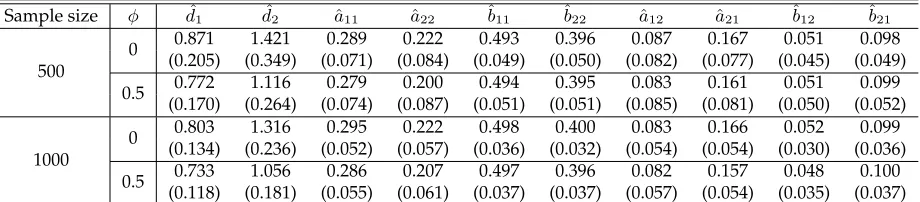
For the simulation study we only consider a two-dimensional process, that isp = 2. To initiate the max-imization algorithm, we obtain starting values for the parameter vectorθ = (d,vecT(A),vecT(B))as fol-lows. We first fit a univariate model to each series by using the methods of [21] and [20]. Then, employing the univariate predictions obtained from each of the hidden process, we run a multivariate linear regres-sion model by regressing the response to its lagged value and the vector of estimated hidden process. This method seems to work well in practice but further experiments are needed. Throughout the simulations we generate 1000 realizations with sample sizes of 500 and 1000 by employing the Clayton copula. We re-port the estimates of the parameters by averaging out the results from all simulations, and similarly, the standard errors correspond to the sampling standard errors of the estimates obtained by the simulation. Table1illustrates simulation results obtained from the linear model where the off-diagonal elements of the matricesAandBare non-zero, i.e. following parameters
A= 0.3 0.05
0.1 0.25
!
, B= 0.5 0.05
0.1 0.4
!
andd= (0.5,1). (18)
Note that these parameter values yieldk|A+Bk|2 = 0.89< 1butk|Ak|1+k|Bk|1 = 1(compare
Propo-sitions3.1and3.2). The empirical results largely agree with the theoretical properties of the estimators for both values of the copula parameterφwith the exception ofdˆ which does not approach normality satisfac-torily, but the approximation improves for larger sample sizes. Further simulation results are given in the supplement.
Sample size φ dˆ1 dˆ2 ˆa11 ˆa22 ˆb11 ˆb22 ˆa12 ˆa21 ˆb12 ˆb21
500
0 0.871 1.421 0.289 0.222 0.493 0.396 0.087 0.167 0.051 0.098 (0.205) (0.349) (0.071) (0.084) (0.049) (0.050) (0.082) (0.077) (0.045) (0.049)
0.5 0.772 1.116 0.279 0.200 0.494 0.395 0.083 0.161 0.051 0.099 (0.170) (0.264) (0.074) (0.087) (0.051) (0.051) (0.085) (0.081) (0.050) (0.052)
1000
0 0.803 1.316 0.295 0.222 0.498 0.400 0.083 0.166 0.052 0.099 (0.134) (0.236) (0.052) (0.057) (0.036) (0.032) (0.054) (0.054) (0.030) (0.036)
[image:14.612.81.541.482.583.2]0.5 0.733 1.056 0.286 0.207 0.497 0.396 0.082 0.157 0.048 0.100 (0.118) (0.181) (0.055) (0.061) (0.037) (0.037) (0.057) (0.054) (0.035) (0.037) Table 1. Simulation results for the multivariate linear model (1) by employing the Clayton copula with parameterφ. True parameter
5.2. Real data analysis
As an illustration of this methodology, we fit the linear and log-linear models to a bivariate count time series which consists of the number of transactions per 15 seconds for the stocks Coca-Cola Company (KO) and IBM on September 19th 2005. The data are from the NYSE Trade and Quote (TAQ) database, that contains intraday transactions data for all securities listed on the New York Stock Exchange (NYSE). It is of interest to study how two heavily traded stocks in different sectors, influence each others trading activity. There are 1440 observations in each of the two series, covering trades from 09:30 to 16:30, excluding the first 15 minutes and last 15 minutes of transactions. We remove these data, because transaction counts (and all other measures of intraday activity such as, e.g., volume) are typically characterized by a U-shaped diurnal seasonality (more transactions at the open and close and less at midday), which can interfere with the measurement of auto- and cross-correlations, see, e.g. [32].
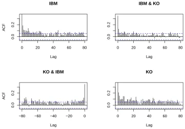
Figure1shows a time series plot of the data and Figure2depicts the autocorrelation function and cross-autocorrelation functions. Clearly, the plot of the cross-autocorrelation functions reveals high correlation within and between the individual transaction series. Note further that mean number of transactions is 4.854 and 4.276, for IBM and KO stocks, respectively. The sample variances are 13.809 (IBM) and 10.707 (KO), that is the data clearly shows marginal overdispersion.
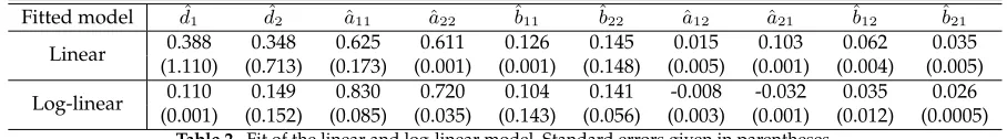
Table2shows estimated parameters after fitting the linear and log-linear models to these data. In both cases, the standard errors given in parentheses under the estimated parameters in Table2were computed using the robust estimator of the covariance matrix given byHn(θˆ)−1Gn(θˆ)Hn(ˆθ)−1whereHnandGnare given in equation (13) and (14), respectively. The magnitude of the standard errors shows that the feedback process should be considered in both models.
Fitted model dˆ1 dˆ2 ˆa11 aˆ22 ˆb11 ˆb22 ˆa12 ˆa21 ˆb12 ˆb21
Linear 0.388 0.348 0.625 0.611 0.126 0.145 0.015 0.103 0.062 0.035 (1.110) (0.713) (0.173) (0.001) (0.001) (0.148) (0.005) (0.001) (0.004) (0.005)
[image:15.612.81.535.437.500.2]Log-linear 0.110 0.149 0.830 0.720 0.104 0.141 -0.008 -0.032 0.035 0.026 (0.001) (0.152) (0.085) (0.035) (0.143) (0.056) (0.003) (0.001) (0.012) (0.0005)
Table 2. Fit of the linear and log-linear model. Standard errors given in parentheses.
The predictions from both models are denoted by Yˆi,t = λi,t(ˆθ) for i = 1 and 2, and are shown in Figure1. We see that the predictions approximate the observed processes reasonably well. We compare the two models by calculating the RMSE using the predictionsYˆi,t fori = 1and2for both models. This gives an RMSE of 190.06for the linear model and 193.25 for the log-linear model, indicating in total a better fit using the linear model. To examine the model fit, we consider the Pearson residuals, defined by
ei,t = (Yi,t−λi,t)/
p
0
10
20
30
40
Time
Transactions per 15 seconds (IBM) 09:45 11:45 14:00 15:30
0
5
10
15
20
Time
Transactions per 15 seconds (K
O)
[image:16.612.148.452.116.245.2]09:45 11:45 14:00 15:30
Figure 1: Number of transactions per 15 seconds for IBM (top) and Coca-Cola (bottom) and the respective predicted number of transactions from the linear model (red lines) and log-linear model (green lines).
0 20 40 60 80
0.0
0.2
Lag
A
CF
IBM
0 20 40 60 80
0.0
0.2
Lag IBM & KO
−80 −60 −40 −20 0
0.0
0.2
Lag
A
CF
KO & IBM
0 20 40 60 80
0.0
0.2
Lag KO
[image:16.612.120.481.324.576.2]0.0 0.1 0.2 0.3 0.4 0.5
0.0
0.2
0.4
0.6
0.8
1.0
frequency
0.0 0.1 0.2 0.3 0.4 0.5
0.0
0.2
0.4
0.6
0.8
1.0
frequency
0.0 0.1 0.2 0.3 0.4 0.5
0.0
0.2
0.4
0.6
0.8
1.0
frequency
0.0 0.1 0.2 0.3 0.4 0.5
0.0
0.2
0.4
0.6
0.8
1.0
[image:17.612.235.414.105.289.2]frequency
Figure 3: Left: Cumulative periodogram plots of the Pearson residuals from the linear fit of IBM (top) and Coca-Cola (bottom). Right: Cumulative periodogram plots of the Pearson residuals from the log-linear fit of IBM (top) and Coca-Cola (bottom).
both models, and examine their cumulative periodograms. Figure3supports the marginal whiteness of the residual process. A log-linear model that includeslog(Yt−1+c1p)for some constantc >1could had been entertained for modelling these data. However, predictions obtained after fitting such model for various values ofcdid not alter our results considerably (see also [23, p.571] for the univariate case). Finally, the results of the copula estimation, for this data example, are reported in the supplement.
Acknowledgements
Appendix
It is easy to see thatλ? = (I−A)−1dis a fixed point of the skeleton (3). The proof of the following lemma
is quite analogous to the proof of [21, Lemma A.1] and it is omitted.
Lemma A-1. Let{λt}be a Markov chain defined by (4) or (5). Ifk|Ak|2<1, then every point in[λ?1,∞)×
· · · ×[λ?
p,∞)is reachable, whereλ?i denotes thei’th component of the vectorλ ?
.
A-1. Proof of Proposition
3.1
The conditions ofφ-irreducibility and the existence of small sets can be proved along the lines of the proof of [21, Prop. 2.1] provided thatk|Ak|2<1. As in the proof of that Proposition we use the Tweedie criterion
to prove geometric ergodicity. Define now the test functionV(x) = 1 +kxkr
2. Then, we obtain asλi → ∞,
i= 1,2, . . . , p,
E
V(λmt )|λmt−1=λ
= 1 +E
kd+Aλ+BYtm−1+t;mkr2
∼ E
kAλ+BYmt−1k22
µ
,
where we assume, without loss of generality, thatµ=r/2,ra positive integer. Next,
E
kAλ+BYmt−1kr 2
=E
" hXp
i=1
(Aλ)i+ (BYmt−1)i
2i #µ
:=E
p
X
i=1
Ci
!µ
,
where(Aλ)iand(BYmt−1)iare theith components of the vectorsAλandBYmt−1, respectively. But
p
X
i=1
Ci
!µ
=X
i1
. . .X
ip
µ!
i1!. . . ip!
Ci1 1 . . . C
ip p ,
where the sum extends over all indices ij, j = 1,2, . . . p such that Ppj=1ij = µ. Successive use of the Cauchy-Schwartz inequality yields
E Ci1 1 . . . C
ip p
≤E1/2l1(C2i1l1 1 ). . .E
1/2lp(C2iplp p ),
where1≤lp≤2p−2, and
EC2iklk k
=E
(Aλ)k+ (BYmt−1)k4iklk
=E
4iklk
X
j=0
4i
klk
j
(Aλ)jk(BYt−1)4iklk−j
k
.
But using the reasoning on page 26 of [22], asλk→ ∞,k= 1, . . . , p,
Eh(BYt−1)4iklk−j
k |λt−1=λ
i
∼(Bλ)4iklk−j
Hence E1/2lkC2iklk k
∼((A+B)λ)2ik
k ,and asymptotically E
Ci1 1 . . . C
ip p
≤((A+B)λ)2i1
1 . . .((A+B)λ) 2ip p . Therefore we obtain that
E p
X
i=1
Ci
!µ
≤ X
i1
. . .X
ip
µ!
i1!. . . ip!
h
((A+B)λ)21i
i1
. . .h((A+B)λ)2pi ip
=
p
X
j=1
((A+B)λ)2j
µ
= k|(A+B)λk|2
2
µ
≤ k|(A+B)k|2 2kλk
2 2
µ
which, using the Tweedie criterion as in [21, Prop. 2.1], implies thatk|A+Bk|2<1is a sufficient condition,
and the proposition thus holds.
A-2. Proof of Lemma
3.1
To prove the first item of the Lemma, note that
kE(λmt −λt)k2 = kAE(λmt−1−λt−1) +BE(Ymt−1−Yt−1) +E(mt )k2
= kAE λmt−1−λt−1
+BhEhE(Ytm−1|FtY−,1;λm)i−EhEYt−1|F
Y,λ t−1
ii
+E(mt )k2
≤ k|A+Bk|2kE(λmt−1−λt−1)k2+kE(mt )k2,
whereFtY−,1λandF
Y,λ
t−1;mare theσ-algebras generated by{λs, s ≤ t}and{λms, s ≤ t}, respectively. By recursion and the fact thatkE(mt )k2 ≤cmwhich tends to zero asm→ ∞we obtain the desired result. To prove the second statement, note that asm→ ∞,
Ek(λmt −λt)k2
2 ∼ EkA(λ m
t−1−λt−1) +B(Ytm−1−Yt−1)k22.
Let∆t−1λ=λmt−1−λt−1and∆t−1Y=Ytm−1−Yt−1, then
Ek(λmt −λt)k2
2 ∼ E
h
∆t−1λTATA∆t−1λ+ ∆t−1λTATB∆t−1Y+ ∆t−1YTBTA∆t−1λ+ ∆t−1YTBTB∆t−1Y
i
= Eh∆t−1λTC∆t−1λ+ ∆t−1λTD∆t−1Y+ ∆t−1YTDT∆t−1λ+ ∆t−1YTE∆t−1Y
i
:= p
X
i=1 p
X
j=1
E[cij∆t−1λi∆t−1λj+dij∆t−1λi∆t−1Yj+dji∆t−1λi∆t−1Yj+eij∆t−1Yi∆t−1Yj],
whereC=ATA,D=ATBandE=BTB. By using properties of conditional expectation as before, we obtain
In addition, following the proof in [21, Lemma 2.1], and using the above conditioning argument, E ∆t−1Yi2
= E(∆t−1λi)
2
+ 2δi,m,whereδi,m → 0, asm → ∞. For the cross-terms we have to condition on the copula structure,FtY−,1;λm, as well i.e.
E(∆t−1Yi∆t−1Yj) = E
h
Eh∆t−1Yi∆t−1Yj|FtY−,1;λm,F
Y,λ t−1
ii
=E(∆t−1λi∆t−1λj).
Collecting all previous results, we obtain
Ek(λmt −λt))k2
2=Ek(A+B)(λ m
t−1−λt−1)k22+Dm≤ k|A+Bk|22Ek(λ m
t−1−λt−1)k22+Dm,
whereDm → 0asm → ∞. The last two statements are proved using straightforward adaptation of the proof of [21, Lemma 2.1].
A-3. Proof of Proposition
3.2
The proof is based on [17, Thm. 3.1] and parallels the proof given by [15]. In proving weak dependence, we define theXt= (YTt,λ
T
t)T and we employ the normkxk=kyk1+kλk1, whereis not necessarily small.
Then, the contraction property is verified by noting thatXt =F(XTt−1,N T
t)whereNtis an iid sequence ofp-variate copula Poisson processes and choosing=k|Ak|1/k|Bk|1. This proves that E[kYtk1]<∞and
E[kλtk1]<∞.
To show finiteness of moments we will be using induction and a different technique than the method used in [15]. More precisely, suppose that E[kYtkrr−−11]<∞and E[kλtkrr−−11]<∞forr∈Nandr >1. Then
consider thei-th component ofYt. But
EhYi,tr |FtY−1,λi ≤ Eh(Yi,t)r|FY ,λ t−1
i
+ r−1
X
k=1
|δik(r)|E
h
Yi,tk |FtY−1,λi
= λri,t+
r−1
X
k=1
|δik(r)|EhYi,tk |FtY−1,λi,
where(x)r=x(x−1)....(x−r+ 1),{δjk(r), k= 1,2, . . . , r−1}are some constants and the first line follows from properties of(x)rwhile the second line follows form properties of the Poisson distribution. By taking expectations and using thecr-inequality, we obtain that
E1/rhYi,tr
i
≤ E1/rhλri,t
i
+ r−1
X
k=1
|δik(r)|1/rµ i,
whereµi= maxk<rE
h
Yk i,t|F
Y,λ t−1
i
, which exists by the induction hypothesis. But
because of the properties of the linear model. Therefore, we obtain that (because of (3))
E1/r[Yi,tr]≤di+ p
X
j=1
aijE1/r[Yi,tr] + p
X
j=1
bijE1/r[Yi,tr] + r−1
X
k=1
|δik(r)|1/rµ i,
and by summing up, using the definition ofk|.k|1and its properties, we obtain that
p
X
i=1
E1/r[Yi,tr]≤ p
X
i=1
di+ (k|Ak|1+k|Bk|1) p
X
i=1
E1/r[Yi,tr] + p
X
i=1 r−1
X
k=1
|δik(r)|1/rµ i.
A-4. Proof of Lemma
3.2
We will prove the second and fourth conclusion as the other results follow from [23] and the proof of Lemma3.1. But to prove the second statement, note that
Ek(νmt −νt)k2
2 = EkAE(ν m
t−1−νt−1) +BE(log(Ytm−1+1p)−log(Yt−1+1p)) +E(mt )k
2 2
≤ k|Ak|2 2Ekν
m
t−1−νt−1k22+k|Bk| 2
2Eklog(Y m
t−1+1p)−log(Yt−1+1p)k22
+ 2k|Ak|2k|Bk|2
q
Ekνm
t−1−νt−1k22Eklog(Ymt−1+1p)−log(Yt−1+1p)|22+κc 2 m,
whereκ >0. Consider now the E(log(Ym
j,t−1+ 1)−log(Yj,t−1))2,j = 1,2, . . . , p. Then, following the proof
of [23, Lemma 2.1] and assuming without loss of generality thatλmj,t−1 ≥ λj,t−1we obtain that((Yj,tm−1+ 1)/(Yj,t−1+ 1)≥1. Therefore by using Jensen’s inequality (by employing the function(logx)2) we obtain
that
E
logY
m j,t−1+ 1
Yj,t−1+ 1
2
≤
"
logE
Ym
j,t−1+ 1
Yj,t−1+ 1
2#
.
But according to [23, p. 576] the right hand side of the above inequality is bounded by E(νm
j,t−1−νj;t−1)2
forj = 1,2, . . . , p. Hence, the conclusion of the Lemma follows again by the same arguments used in the proof of Lemma3.1.
To prove the fourth result, we follow [23, pp. 576-577]. Consider the test functionV(x) = exp(rkxk2)for
r∈N. Setb=rk|Bk|2. Then
E[exp(rkνmt k2)|νmt−1=ν] ≤ exp(r(kdk2+k|Ak|2kνk2))E[exp(rk|Bk|2klog(Ymt−1+1p)k2)|νmt−1=ν].
However
Ehexpbklog(Ytm−1+1p)k2
|νmt−1=νi = E
(
exphb
p
X
i=1
log2(Yi,tm−1+ 1)
1/2i
|νmt−1=ν
)
= E
(
exphb
p
X
i=1
νi+
log(Yi,tm−1+ 1)
exp(νi)
21/2
|νmt−1=ν
)
But
VarhY m t + 1
exp(νi)
|νmt−1=νi= exp(−νi)→0, (A-1)
provided thatνi→ ∞for alli= 1,2, . . . , p. Therefore we have that
VarhlogY m t + 1
exp(νi)
|νmt−1=νi→0,
by the delta-method for moments and provided thatνi→ ∞for alli= 1,2, . . . , p. Using now the multivari-ate delta-method and Cauchy-Schwartz inequality to the functiong(x1, . . . , xp) = exp(b(P
p
i(νi+xi)2)1/2) (with some abuse of notation), we obtain that
Var
(
exphb
p
X
i=1
νi+
log(Yi,tm−1+ 1)
exp(νi)
21/2
|νmt−1=ν
)
→0.
However
EhY m t + 1
exp(νi) |ν
m t−1=ν
i
∼1 (A-2)
provided thatνi→ ∞for alli= 1,2, . . . , p. Therefore, asymptotically, we obtain that
Ehexpbklog(Ymt−1+1p)k2
|νmt−1=νi∼exp(bkνk2).
To complete the proof, we note that the above calculations show that
Ehexp(rkνmt k2)|νmt−1=ν]≤exp(r(k|A2k|2+k|B2k|2−1)kνk2) exp(rkνk2).
Therefore, the conclusion follows as in [23, pp. 576-577].
A-5. Proof of Proposition
3.4
For the log-linear model we prove weak dependence by the following method. SetYj,t =Nj,t(exp(νj,t)),
j = 1,2, . . . , p. Then settingZj,t = log(1 +Yj,t)we have forXt = (Zt,νt)withZt = (Zj,t, j = 1,2, . . . , p) andNt= (Nj,t, j= 1,2, . . . , d)that
Xt= (Zt,νt) =F(XTt−1,N T t),
whereNt= (Nj,t, j = 1,2, . . . , p)iid copulap-variate Poisson processes. Then using again the same argu-ments as in [15] we obtain (with the same norm) that
E[kF(x,N)−F(x?,N)k] ≤
p
X
j=1
kA(ν−ν?) jk1+
p
X
j=1
kB(ζ−ζ?) jk1
+ kA(ν−ν?)k1+kB(ζ−ζ?)k1
≤ (1 +)k|Ak|1kν−ν?k1+k|Bk|1kζ−ζ?k1
where the first inequality follows from [23, pp.575–576]. The results now follow as in [15]. Now we show existence of moments for the log-linear model. Suppose thatr∈N. Then
E[exp(rkνtk1)|νt−1=ν] ≤ exp(r(kdk1+k|Ak|1kνk1))E[exp(rk|Bk|1kZt−1k1)|νt−1=ν]
Withb=rk|Bk|1, for the second factor of the right hand side we obtain that
EhexpbkZt−1k1
|νt−1=ν
i
= exp(bkνk1)E
hYp
i=1
Yi,t−1+ 1
exp(νi)
b
|νt−1=ν
i
But from the proof of Lemma3.2(see eq. (A-1)) and using similar arguments
Varh p
Y
i=1
Yi,t−1+ 1
exp(νi)
b
|νt−1=ν
i
→0,
provided thatνi → ∞, for alli= 1,2. . . , p. In addition, because of (A-2) and the multivariate delta-method of moments
Eh p
Y
i=1
Yi,t−1+ 1
exp(νi)
b
|νt−1=ν
i
→1,
provided thatνi→ ∞, for alli= 1,2. . . , p. The above two displays show that
EhexpbkZt−1k1
|νt−1=ν
i
∼exp(bkνk1),
as required.
A-6. Proof of Lemma
4.1
In what follows we drop notation that depends onθbecause all quantities are evaluated at the true param-eterθ0. The notationCrefers to a generic constant. Initially, we show that
∂λmt
∂dT −
∂λt
∂dT
2
< γm, a.s, (A-3)
for some positive sequenceγm→0, asm→ ∞. Using the first equation of (12) we obtain that
∂λmt
∂dT −
∂λt
∂dT
2 ≤ k|Ak|2
∂λmt−1
∂dT −
∂λt−1
∂dT
2
and therefore, by repeated substitution, (A-3) follows sincek|Ak|2 <1and the results of Lemma3.1.
Simi-larly,
∂λmt
∂vecT(A)−
∂λt
∂vecT(A)
Indeed, using the second equation of (12), we obtain that
∂λmt
∂vecT(A)−
∂λt
∂vecT(A)
2 ≤ √
pkλmt−1−λt−1k2+k|Ak|2
∂λmt−1
∂vecT(A)−
∂λt−1
∂vecT(A)
2,
where the first bound comes from the fact that in terms of the Frobenius matrix normk|Ipk|F =
√
p. There-fore, by Lemma3.1we obtain the desired result. Finally, it can be shown quite analogously (by using again Lemma (3.1)) that
∂λmt
∂vecT(B)−
∂λt
∂vecT(B)
2≤γm, a.s. (A-5)
To prove the lemma, we consider thed×dmatrix difference
s m t (s
m t )
T −s tsTt
2 = (s m
t −st)(smt ) T +s
t(smt −st)T
2
≤ ksmt −stk2k(smt ) Tk
2+kstk2k(smt −st) Tk
2. (A-6)
But
smt −st =
h∂λm
t
∂θT
T
−∂λt
∂θT
Ti
Dmt
−1
Ymt −λmt
+ ∂λt
∂θT
Th
Dmt
−1
−Dt
−1i
Ymt −λmt
+ ∂λt
∂θT
T
D−t1
h
Ymt −λ m t
−Yt−λt)
= (I) + (II) + (III), (A-7)
with obvious notation. Then we obtain for the first term(I)of (A-7)
kh∂λ
m t
∂θT
T
−∂λt
∂θT
Ti
Dmt
−1
Ymt −λ m t
k2 ≤
∂λmt
∂θT −
∂λt
∂θT
2
Dmt
−1 2k
Ymt −λ m t
k2.
(A-8)
We deal with the first factor. Recall thatk|.k|F stands for the Frobenius norm of a matrix. Then
∂λmt
∂θT −
∂λt
∂θT
2 2 ≤
∂λmt
∂θT −
∂λt
∂θT
2 F =
∂λmt
∂dT −
∂λt
∂dT
2 F +
∂λmt
∂vecT(A)−
∂λt
∂vecT(A) 2 F+
∂λmt
∂vecT(B)−
∂λt
∂vecT(B)
2 F ≤ p
∂λmt
∂dT −
∂λt
∂dT
2 2
+p2
∂λmt
∂vecT(A)−
∂λt
∂vecT(A)
2 2
+p2
∂λmt
∂vecT(B)−
∂λt
∂vecT(B)
2 2 ,
where the first and third inequality hold because of result 4.67(a) of [51] and the second inequality is a consequence of the definition of Frobenius norm. Then we need to show that
Eh
∂λmt
∂dT −
∂λt
∂dT
2 2 i
, Eh
∂λmt
∂vecT(A)−
∂λt
∂vecT(A)
2 2 i
, Eh
∂λmt
∂vecT(B)−
∂λt
∂vecT(B)
2 2 i
withγm→0. We deal with the middle term only; similar arguments can be used for the other two terms. Squaring the expression after (A-4) and taking expectations we obtain that
Eh
∂λmt
∂vecT(A)−
∂λt
∂vecT(A)
2 2 i
≤ pEhkλmt−1−λt−1k22
i
+k|Ak|22E
h
∂λmt−1
∂vecT(A)−
∂λt−1
∂vecT(A)
2 2 i
+ 2√pk|Ak|2E
h
kλmt−1−λt−1k2
∂λmt−1
∂vecT(A)−
∂λt−1
∂vecT(A)
2 i
≤ δ2;m+k|Ak|22E
h
∂λmt−1
∂vecT(A)−
∂λt−1
∂vecT(A)
2 2 i
+ 2C√pk|Ak|2
p
δ2;m≤γm,
whereγmcan become arbitrarily small. This follows from Proposition3.1, (A-4) and the fact thatk|Ak|2<1.
For the second term of (A-8) we note that
Dmt
−1 2≤ s p max 1≤i≤p
1
d2 i
≤C, (A-10)
wherediis thei’th component ofd. In addition
EhkYmt −λmt k2 2 i = p X i=1
E[λmi,t]< C (A-11)
by Proposition3.1and using a conditioning argument. Collecting (A-9), (A-10) and (A-11) an application of Cauchy-Schwartz inequality shows that the
Eh
∂λmt
∂θT −
∂λt
∂θT
2
Dmt
−1 2k
Ymt −λmt k2
i
→0,
asm→ ∞. Now we look at the second summand(II)of (A-7). First of all, we note that E ∂λt/∂θ
T 4
2< C.
This is proved by using the same decomposition of the norm as the sum of norms of the matrix of deriva-tives with respect tod,vec(A)andvec(B). Then using (12), the fact that
A
2<1and the compactness
of the parameter space, the result follows. In addition, for some finite constants(cij), we obtain that
EhkYmt −λmt k4 2
i
= Eh
p
X
i=1
(Yi,tm−λmi,t)2
2i
= Eh
p
X
i=1
(Yi,tm−λmi,t)4+ 2X
i6=j
(Yi,tm−λmi,t)2(Yj,tm−λmj,t)2i
≤
p
X
i=1
E[(λmi,t)4] + p X i=1 3 X j=1
because of Proposition3.1and from the same arguments given in the proof of Proposition 3.2. Now we have that
Dmt
−1
−Dt
−1
2
2 ≤Ckλ m t −λtk22
and therefore its expected value tends to zero by Lemma3.1. Collecting all these results we have that the expected value of(II)in (A-7) tends to zero. Finally, the expected value of term(III)in (A-7) tends to zero, asm→ ∞by combining the above results and using Cauchy-Schwartz inequality and Lemma3.1.In addition, the above results show that E[kstk22]<∞. The conclusion of the Lemma follows.
References
[1] A. Ahmad. Contributions `a l’´econem´etrie des s´eries temporelles `a valeurs enti`eres. PhD thesis, University Charles De Gaulle-Lille III, France, 2016.
[2] A. Ahmad and C. Franq. Poisson QMLE of count time series models. Journal of Time Series Analysis, 37:291–314, 2016.
[3] C. M. Andreassen. Models and inference for correlated count data. PhD thesis, Aaarhus University, Den-mark, 2013.
[4] D. Andrews. Non-strong mixing autoregressive processes. Journal of Applied Probability, 21:930–934, 1984.
[5] I. V. Basawa and B. L. S. Prakasa Rao. Statistical Inference for Stochastic Processes. Academic Press, London, 1980.
[6] T. Bollerslev. Generalized autoregressive conditional heteroskedasticity.Journal of Econometrics, 31:307– 327, 1986.
[7] V. Christou and K. Fokianos. Quasi-likelihood inference for negative binomial time series models. Journal of Time Series Analysis, 35:55–78, 2014.
[8] D. R. Cox. Statistical analysis of time series: Some recent developments.Scandinavian Journal of Statis-tics, 8:93–115, 1981.
[9] R. A. Davis, W. T. M. Dunsmuir, and Y. Wang. On autocorrelation in a Poisson regression model. Biometrika, 87:491–505, 2000.
[10] R. A. Davis and H. Liu. Theory and inference for a class of observation-driven models with application to time series of counts.Statistica Sinica, 26:1673–1707, 2016.
[11] J. Dedecker, P. Doukhan, G. Lang, Jos´e R. Le ´on R., S. Louhichi, and C. Prieur. Weak dependence: with examples and applications, volume 190 ofLecture Notes in Statistics. Springer, New York, 2007.
[12] M. Denuit and P. Lambert. Constraints on concordance measures in bivariate discrete data. Journal of Multivariate Analysis, 93:40–57, 2005.
[14] R. Douc, K. Fokianos, and E. Moulines. Asymptotic properties of quasi-maximum likelihood estima-tors in observation-driven time series models.Electron. J. Stat., 11:2707–2740, 2017.
[15] P. Doukhan, K. Fokianos, and D. Tjøstheim. On weak dependence conditions for Poisson autoregres-sions.Statistics & Probability Letters, 82:942–948, 2012. with a correction in Vol. 83, pp. 1926-1927. [16] P. Doukhan and S. Louhichi. A new weak dependence condition and applications to moment
inequal-ities.Stochastic Processes and their Applications, 84:313–342, 1999.
[17] P. Doukhan and O. Wintenberger. Weakly dependent chains with infinite memory. Stochastic Processes and Their Applications, 118:1997–2013, 2008.
[18] B. Efron. Double exponential families and their use in generalized linear regression. Journal of the American Statistical Association, 81:709–721, 1986.
[19] R. Ferland, A. Latour, and D. Oraichi. Integer–valued GARCH processes.Journal of Time Series Analysis Analysis, 27:923–942, 2006.
[20] K. Fokianos. Statistical Analysis of Count Time Series Models: A GLM perspective. In R. Davis, S. Holan, R. Lund, and N. Ravishanker, editors,Handbook of Discrete-Valued Time Series, Handbooks of Modern Statistical Methods, pages 3–28. Chapman & Hall, London, 2015.
[21] K. Fokianos, A. Rahbek, and D. Tjøstheim. Poisson autoregression. Journal of the American Statistical Association, 104:1430–1439, 2009.
[22] K. Fokianos, A. Rahbek, and D. Tjøstheim. Poisson autoregression (complete vesrion). 2009. available athttp://pubs.amstat.org/toc/jasa/104/488.
[23] K. Fokianos and D. Tjøstheim. Log–linear Poisson autoregression. Journal of Multivariate Analysis, 102:563–578, 2011.
[24] C. Francq and J.-M. Zako¨ıan. GARCH models: Stracture, Statistical Inference and Financial Applications. Wiley, United Kingdom, 2010.
[25] J. Franke and T. Subba Rao. Multivariate first-order integer values autoregressions. Technical report, Department of Mathematics, UMIST, 1995.
[26] C. Genest and J. Neˇslehov´a. A primer on copulas for count data. Astin Bull., 37:475–515, 2007.
[27] A. Heinen and E. Rengifo. Multivariate autoregressive modeling of time series count data using cop-ulas.Journal of Empirical Finance, 14:564 – 583, 2007.
[28] C. C. Heyde. Quasi-Likelihood and its Applications: A General Approach to Optimal Parameter Estimation. Springer, New York, 1997.
[29] H. Joe. Multivariate Models and Dependence Concepts. Chapman & Hall, London, 1997.
[30] N. L. Johnson, S. Kotz, and N. Balakrishnan. Discrete multivariate distributions. John Wiley, New York, 1997.
[31] B. Jørgensen, S. Lundbye-Christensen, P. X.-K. Song, and L. Sun. State-space models for multivariate longitudinal data of mixed types.The Canadian Journal of Statistics, 24:385–402, 1996.