Diagnosis and Resolution of Infeasibility in the Constraint Method for Solving Multi Objective Linear Programming Problems

Diagnosis and Resolution of Infeasibility in the Constraint

Method for Solving Multi Objective Linear

Programming Problems

Mohammadreza Safi, Hossein Zare Marzooni Department of Mathematics, Semnan University, Semnan, Iran Email: [email protected], [email protected]

Received September 18, 2011; revised October 20, 2011; accepted November 5, 2011

ABSTRACT

In this paper we discuss about infeasibility diagnosis and infeasibility resolution, when the constraint method is used for solving multi objective linear programming problems. We propose an algorithm for resolution of infeasibility, which is a combination of interactive, weighting and constraint methods. Numerical examples are provided to illustrate the tech-niques developed.

Keywords: Multi Objective Linear Programming; Weighting Method; Constraint Method; Infeasibility Analysis; IIS

1. Introduction

Almost every important real world problem involves more than one objective. The multi objective linear pro- gramming (MOLP) problem can be formulated as fol- lows:









, ,

. . : , 0

T k

s t    

c x

x X x Ax b x



, 1, ,

T _{j k}

c 

*

T T

i  i

c x c x T T *

l  l

c x c x

1 l k

POSs and for improving the previous methods [5-7].

proaches decision maker (D

ave discussed diagnosis of

e deletion filter and the elastic fil

for obtaining a PO

1 max z_{ c x}T

(1)

where j are n-dimensional vectors, x is an n-dimensional vector, b is an m-dimensional vector and

A is anm × n matrix.

Excluding the trivial case in which a point exists in the feasible region which maximizes all objectives simulta- neously, we must often propose a compromise solution to decision maker (DM). In the special case, the point that simultaneously maximizes all objectives is called com- plete optimal solution. In general, such point rarely exists. Thus, instead of complete optimal solution, Pareto opti- mal solution (POS) is introduced. x* _{is a POS for Prob-}

lem (1.1) if there does not exist another x such that for all i and for at least one .

There are several methods for solving the MOLP Problem (1). By the utility function method [1] we obtain a compromise solution. The weighting method proposed by Kuhn and tucker [2], the constraint method proposed by Haimes et al. [3] and the weighted minimax method proposed by Bowman [4], characterize POSs. Since then, many different approaches are developed for obtaining

Also, there are several fuzzy approaches for solving MOLP problems such as [7-9].

In all of the methods and ap

M) has an essential role. However, choosing unsuit- able bounds in the constraint method by DM may be oc- cur infeasibility in the problem.

Many published researches h

infeasibility, [1,10-13], however, there are few papers deal with infeasibility resolution [14-16]. One of the useful references is [17].

In this paper we use th

ter algorithms for isolating IIS (irreducible infeasible subsystems) in order to diagnose infeasibility. For resolu- tion of infeasibility and obtaining a POS, we propose analgorithm which is a combination of interactive, weight- ing and constraint methods. Also we recall the fuzzy method of Leon and Liern [14] for repairing the con-straint, in order to attain a feasible space.

Section 2 recalls the constraint method

2. Solving MOLP Problems

ing MOLP problems g the many possible

ble bounds is a pr

terizing POS is to solve d by taking one

objec-, 1, , :

There are several methods for solv and obtaining the POSs [1]. Amon

ways of scalarizing the MOLP, the weighting and the constraint methods are the most famous methods. In these methods DM should determine the weights and the bounds for every objective, respectively.

In this section we recall the constraint method. How-ever, determining good weights and suita

oblem for DM. Therefore, we propose a combination method of the weighting and the constraint method.

2.1. The Constraint Method The constraint method for charac the constraint problem formulate

tive as the objective function and letting all the other objective functions be inequality constraints. The con-straint problem is defined by

max . . ε

T j T

,

i i

s t  i 

x X

re εi, i = 1, ···, k; i j; are chose

k i j

 (2)

whe n by DM.

If is a unique optimal solution to Problem (2)

k; i to

Prob-le 1). C

tion o

r some inconsistency quent is

c x c x

*_

x X

for some εi, i = 1, ···,  j then x* is a POS

m ( versely, If _x*_{X is a POS of Problem (1),}

then x* _{is an optimal solu f the Problem (2) for some}

εi, i = 1, ···, k; i j.

Set



: T , 1, , : , 0



i i i k i j

     

S x c x ε x . Choos-

ing unsuitable on

εi by DM may occu

in the constraints and its conse   or   

S X even though S  and X . This in-consistency follows the infeasibility in the prob

focus on the ob es, we s only the case S , and suppose that, after repairing S an

S

lem. Here for jectiv discus

d at-ta

omb thod

for some objectives, ctives he or she hasn’t ining S  we have S  X .

2.2. A C ination Me

Sometimes, DM has suitable bounds tentatively, but for the other obje

any assessment. Similarly, in weighting method, it’s pos- sible, DM has some weights for comparison of some objectives together, but he or she doesn’t know how to appropriate some weights for the other objectives. In this case the combination of the two methods may be useful.

Consider Problem (1). Suppose DM has some good weights wi 0,i J 1 for comparison of 1

T i i J

c x and some suitable lower bounds  i,i J2for , 2

T i i J

c x ,

where



J J₁, ₂



k . We S:

2

. .T ,

i i

is a partition for



1, 2, ,



solve the following problem in order to PO

1

max T

i i i J

z w

 



c x

obtain a

tc x i . (3)

s J



x X

Theorem 2.1. If Problem (3) has a u

lutionx*_{, thenx}*_{is a POS for Problem (1)}nique optimal so-_.

Proof:Let (contrary) x*_{be inefficient, then there exist} x X , such that _cT _cT *

ix ix for all i J 1;

*

cT _cT i 

x x , for all i J₂

i  ;

*

T T

c_txc_tx , for some i J ₁

or some i J₂

or f  . Thus

1

*

i i

i J  1

T T

i i i J

w _ w



c x



c

contradiction to unique optimality of x*_.

_

irreducible

in-[18]. An IIS has

till infeasible, go to step 1).

3.

The deletion filter proposed by Chinneck and Dravnieks ation of exactly one IIS after

he set.

x ,

3. Diagnosis of the Infeasibility

All infeasible systems have one or more

feasible subsystems (IISs) of constraints

the property that it is itself infeasible, but any proper subsystem is feasible. An infeasible set of constraints can be rendered feasible by deleting or repairing at least one member of every IIS it contains. Finding the smallest cardinality set of constraints to cover all IISs is known as the minimum-cardinality IIS set-covering problem (MIN IIS COVER) [19].

There are several practical issues related to IIS isola-tion. An excellent summary of the recently developed algorithmic methods has appeared in [17]. Here we recall

the deletion filter and the elastic filter. The deletion filter guarantees the identification of exactly one IIS, but the exiting of the elastic filter is a small infeasible set that is not necessarily an IIS, but it has at least one IIS.

If the number of objectives in Problem (1) is small, it’s better we use deletion filter. Else, we use elastic filter and then use deletion filter on the exiting of elastic filter for obtaining an IIS.

It may be that there are multiple infeasibilities in the model, hence IIS isolation typically is used in a cyclic manner

1) Isolate an IIS;

2) Determine a repair for this IIS; 3) If the model is s

1. The Deletion Filter

[18] guarantees the identific

a single pass through the set of constraints. This is an essential property possessed by very few of the IIS isola-tion methods. In the following algorithm, for diagnosis infeasibility of the problems, we use the phase I of the simplex method.

INPUT: an infeasible set of constraints.

For each constraint in the set:

1) Temporarily drop the constraint from t

IF feasible THEN return dropped

s constituting a single IIS.

rns exactly one II

The Elastic Filter

Th ally described by Brown and Graves adds nonnegative elastic vari- and minimizes the summation

constraint to the set.

ELSE(infeasible) drop the constraint permanently.

OUTPUT: constraint

Theorem 3.1: The deletion filter retu S.

Proof: See [18].

3.2.

e method origin

[20]. A fully elastic program ables ei to every constraint

of these variables as an elastic objective function. This allows finding a feasible solution for the original infeasi-ble model. Namely we solve the following proinfeasi-blem:

1 min k i

i i j

e e

 



_

. .T ,

i i i 1, , ;

s tc x e ε i k i j, (4)

1, , ;k i j

   .

m are shown in ing:

INPUT: an infeasible set of constraints

tive elastic variables ei.

tive function.

oving, Go to step 2.

4.

asibility analysis is the lem to make it ches and prac-

l

prob IIS COVER). There are several algo-

he number of co

ve the Problem, (4):



0,e_i 0,i

 

x

The details of the algorith the follow-

.

1) Make all constraints elastic by incorporating non-

nega

2) Solve the model using the elastic objec

3) IF feasible THEN enforce the constraints in which any ei> 0 by permanently rem

ELSE(infeasible)Exit.

OUTPUT: the set of de-elasticized enforced con- straints contains at least one IIS.

Resolution of the Infeasibility

The second major aspect of infe

infeasibility resolution to repair the prob feasible. However, most published resear

tice results in recent years have focused on the diagnosis side. Little investigation has been made in infeasibility resolution [13,14,16].

4.1. Resolution of Infeasibility in the Constraint Method

The smallest cardinality set of constraints to cover al IISs is known as the minimum-cardinality IIS set-covering

lem (MIN

rithms for finding MIN IIS COVER [17].

In this paper we concentrate on infeasibility in con- straint objectives. In almost all of real problems, the number of objectives is very less than t

nstraints. It is usual that in many problems, MIN IIS

COVER for the set of constraint objectives be singleton. For this special case our algorithm proposes an interac-tive method, and for the other cases we use the combina-tion method mencombina-tioned in Seccombina-tion 2.2 or the approach of Leon and Liern (Section 4.2) in order to repair the con-straints and resolve infeasibility. Besides, a POS is ob-tained.

The Combination Algorithm

Consider Problem (2): 1) Sol

2) Set I1



i e; i 0



, I2 



i e; i 0



,

3) If I2 , there is no infeasibility, solve Problem

(2) and STOP.

 

2

4) If I  t for some 1 t m t, j, and t = w,

th ever,

algorithm. Use Leon and Liern method

fo g Probl



en, how MIN IIS COVER is singleton, but there is

a cycling in the

r solvin em (2).

Else, If I₂ 

 

t for some 1 t m t,  j, and t ≠w,

then MIN IIS COVER is singleton, set w: = t, replace

T j

c x by T

t

c x in Problem (2), take εj from DM, change

the role of j and t in Problem (4) and go to Step 1. 5) If I2 2 and I1  then take w i Ii,  2

 

j

DM solve Problem (3), STOP.

6) If I1

from and

 , then use Leon and Liern method for

so roblem

roblem:

lving P (2).

Example 4.1 Consider the following p

1 2 3

min 3x 3x 3x

1 2 3

min 2x x 2x

1 2 3

min 4x 4x 2x

1 2 3

minx 6x 5x

1 2 3

. .4 2 4 1

s t x  x  x  8

1, ,2 3 0.

x x x 

Let DM chooses the first objective as the main and ε2

= 18, ε3 = 6, ε4 = 14 as the upper b und of the other

ob-jectives. So the problem of findi POS changes to so

o ng a lving the following problem:

1 2 3

min 3x 3x 3x

1 2 . .2 2

s t x x  x318

1 2 3

4x 4x 2x 6

1 6 2 5 3 24

x  x  x 

1 2 3

4x 2x 4x 18

1, ,2 3 0.

x x x 

The last problem is infeasible. By solving Problem (4) we obtain * *

2 4 0

e e  , but * 3

e  . Namely MIN IIS COVER is singleton. Thus we take 4x + 4x + 2x ≤ 14 as

blem is

0

1 2 3

the main objective. Suppose that DM chooses ε1 = 14.

1 2 3 min 4x 4x 2x

. .2 2 18

s t x₁x₂ x₃

1 23x314 16 25x324 1 2 4 3 18

x  x  x 

1, ,2 x30.

The last has the optimal solution



* * *



1, ,2 3 3x 3x

x x

4 2

x x

problem x x x

0, 0,

 POS fo oblem.



Example 4.2 Consider the fo em:



4.5



that is a r the main pr llowing probl

1 2 3

min 3x 3x 3x

1 2 3

min 2x 3x 2x

1 2 2 4 3 min 3x  x  x

1 2 2 3 maxx  x x

1 4 2 3 maxx  x x

13x24x3 1, ,2 3 0.

x x x 

objective as the main and ε2 =

6, e bounds of the other objec-tives.

. .2

s t x 2

Let DM choose the first ε3 = 6, ε4 = 8, ε5 = 9 as th

Solving Problem (3.1) leads to



* * *



1, ,2 3

x x x =



0, 2.25,0



and



* * * *







2, , ,3 4 5 0.75,0,3.5,0

e e e e  . Thus,

 

1 2, 4

I  and I2 

 

1,3 i.e. I1  and 2

Problem (2 = 0.3. Th

we ):

2

I  according to our algorithm, we must solve .2).

w1 erefore,

e follow roblem (2.2













1 2 3 1 2 3

1 2 3

min 0.5 3 3 3 0.2 2 3 2

0.3 2

Let DM choose = 0.5, have th ing num

w2 = 0.2, w4

erical form of P

x x x x x x x x x

    

   

1 2 3

. .3 2 4

s t x  x  x

1 4 2 3 9

x  x x 

6



1 24x32 1, ,2 x30.

The n



* * *



1, ,2 3 2x 3x

x x

optimal solution is agai x x x =

0,

4. ty by Fuz

osed by in order to resolve infeasibility.

3]. The method is stated as fol-lo

i i

, 1, , ; , 0

T

i i i k i j



2.25, 0



.



2. Resolution of Infeasibili zy Approach

In this section we recall the fuzzy method prop Leon and Liern [14] for repairing the constraints

The main idea is that the fuzzy membership function expresses the degree to which a particular point satisfies a given constraint. The membership function makes use

of Roodman’s limits [1 ws:

So as to obtain a feasible solution, let us reformulate the system

, 1, , ; , 0

T _{ i k i j }

c x ε  x , (5) As the fuzzy case

  

c xε  x (6) Assume that denote the fuzzy constraints b

C

y

, 1, , ;

i i  k i k an

 _{d their membership functions by}

, 1, , ;

i

C i k i k

    , respectively. The con the membership function by Roodman’s

ba (5) and

its dual (DPI). The

ε , 1, , ; , , , . . i I I i i k i j 0

s t

struction of approach is sed on Phase I problem (PI) associated System

se problems can be stated as follows:

(PI)

1 min k i

i i j r  



T _{     }

c x s r  x s r , where s

and r are surplus an l vectors, respectively.

(DPI)

1 max k πi i

i d artificia  i j 



1, , j i j s j   

where j, 1, ,

i

c j  n are the elements of T i

c . Let z* _{be the optimal value of (PI) and}

*

πi,i 1, , ;k i j



k

1

π 0,

. . i i ,

i c n t  



   , be the optimal solution of (DPI). Since system (5) is infeasible, then _z*_{0. For}

1, , ;

i  k i j set

* * π i i z p 

if _π* ₀

i  and pi = 0 if π*i 0. The values of pi s are called the Rood man lower bo onsid

ing membership function:

unds. C er the

follow-0 1 i i i T T i i

i i i i

C i p if p p         1 T i T i i if if _      x ε c x

ε c x ε

 (7)

 _



c

c x ε

for i1, , ; k i j.

Define the fuzzy set of feasible solutions (4.1) as

of system



( , _E

 

, n



E x x x R where



1



min , ,

k

E C C

    .

lu n s

en by

 



The so tio with the highe t degree of membership

E is giv





max arg max minx i C_i

So we solve the auxiliary crisp problem: (AP) min

. .

. j  α 1， 0

) has feasible

solu-tio nction

value.

Theorem 4.1. (AP) is feasible and its optimal value α*

a when w the constrain od for solving multi objective linear programming. We used el deletion nding IIS. We pro-p ation method for obtaining In the in airing the objectives, and for

and A. W. Tucker, “Nonlinear Program-ming,” In: J. Neyman, Ed., Proceeding of the 2nd Berke-ley Symposium stics and

Probabil-, 1, , ; , 0

T

i i i

stc xp ε i  k i The next theorem proves that (AP

x

n and provides a lower bound for objective fu

verifies that _1k*_{1, where k is the number of non-} null shadow prices of (PI).

Proof: see [14].

In fact β* _{= 1 – α}* _{is the degree of feasibility.}

Example 4.3. Consider Problem 4.2. Let DM choose the first objective as the main with the same value for the bounds of the other objectives. As mentioned in Example 4.2, the problem is infeasible.

* *

Solving (PI) and (DPI) lead to z = 4.25, 2 =1, *3

= 0, * 4

 = 1, * 5

 = 0.25. Therefore, p2 = 4.25, p3 = 0, p4

= 4.25, p5 = 17. So we must solve the following problem:

1 2 3

. . 2 3 2

s t  x  x  x

1 2 3

1 2 3

3 2 4 0 6

2 1 4.25 8

4 17 18

x x x x x x x x x

 

     

   

   

1 2 3

1, ,2 3 0

x x x 

4.25 6

  

The optim



*







3

,  0, 2. ,0 with α = 0.5647.



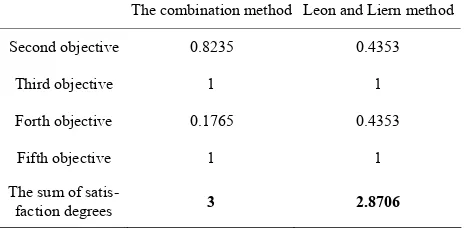
In order to compare the obtained solutions by two methods described in Examples 4.2 and 4.3, we compute the satisfaction degree of the objectives with th

[image:5.595.57.289.620.734.2]

ns (4.3). The results a

Table 1. A comparison between use of the combin on and Liern method in Examples 4.2

The combination method Leon and Liern method al solution is * *

1 2,

x x x 8 *

e mem-bership functions in equatio re sum-marized in the following Table 1.

According to Table 1, the summation of satisfaction degree in our algorithm is better than the Leon and Liern method, however, the minimum degree in the Leon and Liern method is better.

5. Conclusion

In this paper we discussed about infeasibility, diagnosis

ation method and the Le

and 4.3.

Second objective 0.8235 0.4353

Third objective 1 1

Forth objective

faction degrees 2.

0.1765 0.4353

Fifth objective 1 1

The sum of

satis-3 8706

nd resolution, e used t meth

astic filter and filter for fi osed a combin

terest of rep

POSs. constraint

resolution of infeasibility, we proposed an algorithm, which was a combination of interactive, weighting sum and constraint method. We solved some numerical ex-amples and compared our method with Leon and Liern method.

REFERENCES

[1] R. Steuer, “Multiple Criteria Optimization: Theory Com-putation and Application,” Wiley, New York, 1986. [2] H. W. Kuhn

on Mathematical Stati

ity, University of California Press, Berkeley, 1951, pp. 481-492.

Y. Y. Haimes, L. Lasdon and D. Wismer, “On a Bicr

[3] iteria

Formulation of the Problems of the Integrated System Identification and System Optimization,” IEEE Transac-tion on Systems, Man, and Cybernetics, SMC-1, No. 3, 1971, pp. 296-297.

V. J. Bowm

[4] an, “On the Relationship of the Tchebycheff Norm and the Efficient Frontier of Multi-Criteria Objec-tives,” In: H. Thiriez and S. Zients, Eds., Multiple-Crite- ria Decision Making, Springer-Verlag, Berlin, 1976, pp. 76-86.

[5] A. Arbel and P. Korhonen, “Using Aspiration Levels in an Interactive Interior Multi-Objective Linear Program-ming Algorithm,” European Journal of Operational Re-search, Vol. 89, No. 1, 1996, pp. 193-201.

[6] M. Zangiabadi, M. R. Safi and H. R. Maleki, “An Algo-rithm For Solving Multi Objective Programming Prob-lems,” Logic Colloquium, ASL, European Summer Meeting, Turin, 2004.

[7] H. J. Zimmermann, “Fuzzy Programming and Linear Programming with Several Objective Functions,” Fuzzy Sets and Systems, Vol. 1, No. 1, 1987, pp. 45-55. doi:10.1016/0165-0114(78)90031-3

[8] S. M. Guu and Y. K. Wu, “A Compromise Model for Solving Fuzzy Multi Objective Linear Programming Problems,” Journal of Chinese, Institute of Industrial En-gineers, Vol. 18, No. 5, 2001, pp. 87-93

[9] M. Jimenez and A. Bilbao, “Pareto Optimal Solutions in Fuzzy Multi Objective Linear Programming,” Fuzzy Sets and Systems, Vol. 160, No. 18, 2009, pp. 2714-2721. doi:10.1016/j.fss.2008.12.005

[10] N. Chakravarti, “Some Results Concerning Post-Infeasi-bility Analysis,” European Journal of Operational Re-search, Vol. 73, No. 1, 1994, pp. 139-143.

doi:10.1016/0377-2217(94)90152-X

doi:10.1016/0305-0548(94)90057-4

[12] J. W. Chinneck, “Fast Heuristics for the Max ble Subsystem Problem,” INFORMS

imum Journal on Com-puting,Vol. 13, No. 3, 2001, pp. 210-223.

doi:10.1287/ijoc.13.3.210.12632 [13] G. M. Roodman, “Post-Infeasibility

Programming,” Management Scienc

Analysis in Linear e, Vol. 25, No. 9, 1979, pp. 916-922. doi:10.1287/mnsc.25.9.916

[14] T. León and V. Liern, “A Fuzzy Method to Repair Infea-sibility in Linearly Constrained Problems,

and Systems, Vol. 122, No. 2, 200

” Fuzzy 1, pp. 237-243.

Sets doi:10.1016/S0165-0114(00)00010-5

[15] M. Tamiz, S. J. Mardle and D. F. Jones, “Detecting IIS in Infeasible Linear Programming Using Techniques from Goal Programming,” Computers and Operations Re-search, Vol. 23, No. 2, 1996, pp. 113-119.

doi:10.1016/0305-0548(95)00018-H

[16] J. Yang, “Infeasibility Resolution Based on Goal Pro-gramming,” Computers and Operations Research, Vol.

35, No. 5, 2008, pp. 1483-1493. doi:10.1016/j.cor.2006.08.006

[17] J. W. Chinneck, “Feasibility and Infeasibility in Optimi-zation. Algorithms and Computational Methods,” Springer, New York, 2008.

[18] J. W. Chinneck and E. W. Dravnieks, “Locating Minimal

.157

Infeasible Constraint Sets in Linear Programs,” ORSA Journal on Computing, Vol. 3, No. 2, 1991, pp. 157-168. doi:10.1287/ijoc.3.2

27-144.

[19] J. W. Chinneck, “An Effective Polynomial-Time Heuris-tic for the Minimum-Cardinality IIS Set-Covering Prob-lem,” Annals of Mathematics and Artificial Intelligence, Vol. 17, No. 1, 1996, pp. 1

doi:10.1007/BF02284627