Performance Evaluation of Neural Network and Deep
Neural Network for Human Activity Recognition
Dalia Khairy
Computer DepartmentDamietta University Egypt
Gamal Behery
Mathematical Dept. Damietta UniversityEgypt
A. A. Ewees
Computer DepartmentDamietta University Egypt
Elsaeed AbdElrazek
Computer DepartmentDamietta University Egypt
ABSTRACT
Human activity recognition (HAR) has given a lot of attention in the recent years due to the need of high level context about the human activities in several applications. Many domains have attempted to overcome the lack of performance techniques used to collect raw data such as cameras to record or capture activities and inertial sensor units to record correct readings. As a result, few studies have regarded to acquire raw data and extract features instead of understanding, recognizing, inferring, and predicting human activities in future to obtain recommendations or detecting healthcare, daily, and educational positions to humans. This paper aims to analyze the performance of Neural Network (NN) and Deep Neural Network(DNN) for HAR. To achieve this aim, we select Daily and Sports Activities data set (DSA) to match paper's needs. This paper depends on NN and DNN based on softmax function. We form three sets of DSA dataset: small, medium, and large. The results showed that DNN based on softmax function reduce the computational cost than NN, increase the performance of network, and achieved high overall successful differentiation rate in testing on large dataset (97.74%) than on medium dataset (67.81%). or on small dataset (67.63%).
Keywords
Human Activity Recognition(HAR), Neural Network(NN), Deep Neural Network(DNN)
1.
INTRODUCTION
Human activity recognition (HAR) is a field that focuses on monitoring and understanding the daily activities of humans via computational methods. There are two major methods are used to collect data in HAR: computer vision systems using cameras and systems used inertial sensors [1]. In computer vision, cameras have been used to capture images or record videos about human activities to enable recognizing and inferring them. Unfortunately, many humans dislike cameras because they monitor them in intrusive way and the lack coverage of cameras to capture the continuous activity [2]. In contrast, inertial sensing units such as accelerometers, gyroscopes, and magnetometers depend on readings wearable sensors that can be attached in an unobtrusive way to recognize human activities using machine learning and pattern recognition techniques [3] [4] [5]. These sensors are self-contained, non-radiating, and provide dynamic motion information through direct measurements in 3D [6]. Many classifiers techniques are used to recognize and understand human activities such as: random forest (RF) [7], support vector machines (SVMs) [8], k-nearest neighbor (k-NN) [9], neural networks (NNs) [10], Bayesian network (BN) [11], decision trees (DTs) [12], naive Bayesian (NB) model [13], Gaussian mixture models (GMMs) [6], fuzzy logic [14] and Markov models [15], among others. Recently, NN is a
powerful tool of pattern recognition due to its learning capability of separating non-linearly separable classes [16]. NN devotes more investigation of a higher dimension and more complex feature set to classify complicated activities [17] [18]. Furthermore, DNN is an extension to NN work with large datasets which need deep learning (DL) to combine multiple nonlinear processing layers, using simple elements operating in parallel and inspired by biological nervous systems [19] [20]. DNN evolves rapidly to learn useful representations of features directly from data not only to achieve accuracy in object classification, but also sometimes exceeding human-level performance [21] [22]. Many studies adopted DNN based supervised fine-level classification algorithm achieved high average test accuracies of 90% or more for recognizing large data collection of 22 complex in-home activities [23]. Besides, DNN based on a discriminative fine-tuning on the whole network got higher accuracy than traditional methods on three publicly available datasets for activity recognition [24]. Moreover, one-dimensional (1D) Convolutional NN (CNN) was proposed for HAR using triaxial accelerometer data collected from users’ smartphones. CNN achieved 92.71% accuracy outperformed the baseline random forest approach of 89.10% [25]. In addition, CNN is proposed to classify HAR using smartphone sensors achieved an overall performance of 94.79% on the test set with raw sensor data, and 95.75% with additional information of temporal fast Fourier transform of HAR dataset. Also, stacked autoencoder (SAE) based DL increased the overall classification accuracy from 96.4% to 97.5% [20].
The main motivation for this paper is to recognize DSA had been collected from inertial sensors depend on readings wearable sensors on different positions of body. To be short, the contributions of this paper are as follows: 1) forming three datasets different in size, 2) identifying NN and DNN as effective algorithms for HAR, 3) implementing these algorithms to infer unseen relationships on unseen data as well thus making the model generalize to recognize human activities, 4) comparing obtained results and conclude the reasons behind results. The remaining sections of this paper are organized as follow: Section 2 provides Materials and methods based on NN and DNN. Section 3 presents the details of proposed methodology together with the datasets and models. Section 4 describes the experimental set up and discuss results. Finally, Section 5 concludes the paper.
2.
MATERIALS AND METHODS
In this section, NN and DNN techniques are explained in details for using in HAR.
2.1
Neural Networks (NN)
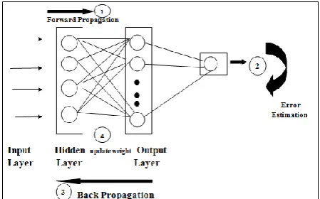
layers which are interconnected with each other as shown in Figure 1. Networks without cycles (feedback loops) and used when you input something at the input layer and it travels from input to hidden and from hidden to output layer are called FNNs networks (or perceptron) [26]. As shown in Figure 1, neurons implemented some computing operations over several inputs X = (x1; x2; · · · ; xm) and have one output
calculated through the activation function . In addition, neuron has a weight vector W = (wk1; wk2; ·· · ; wkn),
and a threshold or bias b. The full process of a neuron may be summarized as in (1) [27] [28].
(1)
where V, X, W and b represent output, input, weights and bias, respectively (·) denotes an activation function called sigmoid function as seen in (2) [27].
[image:2.595.317.542.169.309.2]
(2)
Fig.1. Topology of neural network
Second, Back Propagation Neural Network(BP-NN) algorithm. This algorithm could be divided into four main steps as shown in Figure 2: feed-forward computation, back propagation to the output layer and hidden layer, and weight updates. After choosing the weights of the network randomly, the BP algorithm is used to compute the necessary corrections. The algorithm is stopped when the value of the error function has become sufficiently small [29]. We proposed feed forward-back propagation (NN). Thus, we implement feed forward computation as presented previously in (1) and (2). Moreover, there are many training algorithms: Levenberg-Marquardt (trainlm), Bayesian-Regularization (trainbr), Resilient Back propagation (trainrp), and Scaled Conjugate Gradient (trainscg). We should select proper training algorithm that could reduce the training time effectively in least possible time to provide optimum results [30] [31]. Thus, we use training algorithm Scaled Conjugate Gradient (trainscg) to provide faster training with excellent test efficiency. "trainscg" appear to execute fine for networks with a large number of weights. Moreover, "trainscg" updates the weights and biases along the steepest descent direction but is usually associated with poor convergence rate as compared to the Conjugate Gradient Descent algorithms, which generally result in faster convergence [32]. In the Conjugate Gradient Descent algorithms, a search is made along the conjugate gradient direction to determine the step size that minimizes the performance function along that line. This time-consuming line search is required during all the iterations of the weight update. However, the Scaled Conjugate Gradient Descent algorithm does not require the computationally expensive line search and at the same time has the advantage of the Conjugate Gradient Descent
algorithms [33]. Also, we can calculate the mean of the sum square error(MSE) in (3):
(3)
where w is weight vector, tik is the desired output values and
oik is the actual output values for the ith training pattern and
the kth output neuron, and I is the total number of training
patterns [34].
Fig.2. BP multilayer NN with one hidden layer
2.2
Deep Neural Networks (DNN)
We presented softmax function as a DNN to improve the model of recognize human activities. Softmax layer function is used mainly in neural network in case of normalizing exponential when there are multiclass in order to describe and calculate to which category some input belongs according to the highest probability as (4). The purpose of the softmax classification layer is simply to transform all the DNN activations in the final output layer to a series of values that can be interpreted as probabilities. So, the softmax function is applied onto the DNN outputs without an activation function or bias [35]:
(4)
where are the conditional probabilities in terms of the likelihood of event x occurring given that and Cj ,respectively. , are the probabilities of
observing respectively independently of each other. From the previous equation (5), the quantities are defined by (5):
(5)
where the normalized exponential is also known as the softmax function, as it represents a smoothed version of the ‘max’ function because, if ak aj all j k, then p(Ck|x) 1, and p(Cj|x) 0 [35]. Moreover is known as normalized exponential or softmax function, in which case the posterior probability is governed by a generalized linear model. For the case of k > 2 classes. Thus, the result of softmax function will always be a positive value, smaller than 1, and sum up to 1. The activation of the softmax function is a generalization of the logistic function that "squashes" a K-dimensional vector x of the arbitrary real values to a K-dimensional vector f(xi) of
real values in the range [0, 1] that add up to 1. The function is given in (6) [35]:
(6)
3.
THE PROPOSED METHOD
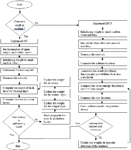
[image:2.595.56.281.252.418.2]one is how to form raw dataset to serve our experiments' needs, it splits the dataset to three forms (i.e. small, medium, and large). The second phase is to implement NN and DNN on three forms of dataset. The third phase is to obtain the results of training set and analyze the performance. The fourth phase is to implement NN and DNN on test sets taking into account the performance of the previous training models. Figure 3 has presented the proposed methods of NN and DNN. We detailed how to train NN and DNN as follows.
Fig.3. The proposed method to implement NN and DNN in different forms of dataset
3.1 NN implementation
We propose a multi-layer NN for HAR which consists of three main layers: input, hidden, and output layers. The input layer has N neurons, which indicates to the readings of the five sensor units. According to NN: two or three hidden layers are used in different number of neurons. Besides, the output layer has c neurons according to the number of activities. In each input and hidden layer there is an additional neuron with a bias value of 1. Add to that, we initialize weight to small random values. For each input feature vector, the target output is 1 for the class that the vector belongs to, and 0 for all other output neurons. The sigmoid function used as the activation function. The output layer consists of neurons that gives constant values between 0 and 1. We performed NN using back-propagation training algorithm by offering a set of training patterns to NN. The aim is to minimize the average of the sum squared errors over all training vectors. When the entire set finished their training completely, in terms of finishing first epoch. The difference between the desired and actual outputs values is calculated at the end of each iteration which is called the error. The average of these errors is computed at the end of each epoch. The training process is stopped when a certain reached goal on the average error is achieved or if the specified maximum number of epochs is exceeded, whichever occurs earlier.
3.2 DNN implementation
We suggested to replace sigmoid logistic function by the softmax function φ. Softmax function computes the probability that this training sample x(i) belongs to
class j given the weight and network input f(xi). So, we
compute the probability p(y = j | x(i); wj) for each class label in j = 1, ..., k. Starting by defining classes and compute the network input. After that we encode the class labels into format called one-hot encoding. Then, we compute the softmax activation. Next, define a cost function which refers to the average of all cross-entropies over the training samples. After that we learn our softmax model via gradient descent for each class. Finally, after using this cost gradient, we iteratively update the weight of training sample until we reach a specified number of epochs (passes over the training set) or reach the desired cost threshold.
4.
EXPERIMENTS AND RESULTS
This section is divided into 6 subsections. First, we describe the DSA dataset and the forms which we have comprised. Second, we introduced the performance measures which we adopted to compare between NN and DNN. Third, we describe the parameters settings for NN and DNN. The last three subsections include the three experiments: on small, medium, and large datasets and their results.
4.1 Dataset Description
The Daily and Sports Activities data set (DSA) is a real dataset in education which collects data at the sports hall in the electrical and electronics engineering building, at Bilkent University. It contains 19 activities. These activities are performed by 8 subjects (4 female, 4 males between the ages 20 and 30). Total signal duration is 5 minutes for each activity of each subject. There are 5 units which is putted on five various position on body like: torso (T), right arm (RA), left arm (LA), right leg (RL), left leg (LL). The data were collected from 3triaxial accelerometer (x,y,z), gyroscope (x,y,z) and magnetometer (x,y,z). In addition, it is clearly seen in Table 1 the total description of DSA dataset that has 5 units ×9 sensors = 45 columns and 5 seconds ×25 Hz = 125 rows [33].
DSA dataset matches our needs according to the main purpose to perform classification algorithms in order to recognize and infer activities. Also, the number of features and users are sufficient. The raw data are acquired accurately using sensors to avoid incomplete data and feeling uncomfortable if cameras have been used. Thus, we have formed the training data into 3sets: small, medium, and large in Table 2. First, the small dataset has been composed of selecting one row of each segment. So, we have (1×60×8=480 row per each activity) and we have (480×19=9120 row) and (5units×9 readings =45column). Second, the medium dataset has (4×60×8=1920 row per each activity) and we have (1920×19=36480 row). Third, the large dataset has (100×60×8=48000 row per each activity) and we have (48000×10=480000 row).
Table 1. Description of DSA data set
Elements of dataset Value
Number of subjects 8
Number of activities 19 Number of sensor location(units) 5 Number of sensor readings 9
Number of segments 60
Total number of rows 125 row per segment Total number of columns 9 × 5 = 45 columns Total number of rows per each
activity regarding to 8 subjects
125×60×8 = 60,000 rows
[image:3.595.55.278.171.426.2]Table 2.The forms of small, medium, and large datasets
Small Medium Large
Instances per segment 1 row 4rows 100rows
Total Instances per each activity to 8 subjects
1×60×8= 480
4×60×8=19 20
100×60×8 =48000
Total Instances 480×19=
9120
1920×19=3 6480
48000×10 =480000
Train Instances 6080 24320 32000
Test Instances 3040 12160 16000
4.2 Performance Measures
We adopted MSE, logistic regression, time as performance measures of NN. Moreover, we depend on ROC curve as performance evidence of DNN.
4.3 Parameters Settings
We describe parameters of NN: Maximum number of epochs to train, Performance goal, Maximum validation failures, Minimum performance gradient, Epochs between displays (NaN for no displays), Learning rule, Number of hidden layers, Number of neurons on each hidden layer, Activation function, and Performance function evaluation on Table3.
Table 3. The parameters set up of NN
Name Value
Max number of epochs to train 1000
Performance goal 0.01
Maximum validation failures 1000
Minimum performance gradient 1e-10 Epochs between displays (NaN for no displays) 10
Learning rule 0.3
Training algorithm trainscg
Number of hidden layers 3
Number of neurons on each hidden layer [33-8-5]
Activation function Sigmoid
Performance function evaluation MSE
Table 4has illustrated parameters set up of DNN: Number of max Epochs, Training algorithm, Performance function evaluation, and Activation function.
Table 4. The parameters set up of DNN
Parameters Value
Number of maxEpochs 500
Training algorithm trainscg
Performance function evaluation cross entropy, MSE Activation function Softmax function
4.4 Experiment 1: using the small dataset
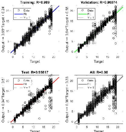
[image:4.595.321.535.82.528.2]The small dataset contains of (9120 × 45) feature vectors. We designed NN consists of three layers: input layer consists of 45 feature vectors, hidden layers contain 3 layers with different number of neurons (33-8-5), and 19 neurons on the output layer which specifies the activity label. Figure 4 shows the regression plot of NN on small dataset. Moreover, Figure 5 have presented the ROC curve for DNN on small dataset. Table 5 has illustrated the results that we obtained from the experiment on small dataset. It is clearly that we normalize all set up parameters as seen in Table 3 and Table 4 between NN and DNN in terms to demonstrate the difference only between NN and DNN.
Fig.4. The regression plot of NN (3hidden layers [33-8-5]) using "trainscg" on small dataset
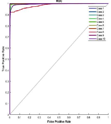
Fig.5. The ROC curve of DNN for test set on small dataset
We observe that ROC curve has medium accuracy according to test set because all of activities curves not collected in the upper left corner.
[image:4.595.50.285.88.175.2]Table 5. Results of NN and DNN on small dataset
Training algorithm NN DNN
Time 00:00:28 00:00:10
Number of Epochs 1000 500
Performance in train 1.1880 0.0140 Performance in test --- 0.1121 Accuracy for training 0.989 0.922697368 Accuracy for test 0.95817 0.679315789
4.5 Experiment 2: using the medium dataset
[image:5.595.317.540.124.206.2]This medium dataset consists of )36480 × 45) feature vectors. We used the same design of NN mentioned in Section 4.1 and the same experimental parameters in Table 3 and Table 4 for both NN and DNN. Therefore, Figure 6 has described the regression plot of NN on medium dataset. Add to that Roc curve for DNN on medium dataset has introduced in Figure 7.
Fig.6 The regression plot of NN (3hidden layers [33-8-5]) using "trainscg" on medium dataset
Fig.7. The ROC curve of DNN for test set on medium dataset
[image:5.595.63.276.271.497.2]We observe that ROC curve has medium accuracy according to test set because all of activities curves not collected in the upper left corner.
Table 6. Results of NN and DNN on medium dataset
Training algorithm NN DNN
Time 00:11:03 00:00:40
Number of Epochs 1000 500
Performance in train 0.6369 0.0152 Performance in test --- 0.1207 Accuracy for training 0.99196 0.91739 Accuracy for test 0.98343 0.67434
Table 6 has illustrated the results that we obtained from the experiment on medium dataset. Taking into account the results of NN achieved (0.99196) accuracy for training higher than DNN which achieved (0.91739) on medium dataset. Moreover, NN achieved (0.98343) accuracy for test higher than DNN which achieved (0.67434) on medium dataset. In contrast, DNN took approximately only 40 seconds lower than NN which took11 minutes and 3 seconds. Besides that, the number of epochs in DNN has decreased to a half comparing with NN and that indicates the high power of DNN. Besides that, MSE rate has (0.0152) in train and (0.1207) in test according to DNN which is lower than NN because it achieved (0.6369). That refers the performance of DNN.
4.6 Experiment 3: using the large dataset
This large dataset consists of (480000 × 45) feature vectors. Therefore, we divided sample into 66% (320000) for training and 33% (160000) for testing. We used the same design of NN mentioned in Section 4.1 and the same experimental parameters in Table 3 and Table 4 for both NN and DNN. According to results NN failed to train this large dataset. It stopped training at epoch 60 without complete training and that refers to NN not capable to train large datasets. In contrast, DNN as seen in Figure 8 ROC curve has achieved high accuracy to test set because all of activities curves are collected in the upper left corner.
[image:5.595.322.537.502.742.2] [image:5.595.64.272.521.756.2]Table 7. Results of NN and DNN on large dataset
Training algorithm NN DNN
Time fail 00:04:05
Number of Epochs fail 500
Performance in train fail 5.40e-04 Performance in test fail 0.0169 Accuracy for training fail 0.99900 Accuracy for test fail 0.97741
Table 7 has introduced the results that we obtained from the experiment on large dataset. Taking into account the results of NN which failed to train large dataset. While DNN achieved (0.9990) accuracy for training and (0.9774) for test. Moreover, DNN took only 4 minutes and 5 seconds to train large dataset. In addition, we have concluded that NN using "trainscg" achieved high training and testing regression on small and medium dataset in terms of NN is the best choice in dealing with small and medium dataset size regarding to performance and computational cost. In contrast, DNN is the best choice for large dataset.
5. CONCLUSION
This paper had presented as a guideline to design systems based on context-aware used wearable inertial sensors in order to serve HAR domain. The main purpose is to recognize human activities using neural classifiers: NN and DNN and applied them on small, medium, and large datasets to analyze the performance of NN and DNN. We discuss the results in terms of correct differentiation rates, confusion matrix, and computational cost. The results discovered that NN is the best choice for small and medium datasets. While DNN is the best choice for large datasets. According to NN, small dataset achieved (0.989) for training regression and (0.95817) for test regression using (3) hidden layers. Besides, medium dataset achieved (0.99196) for training regression and (0.98343) for testing regression. In addition, the results showed that DNN reduce the computational cost than NN, increase the performance of network, and achieved high overall successful differentiation rate in training (0.9990) and test (0.97742) on large dataset than on medium dataset (67.81%). or on small dataset (67.63%).
In future work, we intend to improve the DNN approach for other domains of HAR like: gestures, events, group actions, human to human interactions, and human or object interactions. Also, we intend to build an interactive application based on HAR to provide a recommendation or notifications to enable humans for adapting future events to live better lives.
6. REFERENCES
[1] Zhang, M., & Sawchuk, A. A. (2012, September). USC-HAD: a daily activity dataset for ubiquitous activity recognition using wearable sensors. In Proceedings of the 2012 ACM Conference on Ubiquitous Computing (pp. 1036-1043). ACM.
[2] Manzi, A., Dario, P., & Cavallo, F. (2017). A Human Activity Recognition System Based on Dynamic Clustering of Skeleton Data. Sensors, 17(5), 1100. [3] Attal, F., Mohammed, S., Dedabrishvili, M.,
Chamroukhi, F., ukhellou, L., & Amirat, Y. (2015). Physical human activity recognition using wearable sensors. Sensors, 15(12), 31314-31338.
[4] Thomaz, E., Bedri, A., Prioleau, T., Essa, I., &Abowd, G. D. (2017, June). Exploring Symmetric and
Asymmetric Bimanual Eating Detection with Inertial Sensors on the Wrist. In Proceedings of the 1st Workshop on Digital Biomarkers (pp. 21-26). ACM. [5] Ordónez, F. J., de Toledo, P., & Sanchis, A. (2013).
Activity recognition using hybrid generative/ discriminative models on home environments using binary sensors. Sensors, 13(5), 5460-5477.
[6] Barshan, B., &Yüksek, M. C. (2013). Recognizing daily and sports activities in two open source machine learning environments using body-worn sensor units. The Computer Journal, 57(11), 1649-1667.
[7] Lee, K., & Kwan, M. P. (2018). Physical activity classification in free-living conditions using smartphone accelerometer data and exploration of predicted results. Computers, Environment and Urban Systems, 67, 124-131.
[8] Sasaki, J. E., Hickey, A., Staudenmayer, J., John, D., Kent, J. A., & Freedson, P. S. (2016). Performance of activity classification algorithms in free-living older adults. Medicine and science in sports and exercise, 48(5), 941.
[9] Kaghyan, S., &Sarukhanyan, H. (2012). Activity recognition using K-nearest neighbor algorithm on smartphone with tri-axial accelerometer. International Journal of Informatics Models and Analysis (IJIMA), ITHEA International Scientific Society, Bulgaria, 1, 146-156.
[10]Rodrigues, L. M., &Mestria, M. (2016, August). Classification methods based on bayes and neural networks for human activity recognition. In Natural Computation, Fuzzy Systems and Knowledge Discovery (ICNC-FSKD), 2016 12th International Conference on (pp. 1141-1146). IEEE.
[11]Liu, L., Wang, S., Su, G., Huang, Z. G., & Liu, M. (2017). Towards complex activity recognition using a Bayesian network-based probabilistic generative framework. Pattern Recognition, 68, 295-309.
[12]Fan, L., Wang, Z., & Wang, H. (2013, December). Human activity recognition model based on Decision tree. In Advanced Cloud and Big Data (CBD), 2013 International Conference on (pp. 64-68). IEEE.
[13]Sarkar, A. J., Lee, Y. K., & Lee, S. (2010). A smoothed naive bayes-based classifier for activity recognition. IETE Technical Review, 27(2), 107-119.
[14]Namdari, H., Tahami, E., & Far, F. H. (2017). A comparison between the non-parametric and fuzzy logic-based classification in recognition of human daily activities. Biomedical Engineering: Applications, Basis and Communications, 29(01), 1750003.
[15]Lee, Y. S., & Cho, S. B. (2016). Layered hidden Markov models to recognize activity with built-in sensors on Android smartphone. Pattern Analysis and Applications, 19(4), 1181-1193.
a real-time human movement classifier using a triaxial accelerometer for ambulatory monitoring. IEEE transactions on information technology in biomedicine, 10(1), 156-167.
[18]Carós, J. S., Chetelat, O., Celka, P., Dasen, S., & CmÃral, J. (2005). Very low complexity algorithm for ambulatory activity classification. In 3rd European Medical and Biological Conference EMBEC (pp. 16-20). [19]Hammerla, N. Y., Halloran, S., &Ploetz, T. (2016). Deep, convolutional, and recurrent models for human activity recognition using wearables. arXiv preprint arXiv:1604.08880.
[20]Almaslukh, B., AlMuhtadi, J., & Artoli, A. (2017). An Effective Deep Autoencoder Approach for Online Smartphone-Based Human Activity Recognition. International Journal of Computer Science and Network Security (IJCSNS), 17(4), 160.
[21]Schmidhuber, J. (2015). Deep learning in neural networks: An overview. Neural networks, 61, 85-117. [22]Sze, V., Chen, Y. H., Yang, T. J., &Emer, J. (2017).
Efficient processing of deep neural networks: A tutorial and survey. arXiv preprint arXiv:1703.09039.
[23]Vepakomma, P., De, D., Das, S. K., &Bhansali, S. (2015, June). A-Wristocracy: Deep learning on wrist-worn sensing for recognition of user complex activities. In Wearable and Implantable Body Sensor Networks (BSN), 2015 IEEE 12th International Conference on (pp. 1-6). IEEE.
[24]Zhang, L., Wu, X., & Luo, D. (2015, December). Recognizing Human Activities from Raw Accelerometer Data Using Deep Neural Networks. In Machine Learning and Applications (ICMLA), 2015 IEEE 14th International Conference on (pp. 865-870). IEEE. [25]Lee, S. M., Yoon, S. M., & Cho, H. (2017, February).
Human activity recognition from accelerometer data using Convolutional Neural Network. In Big Data and Smart Computing (BigComp), 2017 IEEE International Conference on (pp. 131-134). IEEE.
[26]Shalev-Shwartz, S., & Ben-David, S. (2014).
Understanding machine learning: From theory to algorithms. Cambridge University press.
[27]Nogueira, K., Penatti, O. A., & dos Santos, J. A. (2017). Towards better exploiting convolutional neural networks for remote sensing scene classification. Pattern Recognition, 61, 539-556.
[28]Castrounis, A. (2016). Artificial Intelligence, Deep Learning, and Neural Networks, Explained. Available at:
https://www.kdnuggets.com/2016/10/artificial- intelligence-deep-learning-neural-networks-explained.html (last access: 5/12/2017).
[29]Rojas, R. (2013). Neural networks: a systematic introduction. Springer Science & Business Media. [30]Singh, A., Saxena, P., & Lalwani, S. (2013). A Study of
Various Training Algorithms on Neural Network for Angle based Triangular Problem. International Journal of Computer Applications, 71(13).
[31]Sahlol, A. T., Ewees, A. A., Hemdan, A. M., & Hassanien, A. E. (2016). Training feedforward neural networks using Sine-Cosine algorithm to improve the prediction of liver enzymes on fish farmed on nano-selenite. In Computer Engineering Conference (ICENCO), 2016 12th International (pp. 35-40). IEEE. [32]Tiwari, S., Naresh, R., & Jha, R. (2013). Comparative
study of backpropagation algorithms in neural network based identification of power system. International Journal of Computer Science & Information Technology, 5(4), 93.
[33]Møller, M. F. (1993). A scaled conjugate gradient algorithm for fast supervised learning. Neural networks, 6(4), 525-533.
[34]Altun, K., Barshan, B., & Tunçel, O. (2010). Comparative study on classifying human activities with miniature inertial and magnetic sensors. Pattern Recognition, 43(10), 3605-3620, available at: https://archive.ics.uci.edu/ml/datasets/Daily+and+Sports +Activities.