Abstract— Pharmacokinetic models, using recursive finite difference equations (RFDEs), can be derived directly from traditional exponential models. This method has been successfully applied to propofol infusion data. Furthermore, this technique yields identical accuracy, on a subject-specific basis, as the exponential model from which each RFDE model was derived. Specifically, these infusion models are based upon an inhomogeneous RFDE: P(k+3) = A·P(k+2) + B·P(k+1) + C·P(k) + R, where A, B, C, and R are non-zero constants and P represents plasma propofol levels for each kth unit of time. When applied to propofol infusions, RFDE modeling has advantages, over traditional exponential models, in that fewer coefficients are needed and patient-to-patient variation of these coefficients is reduced. However, initial conditions for RFDEs have to be specified. These characteristics, of RFDE modeling of propofol infusions, are similar to those for RFDE modeling of propofol boluses. Based on these findings, as well as those of our prior study, RFDE pharmacokinetic modeling can be applied to both infusion and bolus data of propofol. Further research, on the applications of RFDEs in pharmacokinetics, appears warranted.
Index Terms—pharmacokinetic models, propofol, recursive finite difference equations.
I. INTRODUCTION
Our previous research has shown that recursive finite difference equations (RFDEs) can be derived directly from traditional exponential pharmacokinetic models. Specifically, this modeling scheme was applied to a single bolus of propofol [1]. Thus, the RFDE model, based on a propofol bolus, was shown to have identical accuracy as the three-compartment exponential model from which it was derived.
Furthermore, each bolus RFDE model was derived using the form:
P(k+3) = AP(k+2) + BP(k+1) + CP(k), k = 1, 2, 3… (1) Glen Atlas is with the Department of Anesthesiology, University of Medicine and Dentistry of New Jersey, Newark, NJ and the Department of Chemistry, Chemical Biology and Biomedical Engineering, Stevens Institute of Technology, Hoboken, NJ, phone: (973) 972-5006 fax: (973) 972-4172, email: [email protected]
Sunil Dhar is with the Department of Mathematical Sciences, New Jersey Institute of Technology, Newark, NJ, email: [email protected]
Note that A, B, and C are dimensionless constant coefficients. In addition, these coefficients were shown to have decreased patient-to-patient variability when compared to those of the exponential model from which they were derived [1].
In modeling a propofol infusion, it is necessary to modify the above RFDE by adding a constant R:
P(k+3) = AP(k+2) + BP(k+1) + CP(k) + R, k = 1, 2, 3… (2) Note that R has the same “concentration” dimensions as each value of P. With R
0, (2) is known as an inhomogeneous RFDE whereas (1) is a homogeneous RFDE.Our initial study examined the pharmacokinetic properties of a propofol bolus using RFDEs [1]. This present study uses similar recursive mathematics to model the pharmacokinetic properties of a propofol infusion.
Propofol is an ultra-short acting sedative hypnotic. It should be recognized that propofol is frequently given, as a bolus, for the induction of general anesthesia. Propofol infusions can be used as an adjunct for the maintenance of general anesthesia and are also useful in providing continuous sedation.
Thus, the purpose of this study was to assess the utility of RFDE modeling for infusion-based pharmacokinetics. This study also shows how these equations can be derived directly from existing exponential infusion models. In this as well as our prior study, these are referred to as “parent” exponential models. Figure 1 illustrates the recursive nature of the pharmacokinetics of an infusion. As a drug is infused into the venous circulation, metabolism, redistribution, and excretion are occurring simultaneously. Subsequently, the remaining drug then returns, from the arterial side of the circulatory system, into the venous side. This occurs as the continuous infusion is maintained.
II. AN OVERVIEW OF INHOMOGENEOUS RFDE MODELS
FOR INFUSION-BASED PHARMACOKINETICS
In modeling infusion-based pharmacokinetics, with recursive finite difference equations (RFDEs), it is assumed that a steady-state “plateau” of a pharmaceutical blood level is eventually reached and sustained. Thus, the net rate of metabolism, elimination, and redistribution is not exceeded by the infusion.
Development of a Recursive Finite Difference
Pharmacokinetic Model from an Exponential
Model: Application to a Propofol Infusion
Figure 1: Conceptual diagram illustrating the recursive nature of pharmacokinetics with a constant infusion. Arterial propofol blood levels are metabolized, excreted, and redistributed. After passing through the heart, the venous drug concentrations become the subsequent arterial drug concentrations. Ultimately, the remaining propofol is again passed, to the venous system, with continuously-infused additional medication. Thus, RFDEs may be useful for modeling this recursive pharmacologic phenomena.
With this in mind, a straightforward single-compartment model can be examined. Using an RFDE this would be:
P(k+1) = C1P(k) + C2, k = 1, 2, 3… (3) Note that each value of P(k+1) is a function of its prior value P(k). Furthermore, an initial condition has to be specified. In the above formula, this would be a known value representing P(1).Using the above assumptions, the constants C1 and C2 must have the following properties: 0 < C1 < 1 and C2 > 0. A solution of (3) can be shown as [2], [3]:
*,
)
*
1 1) -( 1 )(
C
P
P
P
P
kk
(
k = 1, 2, 3… (4) Where P1 represents the initial serum level of medication and P* = C2/(1 - C1). The reader should note that (4) represents the general solution of (3). In addition, the values determined from (4) do not need to be determined from prior values. Furthermore, the steady state plateau level that is ultimately reached is P* [3].These RFDEs are referred to as inhomogeneous as C2 is non-zero. The use of homogeneous RFDEs has been shown to be applicable in the modeling of propofol bolus data [1].
Furthermore, solutions to inhomogeneous RFDEs consist of the sum of the solution to the homogeneous equation super positioned, or added, to that of the particular solution. Thus, in the above case, the homogeneous solution is:
), ( 1 ) 1 -( 1 )
( C P
Phk k
k = 1, 2, 3…
(5)
Whereas the particular solution is:
), -1 ( * 1( -1) )
(
k p
k P C
P
k = 1, 2, 3…
(6)
The sum of the homogeneous solution, (5), and the particular solution, equation (6), yields the general solution to the inhomogeneous RFDE, as shown in (4):
, ) ( ) 1 ( ) ( * * 1 ) 1 -( 1 ) 1 -( 1 * 1 ) 1 -( 1 ) ( ) ( ) ( P P P C C P P C P P P k k k p k h k k
k = 1, 2, 3… (7)
Appendix A and Appendix B together demonstrate how a three compartment RFDE model is developed using the sum of its homogeneous and particular solutions.
III.NOMENCLATURE
Note that P(k+3) refers to the values generated from the inhomogeneous RFDE which is the sum of the homogeneous and particular solutions:
P(k+3) = AP(k+2) + BP(k+1) + CP(k) + R, k = 1, 2, 3...
(8) Whereas P(k) is the general solution to (8):
P(k) = h - k + kk) . (9) Also, note that Q(k) refers to the solution obtained from the traditional three-compartment exponential model:
Q(k) = h - (ae-bk + ce-dk + fe-gk) . (10) It should be noted that P(k+3) and P(k) and Q(k) are numerically equivalent. The terminology: k = 1, 2, 3... denotes that those values, obtained from an RFDE, must be calculated sequentially. This sequential process is unnecessary when using the general solution.
As will be subsequently shown, the RFDE model (8) is derived directly from its “parent” exponential model (10).
IV. DERIVING EACH RFDE MODEL FROM ITS RESPECTIVE PARENT EXPONENTIAL MODEL
A traditional three-compartment exponential model, for a continuous infusion, is based on the following equation:
Q(k) = h - (ae -bk
+ ce-dk + fe-gk) . (11) Equating (11) to the homogeneous solution of the finite difference model (9) with h = 0 yields:
k + kk) = (ae-bk + ce-dk + fe-gk ) . (12)
Note that the homogeneous solution requires that h = 0. Equation (12) is then valid under the following conditions:
= a, c, and = f
(13)
Arterial
Venous
Metabolism Redistribution Excretion Heart
[image:2.595.44.283.46.135.2]and
e-b, = e-d, = e-g
.
(14) Substituting the above relations, into the RFDE model from Appendix A, yields:P(k+3) = AP(k+2) + BP(k+1) + CP(k) + R, k = 1, 2, 3... (15) where:
A = ( + + ) = (e-b + e-g + e-d) (16) B = - ( + + ) = - (e-b•e-g + e-b•e-d + e-d•e-g) =
- (e-(b+g) + e-(b+d) + e-(d+g)) (17) C =e-b•e-d•e-g) = e-(b+d+g) (18) and R is the particular solution with h
(See: Appendix B):R = h•[1 - (A + B + C)] . (19)
Note that the solution to (15) represents the superposition, or summation, of the homogeneous and particular solutions (See: Appendix A and Appendix B).
The constant coefficients: A, B, and C, as well as the inhomogeneous constant R, of each RFDE model, are derived directly from those of their respective parent exponential models. Therefore, each RFDE model will have the same accuracy as the “curve-fitted” parent exponential model from which it was derived.
In this particular application, each RFDE was based on three dimensionless constant coefficients A, B, and C and a constant R. Whereas each exponential model, as well as the general solution of each RFDE, required six coefficients and a constant. Thus, the RFDE model is a more “compact” representation.
However, it is necessary to determine the initial conditions: P1, P2, and P3, for each RFDE. These can be obtained from either their general solution or their respective parent exponential model. With these initial values, each RFDE can then determine subsequent subject-specific propofol serum levels for the entire infusion.
A numerical example of this process is illustrated in Appendix C.
V. METHODS:DATA ACQUISITION AND ANALYSIS
Propofol serum levels for this study were obtained from prior research and supplied to the authors directly from Astra-Zeneca pharmaceuticals. Volunteers, in the initial IRB-approved study, age 19 through 65, who had received informed consent, had been given an intravenous bolus of propofol of 2 mg/kg. Patients over 65 had received boluses
of 1 mg/kg. Arterial serum propofol levels were then measured sequentially at 1, 2, 4, 8, 16, 30 and 60 minutes [4]. Analysis of this bolus data was the basis of our prior study [1].
One hour following each bolus, a propofol infusion was then started. Patients were assigned to infusion rates of 25, 50, 100, or 200 g/kg/min. Each infusion rate was assigned two patients whose ages were < 65 and two patients whose ages were > 65.
Samples for analysis were collected, from each patient, via a radial arterial catheter. Values analyzed, for this study, were those collected at 0, 2, 4, 8, 16, 30, and 60 minutes following the beginning of the infusion. These data are illustrated in Fig. 2.
It should be noted that the purpose of the original study was to assess the pharmacokinetics of propofol with, versus without, disodium edetate (EDTA). EDTA is an additive which inhibits microbial growth. The data, used in this study, were from those patients who had received formulations with EDTA.
This retrospective analysis, of existing data, was deemed exempt from requiring IRB approval at both authors’ institutions. Data from a total of the 16 original subjects met inclusion criteria for this present analysis.
Curve fitting was performed using MATHCAD (Mathsoft, Cambridge, MA). For each parent exponential model, this was based upon (See: Appendix A):
Q(k) = h - (ae -bk
+ ce-dk + fe-gk). (20) Specifically, a minimum error function, based upon the Levenberg-Marquardt algorithm, was used [8], [9]. Iterations were performed until the mean sum of the squared error (MSSE) was on the order of 10-1 or less:
. )}) e e e ( { ( 1
MSSE 2
1
gj n
j
dj bj
j h a c f
s n
(21) Where sj represents each measured propofol serum level
and n = 7 for each subject’s seven measurements. This process was repeated for each subject-specific parent exponential model.
Following the determination of the exponential coefficients, and the constant h, the coefficients A, B, C and the constant R, for each RFDE model, were then calculated using the method described in equations (11) through (19). (See: Deriving each RFDE model from its respective parent exponential model). The flowchart in Fig. 3 summarizes these processes.
Figure 3. This flowchart depicts how each RFDE model was derived from its respective parent exponential model.
VI. RESULTS
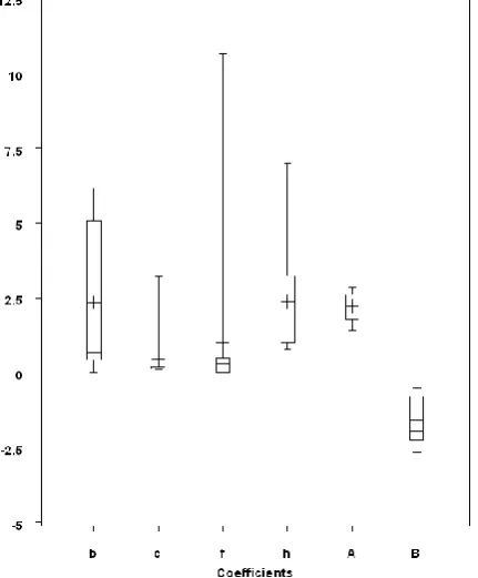
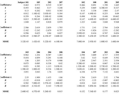
Table 1 documents the serum levels of propofol taken from the 16 patients during each infusion. After curve fitting to the parent exponential function, values for each of these coefficients are displayed in Table 2. Table 2 also lists the coefficients for the RFDE model for each patient. Furthermore, the mean sum of the squared error (MSSE) is also displayed. Note that the MSSE for each of the parent exponential models, and its RFDE model, are identical. This occurs as each RFDE model is derived directly from its respective subject-specific parent exponential model. Figures 4 and 5 illustrate both the parent and RFDE coefficients and constants graphically. Note that the RFDE coefficients A, B, C, and the constant R have less variability than those of their parent exponential models. This overall reduction in variability can be explained by use of the chain rule [5], [6]:
dA = b
b A d
+ d
d A
d
+
gg A d
(22)
dB = b b B d
+ d
d B
d
+ g
g B d
(23)
dC = b
b C
d
+
dd C
d
+
gg C
d
(24)
dR = b R
db + d R
dd + g R
dg + h R
dh . (25)
[image:5.595.46.270.65.254.2] [image:5.595.317.540.393.663.2] [image:5.595.70.287.550.709.2]The maximum change in coefficients A, B, C and R can then be expressed (See: Appendix D):
|dA| < {|db| + |dd| + |dg|}
(26)
|dB| < 2{|db| + |dd| + |dg|} (27) |dC| < {|db| + |dd| + |dg|}
(28) |dR| < m{|db| + |dd| + |dg|+ |dh|} where m = max(|h|, 1).
.
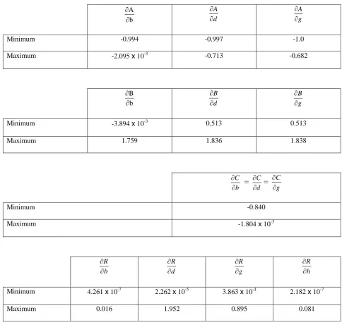
(29) Based on the infusion data, minimum and maximum values for the partial derivatives which determine dA, dB, dC, and dR can be obtained. These are summarized in Table 3.
The results of this study are similar to those of the authors’ prior examination of RFDE modeling of a propofol bolus.
Thus, the change in the coefficient A is less than the sum of the changes in coefficients b, d, and g. This also applies to the change in coefficient C. Whereas the change in coefficient B is less than twice the sum of the changes in b, d, and g.
Note that the change in coefficient R is less than a number which is proportional to the sum of the changes in b, d, g, and h.
Examination of Figures 4 and 5 shows that A, B, C, and R indeed have overall less variability as explained by equations (26) through (29).
Figure 4. A comparison of the coefficients and constants of the exponential and RFDE models. Note that C and R, of the RFDE models, have overall decreased variability. Also, coefficient a has the highest range, and inter-quartile range, as compared to d, g, C and R.
Subject-Specific Propofol Serum Levels
Curve Fit to Exponential
Derive Coefficients for RFDE
RFDE Model
Figure 5. A comparison of the coefficients and constants of the exponential and RFDE models. Coefficients b, f, and h have a higher range when compared to c, A and B. Furthermore, the inter-quartile ranges of b and h are higher than those of c, f, A and B.
VII. DISCUSSION
Recursive mathematics has successfully been applied in Fibonacci–related modeling, economics, and in social as well as the behavioral sciences. The results of this study, as well as the authors’ prior study, demonstrate that recursive mathematics can also be applied to pharmacologic models of both infusions and boluses of propofol. In addition, since each RFDE model is derived directly from its parent exponential model, there is no loss of accuracy.
Overall, RFDE modeling of infusions, as compared to traditional exponential modeling, has shown that fewer coefficients are needed. Furthermore, the patient-to-patient variability of these coefficients is reduced as compared to those of the exponential models. However, RFDE models require the establishment of initial conditions.
This modeling technique may be useful in computer-driven infusions utilizing servo or “feedback” to control serum propofol levels. Recently, plasma propofol levels have been shown to correlate with exhaled propofol concentrations [11]. Thus, the ability to do real-time control of propofol serum levels, with recursive modeling of pharmacokinetics, is possible.
Furthermore, systems of multiple RFDEs can also be solved simultaneously using such techniques as Z transforms and operator methods [2], [3], [4]. This may be applicable in examining drug-drug interactions.
VIII. CONCLUSIONS
The authors have demonstrated the applicability of RFDEs in three-compartment propofol infusion models. In addition, this modeling scheme is derived directly from traditional exponential models with no loss of accuracy. Our findings, in this paper, concur with those of our prior study of RFDE three-compartment propofol bolus models. Thus, RFDE models are more “compact” and their coefficients appear to have less patient-to-patient variability than exponential models. However, the specification, of initial conditions, is required for RFDE models.
Additional research would involve the analysis and applications of other medications and drug-drug interactions with recursive mathematics.
APPENDIX A: HOMOGENEOUS SOLUTION
It should be noted that a case-specific solution to an inhomogeneous finite difference equation consists of the sum of its homogeneous solution and its particular solution [2], [3], [4].
In this application, it is assumed that propofol serum levels are, initially, monotonically increasing. Thus, there is no oscillatory behavior noted as these initial levels consistently increase. Furthermore, after steadily increasing, a “plateau” level is ultimately reached and subsequently sustained.
The homogeneous solution of the RFDE is defined with the following form:
P(k+3) = AP(k+2) + BP(k+1) + CP(k), k = 1, 2, 3... (1A) Note that R is not included in the above equation. The solution for R represents the particular solution which is added to the homogeneous solution (See: Appendix B). In addition, the homogeneous solution, for equation (1A), has an identical form as that of three-compartment bolus-based models [1].
It should be noted that a solution to a first-order homogeneous finite difference equation:
, ) ( 1 ) 1 (k Czk
z k = 1, 2, 3... (2A) has a solution which has the form [2], [3]:
z( )k C C2 1k.
(3A)
allows for the representation of an increasing function which eventually reaches a plateau (See: Appendix B).
The solution to (1A) will have a form consisting of a superposition of solutions resembling (3A) [2], [3], [4]
.
P(k) = k + kk . (4A) The solution to (1A), using the form of (4A), requires the definition of a third-order characteristic equation [2], [3], [4]
.
(M -)(M -)(M -) = 0. (5A) Expanding (5A) and collecting terms yields:
3
M + (- - - )M2 + ( + + )M - = 0. (6A) Rearranging:
3
M = ( + + )M2 - ( + + )M+.
(7A) The solution will then take on the requisite form as:
P(k+3) = ( + + )P(k+2) - ( + + )P(k+1) + P(k), k = 1, 2, 3...
(8A) Therefore, by defining:
A = ( + + ) (9A) and B = - ( + + ) (10A) and C = . (11A) Equation (8A) will then take on the form of (1A): P(k+3) = AP(k+2) + BP(k+1) + CP(k), k = 1, 2, 3... (12A) Note that the inclusion of the inhomogeneous constant R allows for the modeling of a monotonically increasing function which eventually reaches a steady-state (See: Appendix B).
APPENDIX B: PARTICULAR SOLUTION The complete, or general solution, for an inhomogeneous RFDE, consists of the homogeneous solution (See: Appendix A) added to the particular solution [2], [3], [4]. In this case, the particular solution is a constant R:
P(k+3) = A·P(k+2) + B·P(k+1) + C·P(k) + R . (1B)
Rearranging yields:
P(k+3) - A·P(k+2) - B·P(k+1) - C·P(k) = R .
(2B) As a trial solution, it is reasonable to assume a time-invariant constant for each value of P(k+3), P(k+2) , P(k+1), and P(k). Substituting the constant h for P(k), which is identical over k from equation (9) and Q(k) from equation (10), yields:
h - A·h - B·h - C·h = R . (3B)
Simplifying equation (3B) yields an expression for R in terms of h:
R = h·[1 - (A + B + C)] . (4B)
This technique is known as the method of undetermined coefficients [2], [3], [4]. The value of h is chosen from examination of both equations (9) and (10) as k approaches infinity:
lim
k
P(k)=
lim
k
Q(k)=h
.
(5B)APPENDIX C: A NUMERICAL EXAMPLE The following is a numerical example which is based upon Table 1 subject 101. Using the exponential model from (10):
Q(k) = h - (ae-bk + ce-dk + fe-gk) . (1C) Based on non-linear curve fitting, coefficients for the above equation were found to be: a = 0.463, b = 0.493, c = 0.13, d = 0.012, f = 0.359, g = 0.013, and h = 1.048 . The general solution, P(k), is then determined from conditions (13) and (14):
P(k) = h - k + kk). (2C) Where
= a, c, and = f and e-b, = e-d, = e-g . (3C)
The coefficients, for the RFDE, P(k+3), can then be determined by first calculating A, B, and C from (9A), (10A), and (11A) respectively using (16-19):
A
= (
+
+
) = (e
-b+ e
-g+ e
-d)
= (e-0.493 + e-0.013 +e-0.012) =
2.586
(4C) B = -( + + ) = -(e-( b + g) + e-(b + d) + e-(d + g))
= -(e-0.506 + e-0.505 + e-0.025) = -2.181
(5C) C =e-b•e-d•e-g) = e-(b + d + g)
The homogeneous RFDE is then expressed as in (12A): P(k+3) = (2.586)P(k+2) - (2.181)P(k+1) + (0.596)P(k) ,
k = 1, 2, 3...
(7C) The inhomogeneous RFDE is:
P(k+3) = A·P(k+2) + B·P(k+1) + C·P(k) + R, k = 1, 2, 3...
(8C) The constant R is then determined using the method of undetermined coefficients (See: Appendix B):
R = h·[1 - (A + B + C)].
(9C) Note that R must be calculated with extreme accuracy as rounding errors can accumulate with recursive calculations:
R = 1.0484143·[1 – (2.5862913 – 2.1823666
+ 0.5960156)] = 6.24·10-5
.
(10C) Thus, the complete solution is the superposition, or sum, of equations (7C) and (10C):P(k+3) = (2.586)P(k+2) - (2.181)P(k+1) + (0.596)P(k) + 6.24·10-5, k = 1, 2, 3...
(11C) It should be noted that the initial conditions: P(1), P(2), and P(3) are determined from either (1C) or (2C). Thus, (1C), (2C) and (7C) yield numerically identical results for the entire time period.
The initial conditions, for this case, are: P1 = 0.096, P2 = 0.283, and P3 = 0.399 g/ml.
APPENDIX D
In order to assess the decrease in patient-to-patient variability, of the coefficients of the RFDE models, as compared to those of the exponential models from which they are derived, it is important to first note that coefficients b, d, and g are all numerically nonnegative and nonzero.
It should be noted that the changes in coefficients A, B, and C are identical, with respect to their derivation, for both the bolus and infusion RFDE models [1].
Therefore:
1 e
-0 -b and
0-e-d 1 and 0-e-g 1.
(1D) The variation in coefficient A can then be expressed using the chain rule [9]:
dA = b
b A d + d d A d + g g A d (2D)
It is assumed that db, dd, and dg are all ≥ 0. Realizing that: b
b A -e -
and d
d A -e - and g g A-e
-
. Equation (2D) can then be expressed as: dA = [-e-b]db + [-e-d]dd + [-e-g]dg
.
(3D) Under these circumstances, the triangle inequality will be such that the absolute value of the sum will be less than the sum of the absolute values [10]. This and (1D) therefore yield the following valid expression:
|dA| {|e-bdb| + |e-ddd| + |e-gdg|}
.
(4D) Therefore: |dA| < {|db| + |dd| + |dg|}. Similarly, the patient-to-patient variation, in coefficient B is:dB = b
b B d + d d B d + g g B d
(5D)
In this case:
b B
= e
-(b + g)+ e
-(b + d) andd B
= e
-(b + d)+ e
-(d + g) andg B
= e
-(b + g)+ e
-(d + g).
Equation (5D) can then be expressed as: dB = e-b{[e-d] + [e-g]}db + e-d{[e-b] + [e-g]}dd
+ e-g{[e-b] + [e-d]}dg. (6D) Again, use of the triangle inequality yields:
|
dB| {|e-b{[e-d] + [e-g]}db| + |e-d{[e-b] + [e-g]}dd| + |e-g{[e-b] + [e-d]}dg|}.(7D) Equation (7D) can then be expressed as:
|dB| 2{|e-bdb| + |e-ddd| + |e-gdg|}.
(8D) So that: |dB| < 2{|db| + |dd| + |dg|}.
Also,
dC = b
b C d + d d C d + g g C d (9D)
In this case:
b C = d C = g C
=-e-(b + d + g) so that:
Similarly,
|dC| {|e-(b + d + g)|•[|db| + |dd| + |dg|]}
.
(11D) Therefore: |dC| < {|db| + |dd| + |dg|}.Thus, the magnitude, of the patient-to-patient variation in coefficient A, will be less than the sum of: db, dd, and dg. This similarly applies to C.
Whereas the magnitude, observed in the patient-to-patient variation of coefficient B, will be less than twice the sum of: db, dd, and dg.
The patient-to-patient variation in the constant R can also be assessed. Recall that R is defined in terms of A, B, C, and h (See: Appendix B):
R = h·[1 - (A + B + C)]. (12D)
Substituting the definitions of coefficients A, B, and C from equations (16), (17), and (18) yields:
R = h·[1 - ({e-b + e-g + e-d}-{e-(b + g) + e-(b + d)
+ e-(d + g)} + {e-(b + d + g)})]. (13D) After differentiation and algebraic simplification, the following relationships can be stated:
] e 1 ][ e 1 [
e-b -g -d h b R (14D) ] e 1 ][ e 1 [
e-d -b -g h d R (15D) ] e 1 ][ e 1 [
e-g -b -d h
g
R
(16D) and, ] e 1 ][ e 1 ][ e 1
[ -b -g -d
h
R
. (17D)
The total change in R can also be expressed using the chain rule: dR = b R db + d R
dd + g R
dg + h R
dh (18D)
dR = he-b[1e-g][1e-d]db + he-d[1e-b][1e-g]dd + he-g[1e-b][1e-d]dg
+ [1e-b][1e-g][1e-d]dh . (19D) The following inequalities should be noted:
1 e
-0 -b and 0 -e-d 1 and 0 -e-g 1 (20D)
and
1 e -1
0 -b and
01-e-d 1 and
0 -e-g 1
(21D) Equation (19D) can then be expressed as an inequality:
|dR| < h{|db| + |dd| + |dg|} + |dh|.
(22D) Therefore, small changes in R are less than a value which is proportional to the sum of the small changes in b, d, g, and h. If m = max(|h|, 1) then:
|dR| < m{|db| + |dd| + |dg|+ |dh|}
.
(23D)REFERENCES
[1] G. Atlas & S. Dhar, Development of a Recursive Finite Difference Pharmacokinetic Model from an Exponential Model: Application to a Propofol Bolus, J. Pharm Sci, 95, 2006, 810-820.
[2] R. Mickens, DIFFERENCE EQUATIONS THEORY AND APPLICATIONS, 2nd Edition, New York, Van Nostrand Reinhold, 1990.
[3] S. Goldberg, INTRODUCTION TO DIFFERENCE EQUATIONS, New York, Dover Publications, 1986. [4] H. Levy & F. Lessman, FINITE DIFFERENCE EQUATIONS, New York, Dover Publications, 1992. [5] J.R. Sneyd, Recent Advances in Intravenous Anesthesia, British Journal of Anesthesia, 93(5), 2004, 725-736.
[6] T.W. Schnider, et al, The Influence of Method of Administration and Covariates on the Pharmacokinetics of Propofol in Adult Volunteers, Anesthesiology, 88(5), 1998, 1170-1182.
[7] K. Levenberg, A Method for the Solution of Certain Problems in Least Squares, Quart. Appl. Math 2, 1944, 164-168.
[8] D. Marquardt, An Algorithm for Least-Squares Estimation of Nonlinear Parameters, SIAM J. Appl. Math, 11, 1963, 431-441.
[9] C.H. Edwards & D.E. Penney, CALCULUS, New Jersey, Prentice-Hall, 2002.
[10] T. Apostol, MATHEMATICAL ANALYSIS, 2nd Edition, Boston, Addison-Wesley, 1974.
Table 1. Measured serum propofol levels, for each of the 16 subjects, at the specified times. Note that serum levels are in units of micrograms/ml.
Subject 101 105 202 207
infusion 25
g/kg/min
infusion 25
g/kg/min
infusion 25
g/kg/min
infusion 25
g/kg/min
Time0 0.1100 0.1120 0.2040 0.1910
2 0.3220 0.4470 0.5560 0.7020
4 0.6320 0.5960 0.4090 0.7930
8 0.5610 0.7440 0.6310 0.8550
16 0.6060 0.6390 0.7630 1.0100
30 0.7480 0.7630 0.7750 0.9580
60 0.8120 0.7850 0.7780 0.9680
102 108 201 205
infusion 50
g/kg/min
infusion 50
g/kg/min
infusion 50
g/kg/min
infusion 50
g/kg/min
Time0 0.1190 0.2500 0.1540 0.1160
2 0.7680 0.8620 0.5190 0.6220
4 0.8470 0.9470 0.9300 0.8500
8 1.0000 1.1600 1.1200 0.9430
16 1.2200 1.1600 1.3900 0.9210
30 1.2100 1.3000 1.4800 1.3900
60 1.2000 1.8200 1.7900 2.8200
103 106 204 208
infusion 100
g/kg/min
infusion 100
g/kg/min
infusion 100
g/kg/min
infusion 100
g/kg/min
Time0 0.2440 0.2010 0.0804 0.1410
2 0.8420 1.6600 1.1100 1.9000
4 1.8000 1.8200 1.4000 1.6400
8 1.8000 2.1000 1.6800 2.2100
16 2.4700 2.4500 1.9000 2.3600
30 2.9400 2.7100 1.6400 2.4600
60 2.9700 2.9100 1.7400 2.7700
104 107 203 206
infusion 200
g/kg/min
infusion 200
g/kg/min
infusion 200
g/kg/min
infusion 200
g/kg/min
Time0 0.1510 0.1830 0.1370 0.1310
2 3.5400 2.4600 2.7800 3.0800
4 3.6100 3.2600 4.9900 3.3100
8 4.4100 4.0000 5.6800 4.3400
16 4.5900 4.6200 5.7000 4.6500
30 3.5700 4.8300 7.4800 4.4100
[image:11.595.64.530.187.567.2]
Table 2. Note that a, b, c, d, f , and g are the coefficients for the parent exponential models and h represents its associated constant. Whereas A, B, and C are the coefficients for each RFDE model and R represents its associated constant. MSSE refers to the mean sum of the squared error which is identical for each RFDE and its parent exponential model.
Subject 101 105 202 207 102 108 201 205
Coefficient a 0.463 0.573 0.519 0.387 0.466 0.691 1.398 1.645
b 0.493 0.462 0.17 3.248 5.239 0.869 6.30E-03 0.327
c 0.13 0.202 0.011 0.303 0.14 3.338 1.064 -2.47
d 0.012 1.10E-02 3.03E-03 0.184 0.147 4.49E-03 0.253 0.09
f 0.359 0.264 3.10E-02 0.098 0.498 0.184 0.448 10.662
g 0.013 5.39E-05 1.60E-03 0.183 0.147 4.69E-03 6.02E-03 6.68E-03
h 1.048 1.147 0.818 0.979 1.223 4.464 3.048 9.948
Coefficient A 2.586 2.619 2.839 1.703 1.731 2.41 2.764 2.628
B -2.182 -2.242 -2.679 -0.757 -0.754 -1.826 -2.531 -2.282
C 0.596 0.623 0.84 0.027 3.95E-03 0.416 0.767 0.654
R 6.25E-05 2.58E-07 6.15E-07 2.60E-02 2.30E-02 5.43E-05 2.57E-05 1.60E-03
MSSE 3.32E-03 1.42E-03 5.22E-03 6.10E-04 7.80E-04 2.93E-03 1.80E-03 1.60E-04
103 106 204 208 104 107 203 206
Coefficient a 0.962 1.254 0.387 1.483 2.598 3.609 4.717 1.935
b 0.454 4.859 5.291 6.168 3.62 0.43 0.449 5.592
c 1.86 1.203 0.179 0.908 2.268 2.947 2.351 2.558
d 0.075 0.085 0.338 0.02 5.28E-03 0.016 0.067 0.218
f 0.021 0.385 1.113 5.03E-01 1.32E+00 2.20E-02 2.73E-03 1.70E-02
g 1.30E-02 1.80E-02 0.336 1.30E-01 3.83E-01 1.60E-02 5.50E-02 1.20E-02
h 3.051 3.043 1.76 3.035 6.338 6.779 7.132 4.641
Coefficient A 2.55 1.909 1.433 1.86 1.704 2.619 2.52 1.796
B -2.132 -0.918 -0.517 -0.865 -0.723 -2.25 -2.087 -0.802
C 0.582 7.00E-03 2.57E-03 1.80E-03 0.018 0.63 0.565 2.96E-03
R 1.04E-03 4.31E-03 0.143 7.19E-03 1.00E-02 5.85E-04 8.90E-03 1.10E-02
Table 3. Minimum and maximum values of the partial derivatives for equations (22-25). These explain the overall reduction, in patient-to-patient variability, seen in the coefficients of the RFDEs. This is in comparison to the coefficients of their respective parent exponential models. It should be noted that minimum refers to the smallest value whereas maximum refers to the greatest value.
b A
d A
g A
Minimum -0.994 -0.997 -1.0
Maximum -2.095 x 10⁻³ -0.713 -0.682
b B
d B
g B
Minimum -3.894 x 10⁻³ 0.513 0.513
Maximum 1.759 1.836 1.838
b C
=
d C
=
g C
Minimum -0.840
Maximum -1.804 x 10⁻³
b R
d R
g R
h R
Minimum 4.261 x 10⁻⁷ 2.262 x 10⁻⁵ 3.863 x 10⁻⁴ 2.182 x 10⁻⁷
Maximum 0.016 1.952 0.895 0.081
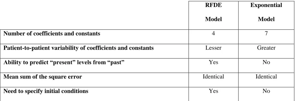
[image:12.595.54.539.194.655.2]Table 4. Comparison of the exponential and RFDE modeling of propofol infusions.
RFDE
Model
Exponential
Model
Number of coefficients and constants 4 7
Patient-to-patient variability of coefficients and constants Lesser Greater
Ability to predict “present” levels from “past” Yes No
Mean sum of the square error Identical Identical