Dynamical tuning of energy transfer efficiency on a graphene monolayer
Vasilios D. Karanikolas, Cristian A. Marocico, and A. Louise Bradley*
Semiconductor Photonics Group, School of Physics and CRANN, Trinity College Dublin, College Green 2, Dublin, Ireland (Received 15 November 2014; revised manuscript received 23 January 2015; published 16 March 2015) In this contribution we present a theoretical investigation of the energy transfer efficiency between quantum systems placed in proximity of a monolayer of conducting graphene. We calculate the spontaneous emission rate of a quantum system and the energy transfer rate between a donor-acceptor pair, and thus the energy transfer efficiency, using a Green’s tensor formalism. The direct interaction between the donor and acceptor dominates when they are close to each other, but is modified from its free-space behavior due to the presence of the graphene monolayer and its interaction with the donor and acceptor. We report on a very large influence of the graphene monolayer on the energy transfer efficiency due to both the F¨orster mechanism and the propagating graphene plasmon mode. In particular, the F¨orster radiusR0is modified from its free-space value of 20 nm and can reach values of 120 nm when close to a graphene monolayer. As the donor-acceptor separation is increased, their direct interaction is overshadowed by the interaction via the surface plasmon mode. Due to the large propagation length of the surface plasmon mode on graphene, an energy transfer efficiency as high as 50% can still be achieved for distances as large as 300 nm. The interaction via the surface plasmon mode is tunable via the doping of the graphene monolayer and the surface plasmon channel can also be switched off this way.
DOI:10.1103/PhysRevB.91.125422 PACS number(s): 33.80.−b
I. INTRODUCTION
For the last two decades the field of plasmonics has grown intensively. Confining light to subwavelength structures by exciting surface plasmon-polariton (SPP) modes has various applications in biosensing devices, light harvesting, optical nanoantennas, and quantum information processing. SPPs are collective oscillations of electrons and the electromagnetic field that are excited at the interface between a dielectric and a conductor and can propagate along that interface [1]. In plasmonics, noble metals are routinely used as the conducting medium. The main drawback of using noble metals in the applications mentioned above is their large ohmic losses [2].
Graphene constitutes an alternative to using noble metals for plasmonic applications [3–7]. It is a two-dimensional material possessing unique properties. This atomically thick monolayer has superior electronic and mechanical properties originating in part from its charge carriers of zero effective mass that can travel for microns without scattering at room temperatures [8].
An undoped graphene monolayer (GM) can absorbπ α0≈ 2.3% of the light incident upon it, whereα0is the fine structure constant [9]. Patterned GM nanostructures can give rise to 100% absorption at specific wavelengths, which can be tuned through the applied voltage [10–12].
Interactions between quantum emitters (QEs) and a GM have been investigated intensively over the last few years, es-pecially regarding the influence of the GM on the spontaneous emission (SE) rate of a QE placed near the GM [13–19]. It has been found that the SE rate can be enhanced by several orders of magnitude compared with its free space value, due to the excitation of graphene plasmon (GP) modes. Furthermore, confinement of the GP modes to one dimension (graphene ribbons) [12,17] and zero dimensions (graphene nanodisks) [11,17,20] can enhance the QE-GM interaction even more. In
the case of zero-dimensional confinement, the strong-coupling regime can be achieved between a QE and graphene nanodisks [17].
The presence of a second QE in the system will modify the emission properties of the system, giving rise to super-and subradiant states [21,22]. Furthermore, the confinement of the GP to one dimension (graphene ribbons) [23] or zero dimensions (graphene nanodisks) [20] further enhances the interaction rates. Although the SE of a QE in the presence of graphene nanostructures has been investigated thoroughly, the energy transfer (ET) rate between a pair of QEs in the presence of graphene nanostructures has garnered less attention. In particular, it is an open question whether or not it is possible to allow efficient interaction between a pair of QEs in the presence of a GM [24,25]. The authors of Ref. [24] have found an enhancement of the resonance ET rate of several orders of magnitude when compared to free-space, but have not investigated the energy transfer efficiency. In Ref. [25] the efficiency was considered and while it was significantly enhanced compared to free-space, the absolute values calculated were extremely small, thus discouraging any experimental investigation of the proposed structure. In our model, on the other hand, taking into account the SE rate modified by the presence of the GM [26], we can report energy transfer efficiencies above 50%, over distances of hundreds of nanometers along the GM, thus opening opportunities for experimental investigations of the coupled QE-graphene nanostructure.
for applications such as switching and sensing devices [28–30], light harvesting [31], plasmonic rulers [29,32], and quantum computing [33]. Furthermore, we show that the ET rate along the GM has two contributions, a F¨orster contribution and a GP contribution, both of which can be tuned. At small donor-acceptor distances, the F¨orster contribution dominates and the F¨orster radius, the characteristic distance at which the ET efficiency is 50%, is enhanced significantly compared to the free-space value. Furthermore, as the separation is increased, the GP contribution begins to dominate, and the donor can efficiently transfer its excitation over hundreds of nanometers. We also show that the ET rate across the GM is mainly determined by the penetration depth of the GP mode.
The paper is structured as follows. We begin in Sec.IIwith a theoretical framework in which we introduce the optical properties of the GM and the GP mode it supports (Sec.II A), and we also identify the strong and weak coupling regimes of the QE-GM system (Sec. II B), since our Green’s tensor approach holds only in the weak coupling regime. In Sec.III we present the results of our calculations for the SE rate (Sec. III A), the ET function (Sec. III B), and subsequently extract the ET efficiency (Sec. III C), for different distance regimes and values of the chemical potential. While the influence of the GM on the SE rate and the ET rate has been previously reported in the literature, it is essential to consider both in tandem to investigate the ET efficiency and therefore we include them here for completeness. Finally, in Sec.IVwe give a summary of the results and the conclusions drawn. In addition, we include two Appendixes where we present various expressions used in the main body of the paper.
II. THEORETICAL FRAMEWORK
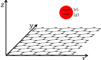
The model system considered in this paper is presented as a sketch in Fig.1. We consider an atomically thin monolayer of graphene in thexyplane, suspended in vacuum. Close to this graphene monolayer, we have either a single quantum system, when investigating spontaneous emission, or two quantum systems, for energy transfer investigations. We begin our investigation by considering a conductivity model for graphene and the GP properties.
A. Graphene conductivity and GP properties
We calculate the graphene in-plane conductivityσ in the random phase approximation (RPA) [34–36]. This quantity is mainly controlled by electron-hole pair excitation that can
FIG. 1. (Color online) A graphene monolayer in thexy plane, with the quantum emitter approximated as a two level system.
FIG. 2. (Color online) GP dispersion relation in doped graphene
ω(ks) for different values of the chemical potential μ; the dots show the quadratic approximation of the dispersion relation. The inset shows the propagation length of the GP modeLSPfor the same values of the chemical potentialμ.
be divided into intraband and interband excitations. It can be written as
σ =σintra+σinter, (1)
where the intraband and interband contributions are
σintra= 2ie
2t
π(+iγ)ln
2 cosh
1 2t
, (2)
σinter =
e2 4
1 2 +
1
π arctan
−2 2t
− i
2π ln
(+2)2 (−2)2+(2t)2
. (3)
In the above we have introduced the dimensionless parameters
=ω/μ,γ =ES/μ, andt=kBT /μ. Hereμis the chem-ical potential,T is the temperature, andES is the scattering energy. This scattering energy is related to the relaxation time
τ throughτ =/ES. Theσintraterm describes a Drude model response for intraband processes corrected with a term γ, which accounts for impurities compromising the electron’s mobility. Throughout this paper we consider a temperature
T =300 K and a value of the relaxation time of τ =1 ps [37,38]. Figure 2 shows the dispersion relation ω(ks) for different values of the chemical potentialμ, whereks is the in-plane wavevector. Due to the fact that retardation effects dominate for wave vectorsks> kFand energiesω >2μ, the GP dispersion curves in Fig.2terminate at these values, where
kF is the Fermi wave vector. When the chemical potential
μ has the value μ=0, the GM absorbance has the value
π α0≈2.3%, whereα0 is the fine structure constant. This is the asymptotic value of the doped GM for energiesω >2μ. Considering that the GM is surrounded by air,ε1=ε2=1 (free standing GM), the GP dispersion relation can be obtained from
1
k02−kSP2
= −2π σ
ω , (4)
[image:2.608.331.536.66.219.2] [image:2.608.88.257.622.723.2]contribution, to obtain
kSP=
2 4e2μk
BT ln
2 coshkμ BT
ω
ω+ i τ
, (5)
which has as its main feature the quadratic dependence of the GP wave vector on the frequency, when the intraband contributions dominate [34]. This approximate quadratic dependence is shown as dots in Fig. 2. Another feature of the GP dispersion relation on graphene is the fact that the GP resonance frequency is blueshifted as the chemical potential increases.
The inset in Fig. 2 shows the propagation length of the surface plasmon along the graphene LSP=1/Im(kSP), as a function of energy, for different values of the chemical poten-tialμ. It is evident from the plot that, depending on the value of the chemical potentialμ, this propagation length can reach values as large as hundreds of microns at low frequencies. As the energy is increased, however, the propagation length decreases rapidly, because the GP then has sufficient energy to generate electron-hole pairs and the dispersion relation is dominated by the interband contributions [3].
B. Rabi splitting—strong coupling regime
In order to ascertain whether the weak or strong coupling regime applies for particular sets of parameters, we now consider a model consisting of a single QE interacting with the GP mode of the GM. To describe this system we use a Jaynes-Cummings Hamiltonian [39] of the form
H =ω
2 σz+ωSPaˆ
†aˆ+g( ˆaσ
++aˆ†σ−), (6)
whereωSPis the GP frequency, ˆa†and ˆaare the creation and annihilation operators of the plasmon mode,ωis the transition frequency of the QE between its ground and excited state,σ+
andσ−are the raising and lowering operators of the QE, and
gis the coupling constant between the QE and the GP mode of the GM. The coupling constantgis given by [40]
|g(ω)|2= 1 π ε0
ω2
c2 ˆd
T
ImGSP(ω,rQE,rQE)ˆd
=γ03c ω ˆd
T
ImGSP(ω,rQE,rQE)ˆd, (7)
where GSP(ω,rQE,rQE) is the GP part of the Green’s tensor, derived in Appendix A [Eq. (A2a)], γ0 is the Einstein A coefficient, γ0=ω3d2/(3πε0c3), and d is the transition dipole moment of the QE positioned atrQE=(0,0,z). In this section we considerγ0=5×10⁻⁸fs−1 and we consider the transition dipole momentdof the QE to be oriented alongz. Since we are interested in the coupling between the GP mode and the QE we calculate the GP contribution to Eq. (A2a) by extracting the pole contribution and we obtain
G(11)SPS,zz (z,ω)= −1 4
(1−1/α2)
αk0 e
−2iz/α,
(8)
whereα=2π σ/c.
The Hamiltonian from Eq. (6) couples the states|e ⊗ |0 and|g ⊗ |1to the dressed states|1and|2with energies
E1= ωSP
2 − 2
δ2+4g2, (9a)
E2=
ωSP
2 + 2
δ2+4g2, (9b)
where δ=ωSP−ω is the detuning between the GP mode resonant frequency and the transition frequency of the QE. The energy states are separated by=δ2+4g2, which gives the value of the Rabi splitting. As an example, if we consider the case where the QE is positioned atz=10 nm above a GM with a chemical potential equal to the transition energy of the QE,μ=ω=0.5 eV, the Rabi splitting, atδ=0, has a value 2g(ω)=0.12 eV.
In order to further investigate the weak and strong coupling regimes, we will analyze the dependence of the coupling constant g on the various parameters involved, namely the value of the chemical potentialμ, the emission frequency of the QEω, and the distance of the QE to the GMz. Considering
ω=ωSP, i.e., zero detuning, the criterion for having strong coupling is whether or not the absorption spectrum of the system exhibits two peaks of different frequencies [40,41]. This condition is fulfilled if
|g|> 14|γLSW−κ|, (10)
whereγLSWrepresents thelossy surface waves(LSW) contri-bution, which are nonpropagating evanescent modes relaxing through ohmic losses, andκis the width of theg(ω)2spectrum. In Fig. 3(a) we present a contour plot of the quantity D=4|g|/|γLSW−κ|as a function of the chemical potential
μ and the emission energy ω for a fixed position of the QE,z=10 nm. Although from condition (10) whenD<1 we are in the weak coupling regime, this condition might not be sufficient under some experimental conditions [39], and we thus consider the more stringent inequalityD0.5 as giving the weak coupling condition. As is evident from Fig.3(a), for chemical potential valuesμ <0.3 eV there exists a frequency region where we have D0.5 and the weak coupling approximation needed to calculate the SE and ET rates is no longer valid. This region where the strong coupling dominates corresponds to THz frequencies, a range outside the scope of our investigation. For chemical potential values
FIG. 3. (Color online) Contour plots of the quantityD=4|g|/|γLSW−κ|as a function of (a) chemical potentialμand emission energy
ωnormalized by the chemical potential for fixed QE positionz=10 nm, and (b) chemical potentialμand QE positionz; each point reflects the maximum value ofD(ω).
III. RESULTS AND DISCUSSION A. Spontaneous emission rate
The decay rate γ is proportional to the strength of the coupling between the transition dipole matrix element and the electromagnetic modes acting on it. The normalized SE has the expression [27]
˜
γ = γ γ0 =
ni+
6π c
ω Im[nQE· Gs(r,r,ω)·nQE], (11)
whereγ0is Einstein’sAcoefficient,nQEis a unit vector along the direction of the transition dipole moment of the emitter, andG(r,r,ω) is given by (A2).
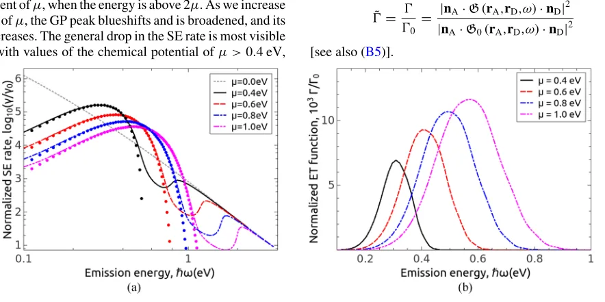
In Fig.4(a)we have plotted the normalized SE rate ˜γ of a QE at a fixed positionr=(0,0,10 nm) above the GM, as a function of the QE’s emission energyωfor different values of the chemical potentialμ. In general the SE rate has a peak at an energy belowμ. As the energy is further increased, the SE rate drops dramatically before finally recovering to a value independent ofμ, when the energy is above 2μ. As we increase the value ofμ, the GP peak blueshifts and is broadened, and its value decreases. The general drop in the SE rate is most visible starting with values of the chemical potential ofμ >0.4 eV,
and it occurs between the energies ω=μ and ω=2μ. This drop is due to interband transitions when the QE relaxes through lossy channels. At emission energies ω >2μ the emission is determined by interband contributions and GP excitations become unimportant, as the dispersion relations in Fig. 2 show. At these energies the SE rate follows the same behavior as for the case of undoped graphene μ=0 eV, as seen in Fig.4(a). Moreover, we can see that the main contribution to the peak in the normalized SE rate ˜γ comes from the GP contribution, which is denoted by the circular symbols in Fig. 4(a). The maximum value of D is 0.41 at
μ=0.4 eV, thus placing us within the weak coupling regime.
B. Energy transfer function
In this section we investigate the influence of the GM on the energy transfer process between a pair of QEs, a donor and an acceptor. The normalized energy transfer function which we investigate in this section is given as
˜
=
0
= |nA·G(rA,rD,ω)·nD|2
|nA·G0(rA,rD,ω)·nD|2
(12)
[see also (B5)].
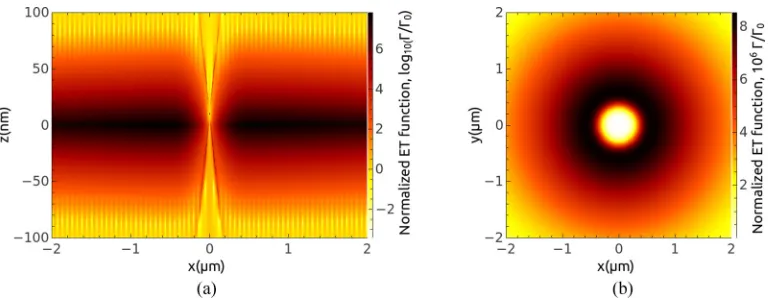
[image:4.608.89.522.66.223.2] [image:4.608.87.529.494.715.2]FIG. 5. (Color online) Contour plots of the normalized ET function in the (a)xzplane and (b)xyplane whenz=10 nm, for a donor positioned atrD=(0,0,10 nm) above a GM. The dielectric permittivity of the surrounding media isε1=ε2=1. The chemical potential of the graphene monolayer isμ=1.0 eV. The emission frequency of the donor isω=0.8 fs−1(λ=2.3μm). Both donor and acceptor have their transition dipole moments oriented along thezaxis.
Figure4(b)shows the normalized energy transfer function ˜
as a function of frequency for different values of the chemical potentialμ, and when both the donor and acceptor transition dipole moments are oriented perpendicular to the GM, i.e.,
zzorientation. The donor and acceptor positions are fixed at
rD=(0,0,10 nm) and rA=(100,0,10 nm), respectively. As for the case of the SE rate in Fig. 4(a), the normalized ET function ˜ is enhanced close to the GP frequency and in general for frequencies ω < μ, where the intraband tran-sitions dominate. For frequenciesω > μthe energy transfer rate decreases due to the losses generated by the interband contributions.
Figure 5 presents contour plots of the normalized ET function ˜ as a function of the position of the acceptor in (a) the xz plane and (b) the xy plane 10 nm above the GM, when the donor position is fixed at rD=(0,0,10 nm), the transition energy isω=0.52 eV (λ=2.3μm), and the chemical potential isμ=1.0 eV. In Fig.5(a)the normalized
ET function has large values when the acceptor is close to the GM and decreases as the acceptor distance is increased. This behavior is due to the fact that the field is highly confined in thezdirection at the surface of the GM, with a penetration depth ofδSP=10 nm, orδSP/λ=4×10−3. The fringes visible in Fig. 5(a) are due to the constructive and destructive interference between the direct and scattering terms in the Green’s tensor, cf. Eq. (A1). This effect is more profound due to the dipole moment orientations of the QEs, along thez
axis. Figure5(b)shows that the normalized ET function has cylindrical symmetry in thexyplane, due to the orientation of both donor and acceptor transition dipole moments along the
zaxis. Furthermore, we see that the normalized ET function has a peak value at a distance of about 400 nm, which is the propagation length of the GP mode for the particular set of parameters used in this calculation.
In Fig.6(a)we present thezdependence of the normalized ET function ˜ for a donor located at rD=(0,0,z) and an
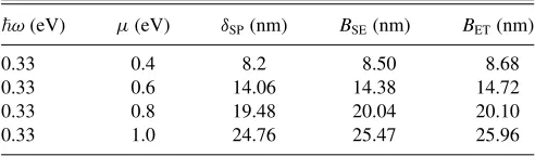
[image:5.608.114.498.67.216.2] [image:5.608.66.547.505.689.2]TABLE I. GP penetration depths.
ω(eV) μ(eV) δSP(nm) BSE(nm) BET(nm)
0.33 0.4 8.2 8.50 8.68
0.33 0.6 14.06 14.38 14.72
0.33 0.8 19.48 20.04 20.10
0.33 1.0 24.76 25.47 25.96
acceptor atrA=(100 nm,0,z), for various values of the chem-ical potential, and a fixed transition energy ω=0.33 eV. As we have already pointed out, for different values of the chemical potential μ, the position of the maximum in the normalized ET function blueshifts as the value of the chemical potential is increased, cf. Fig.4(b). Thus, for the smallest value of the chemical potentialμ=0.2 eV, the enhancement of the ET function is negligible to nonexistent. As the value of the chemical potential is increased, the ET function has values a few orders of magnitude larger than in free-space when the donor-acceptor pair is close to the GM. As the donor-acceptor pair is moved further from the GM—increasing z—the ET function drops off exponentially, as the figure shows. The continuous lines in Fig.6(a) represent fits of the calculated ET function (represented by symbols) with the exponential function Ae−4z/B. The factor 4 in this expression has two
sources: (i) the z distance of both donor and acceptor to the GM is varied and (ii) the ET function depends on the square of the field, see Eq. (12); each of these gives a doubling of the exponent, for a total of 2×2=4. Furthermore, because the donor-acceptor separation is kept constant at x=100 nm, the free-space ET function is also constant and, hence, does not influence the exponential behavior. Table I shows the values of the parameter BET extracted from the fit, together with the analogous parameterBSE extracted from fitting the SE dependence (the numerical factor in the exponent is 2 in this case, rather than 4, due to the fact that the SE rate depends linearly on the electric field; data not shown) and the penetration depth of the GP in the air above the graphene, calculated asδSP=1/Im(kSPz ). As this table shows, the values
of the parametersBSE andBET match closely the calculated penetration depths of the GPs. This suggests that the main channel for enhancing the ET function between the QEs is the GP resonance. As the separation between the two QEs becomes smaller and smaller, this relaxation channel becomes less and less important and the direct interaction dominates at distances belowx=20 nm, as Fig.6(b)shows. In Fig.6(b) we consider the influence of the in-plane distance between the donor and acceptor, for a fixed value of the chemical potential
μ=0.4 eV and fixed transition energy ω=0.33 eV. We again fit the calculated ET function data (symbols) with the expressionAe−4z/B. As one can see, abovex =50 nm theBET parameter extracted is very close to the penetration depth of the GP,δSP. When the donor and acceptor in-plane distance is smaller thanx =50 nm, the influence of the GP mode on the ET function is less profound, and, as the donor-acceptor pair is moved away from the GM, it recovers its free-space interaction at shorter distances. This is due to the fact that the influence of the homogeneous part of the Green’s tensor dominates over the scattered part, cf. Eq. (A1); this effect will
be further discussed in Sec.III C. In this section the quantity Dhas the largest value of 0.48 forμ=0.4 eV,ω=0.33 eV at a donor-GM distance of 8 nm, confirming that the system is in the weak coupling regime.
C. Energy transfer efficiency
In the previous section we investigated the SE and ET functions. When the donor dipole is excited it has two ways of relaxing to the ground state: it can either transfer its excitation energy to the acceptor dipole with an ET ratekET, or it can relax with decay ratekSE, where it is assumed that there is no nonradiative decay, i.e., the intrinsic quantum yield of the donor is Y0=1. The decay rate kSE takes account of photon emission into the far field, coupling to GP modes, and losses in the GM. The SE and ET processes are, therefore, in competition with each other and we introduce an energy transfer efficiency to describe this competition.
We define the energy transfer efficiencyηas
η= kET kSE+kET
. (13)
This quantity gives the relative contribution of the energy transfer process to the total decay rate of the donor. If the ET efficiencyηhas a valueη >50%, then the decay of the excited state of the donor occurs mainly by energy transfer to the acceptor, rather than relaxation into photon or GP modes.
We next consider a donor-acceptor pair. The donor emission and acceptor absorption spectra are both given by a Gaussian distribution
Aqe−(λ−λq)2/λ2q, (14)
where q =D represents the donor and q =A represents the acceptor. Aq is a normalization constant, λq gives the position of the spectral peak, and λq is related to the full width at half maximum (FWHM) of the spectrum. The donor emission peak and acceptor absorption maximum coincide atλD=λA=2μm. There are a variety of emitters at this wavelength, such as quantum dots and synthesized molecules [42,43]. The normalization constant of the donor emission spectrum fD(λ) is given as A−D1=
∞
0 dλfD(λ). The width of the spectrum will be λD=20 nm, a reasonable value for a typical QE. The normalization constant for the acceptor absorption spectrum isAA=0.021 nm2, while the width is
λAi =50 nm.
The F¨orster radius R0 is defined as the donor-acceptor separation at which the energy transfer efficiencyηis 50%.
R0 is calculated from the spectral overlap of the normalized donor emissionfDand acceptor absorptionσAspectra as
R0=
3c
32π4n4
r
∞
0
dλλ2fD(λ)σA(λ) 1/6
, (15)
wherenr is the refractive index of the host medium, in our case air withnr =1. For our case the F¨orster radius,R0, has a value of 19 nm in free space.
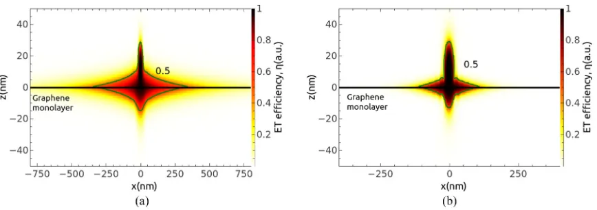
FIG. 7. (Color online) Contour plot of the ET efficiencyηbetween a pair of QEs, as a function of acceptor position for a fixed position of the donor atrD=(0,0,10 nm) and different values of the chemical potential, (a)μ=1 eV and (b)μ=0.6 eV. The green line gives the η=50% values.
When μ=1.0 eV the emission and absorption spectrum overlap strongly with the ET function. For this case the ET efficiencyηhas values above 70% even for separations along the GM as large as 100 nm, and the 50% efficiency distance is around 300 nm. This value is very large compared to the free-space F¨orster radius of R0=19 nm. When the value of the chemical potential is μ=0.6 eV, the ET efficiency
η has values above 50% for separations above 100 nm but now the overlap between the emission and absorption spectra and the ET function is poorer, thus showing a diminished effect. The large confinement of light at the atomically thin GM surface can be used to efficiently transfer energy between a pair of QEs over large separations. Furthermore, this ET efficiencyηcan be controlled through gating of the GM, thus opening striking opportunities for possible applications, such as switching and sensing devices [28–30], light harvesting [31], plasmonic rulers [29,32], and quantum computing [33].
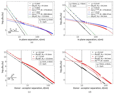
We next consider the behavior of the ET rate kET as a function of the in-plane separation between donor and acceptor. Figures 8(a) and 8(b) show the ET rate kET as a function of the in-plane separation between the donor and acceptor, when their elevation above the GM is (a) zD=
zA=5 nm and (b) zD=zA=10 nm on the same side of the GM. For both panels we have fitted the near field with a F¨orster-type model (R0/x)n, whereR0is the F¨orster radius. At small separations the fit yields the values n=6 typical of F¨orster ET, but we see that the F¨orster radius is modified from the free-space value. At small separationsx <10 nm, for zD=zA=5 nm andx <20 nm, for zD=zA=10 nm, the ET ratekETfollows ann=6 dependence showing that the homogeneous part of the Green’s tensor dominates, cf. (A1a), modified by the donor-acceptor interaction with the GM. Thus, there is an enhancement of the F¨orster radius, which depends on the donor-acceptor distances from the GM and the value of the chemical potentialμ. In Fig.8(a)the F¨orster radius has a value of R0=123.0 nm for chemical potential valuesμ=0.8 eV andμ=1.0 eV. As the chemical potential value drops, the F¨orster radius decreases to R0=91.0 nm for μ=0.4 eV, a value that is smaller than the one for the case of an undoped graphene layer R0≈100 nm, due to the interband transitions, cf. Fig. 4(a). The effect of tuning the F¨orster radius through the chemical potential is evident.
In Fig.8(b)the values of the F¨orster radius are smaller for the different values of the chemical potential μ due to the fact the QEs-GM distance is increased. Whenμ=1.0 eV we have the largest value of the F¨orster radiusR0=94.3 nm due to our choice of the donor and acceptor. For the off-resonance case μ=0.4 eV, the F¨orster radius is R0≈54.2 nm, once again smaller than the case of undoped grapheneR0≈70 nm. At larger donor-acceptor separations we use the following expression to fit the calculated ET rate:
f(x)=A
x exp
−2x
B
, (16)
which represents the dependence of the GP field intensity on the in-plane separationx (the factor 2 in the exponential results from the square of the Green’s tensor, as does the
x in the denominator—the GP field has a factor of 1/√x). The fitting parameter B is tabulated in Table II, together with the corresponding propagation length of the GP along the interface of the GM,LSP. As is clear, the correspondence between these parameters is very good indeed, confirming that, away from the near field, the interaction between donor and acceptor occurs primarily through the GP excited by the donor at the surface of the GM. As we increase the distance between the QEs and the GM, the F¨orster regime dominates further away from the near field, as can be seen from the fact that the intersection between the two fitting curves moves to larger distances. This is due to the small value of the penetration depth of the GP,δSP=6.6 nm atμ=1.0 eV. In the next paragraph we will further consider the influence of the penetration depth to the ET ratekET.
[image:7.608.90.524.67.220.2]Figures8(c)and8(d)consider the ET ratekETas a function of the donor-acceptor separation, for the case when the donor
TABLE II. GP propagation length.
z(nm) μ(eV) LSP(nm) B(nm)
5 0.8 379.23 376.82
5 1.0 890.31 884.86
10 0.8 379.23 376.99
[image:7.608.313.559.679.751.2]FIG. 8. (Color online) (a) and (b) ET ratekETas a function of the donor-acceptor in-plane separationxfor fixed donor positions (a)rD= (0,0,5 nm) and (b)rD=(0,0,10 nm), respectively, and variable acceptor positionrA=(x,0,5 nm) andrA=(x,0,10 nm), respectively, for different values of the chemical potentialμ. (c) and (d) ET ratekETas a function of the donor-acceptor separationdfor fixed donor positions (c)rD=(0,0,5 nm) and (d)rD=(0,0,10 nm), respectively, and variable acceptor positionrA=(0,0,zA), withd=zD−zAand for different values of the chemical potentialμ.
position is kept fixed at Fig. 8(c) zD=5 nm and Fig. 8(d)
zD=10 nm above the GM, and the separation between the donor-acceptor d =zD−zA is varied, for μ=1.0 eV and
μ=0.4 eV. At small separations we again use the F¨orster model fitting presented earlier. To fit the behavior of the ET rate
kETbelow the GM we choose the expressionf(z)=Ae−2z/B,
where the parameterBwill be connected with the penetration depth of the GP, δSP. In both figures the GM position is denoted by the dashed vertical line. In Fig. 8(c), for which the donor position is very close to the GM (zD=5 nm), the behavior of the ET rate immediately below the GM is not trivial and comes from various contributions, such as direct interaction and GP coupling. On the other hand, in Fig.8(d), for whichzD=10 nm, we can use the fitting functionf(zA), and find for B the value B=δSP=6.6 nm, showing that the main contribution to the ET rate comes from the GP on the GM. For theμ=0.4 eV case the ET ratekET is almost uninfluenced by the presence of the GM. The quantityDhas a
maximum value of 0.2 for the donor-GM distance of 5 nm and
μ=1.0 eV.
IV. SUMMARY AND CONCLUSIONS
We have considered in this contribution the behav-ior of quantum systems placed near a free-standing graphene monolayer. The graphene monolayer can support graphene surface plasmon modes, tightly confined to the surface and having large propagation distances along the graphene monolayer.
We have begun by investigating the conditions of strong and weak coupling between a quantum system and the surface plasmon-polariton on the graphene monolayer. We have seen that for reasonably large values of the chemical potential
[image:8.608.71.537.66.451.2]and energy transfer functions. We have found that both of these quantities are enhanced, compared to their free space values, due to efficient coupling to the graphene plasmon modes.
Due to the competition of the donor-acceptor energy transfer process with other donor decay processes, we have defined the energy transfer efficiencyηand have investigated the influence of the graphene plasmons on this quantity. We have shown that the energy transfer efficiency η can reach values above 50% for distances up to 300 nm along the graphene monolayer. This process can be controlled by tuning the value of the chemical potential, e.g., through gating.
Finally, we investigate the ET ratekET varying the donor-acceptor in-plane separation and distance from the GM, for various values of the chemical potentialμ. The ET rate, when the in-plane distance between the donor and acceptor is varied, has two major contributions: the F¨orster-type mechanism dominates at small separations, while the GP contribution dominates at large distances. The F¨orster-type ET rate follows a x−6 dependence, with an increased F¨orster radius value, due to the presence of the GM. The F¨orster radius value is increased from a value of R0=91.0 nm whenμ=0.4 nm, to R0=123.0 nm when zD=zA=5 nm and μ=1.0 eV. At larger distances, the main contribution comes from the GP propagation; the transition from the F¨orster to the GP-propagation mechanism depends on the distance of the donor-acceptor pair from the GM, and it occurs at donor-donor-acceptor separations ranging from a few nanometers to a couple of tens of nanometers. When thezdistance between donor-acceptor is varied, forx=0, the behavior is somewhat more complicated, but the GP penetration depth still dictates the interaction length. As the chemical potential μ decreases the ET rate approaches the value for the case of undoped graphene. Thus, by varying the value of the chemical potential, we can tune the interaction channel or preferentially couple different species of resonant donor-acceptor pairs of QEs.
ACKNOWLEDGMENT
This work was supported by Science Foundation Ireland under Grant No. 10/IN.1/12975.
APPENDIX A: GREEN’S TENSOR FORMALISM We will consider two planar half-spaces with different dielectric permittivitiesε1 andε2. Thezdirection is perpen-dicular to the boundary between the two half-spaces. In order to calculate the Green’s tensor for this system, we use the method of scattering superposition [44]. The Green’s tensor has the form
G(11)(r,s,ω)=G(11)h (r,s,ω)+G(11)s (r,s,ω), (A1a)
G(21)(r,s,ω)=G(21)s (r,s,ω), (A1b)
where the first of the two labels in the superscript (i1) denotes the field point, while the second denotes the source point. The subscriptsdenotes the scattering term, always present, while the homogeneous termG(11)h (r,s,ω) contributes only when the source and field points are in the same medium.
The scattering terms have the following expression:
G(11)s (r,s,ω)= i 8π2
K
d2kρ 1 kz1kρ2
RK+11−K(kρ,kz1,r)
⊗K∗(kρ,−kz1,s), (A2a)
G(21)s (r,s,ω)= i 8π2
K
d2kρ 1 kz1kρ2
R−K11−K(kρ,−kz2,r)
⊗K∗(kρ,−kz1,s), (A2b)
where kρ=√k2
i −kzi2 is the in-plane propagation constant, kzi is the perpendicular propagation constant in medium i,
andki= ωc√εi is the wave number in medium i (i=1,2).
The above expressions involve a summation over K which represents M and N, or the transverse electric (TE) and transverse magnetic (TM) modes.
We impose the following continuity conditions at the boundary between the two half-spaces,z=0:
ˆ
z×[G(11)(r,s,ω)−G(21)(r,s,ω)]z=0=0, (A3a)
ˆ
z×∇×G(11)(r,s,ω)−∇×G(21)(r,s,ω)z=0
= −i4π
c k0σzˆ×zˆ×G
(21)(r,s,ω), (A3b)
whereσis the surface conductivity.
Using Eqs. (A2) in (A3) we obtain the generalized Fresnel coefficients, which have the form [13,45]
RM11 =kz1−kz2−2αk0 kz1+kz2+2αk0
,
(A4a)
RN11 =k
2
2kz1−k21kz2+2αk0kz1kz2
k2
2kz1+k21kz2+2αk0kz1kz2
,
RM21 = 2kz1 kz1+kz2+2αk0
,
(A4b)
RN21 = 2k1k2kz1
k22kz1+k21kz2+2αk0kz1kz2
,
whereα=2π σ/c.
APPENDIX B: SPONTANEOUS EMISSION AND ENERGY TRANSFER RATES
The spontaneous emission functionγ has the form [46,47]
γ(r,ω)= 2ω 2μ2
ε0c2Im[nμ·G(r,r,ω)·nμ], (B1) wherenμis a unit vector along the direction of the transition dipole moment of the emitterμandG(r,r,ω) is the Green’s tensor introduced in AppendixA.
A useful quantity to introduce is the normalized SE rate, defined as
˜
γ = γ γ0
=ni+
6π c
ω Im[nμ· Gs(r,r,ω)·nμ], (B2)
which we introduced in Eqs. (A1) and ni= √εi is the refractive index of the medium into which the quantum system is embedded. The normalized SE rate gives either an enhancement ( ˜γ >1) or a reduction ( ˜γ <1) of the SE rate compared to its free-space valueγ0.
When dealing with statistical ensembles of emitters, the emission spectrum will be different from that of a single emitter, which we have taken to have aδshape. The emission rate for the ensemble can then be expressed as
kSE=
∞
0
dλfD(λ)γ(λ), (B3)
wherefD(λ) is the area-normalized emission spectrum of the emitter, with0∞dλfD(λ)=1.
Furthermore, we introduce the ET function between a donor-acceptor pair, which has the form [27]
(rA,rD,ω)= 2π
2
ω2
c2ε 0
2
|μA·G(rA,rD,ω)·μD|2, (B4)
where againG(rA,rD,ω) is the Green’s tensor for the particular geometry,rD(A) is the position of the donor D (acceptor A), and μD(A) is the transition dipole moment of the donor D (acceptor A). The above expression for the energy transfer function depends on the donor-acceptor pair through the emission frequency of the donor and the transition dipole moment of the donor and acceptor. The influence of the
geometry is completely encapsulated in the Green’s tensor, being proportional to the electric field intensity, through the square of the Green’s tensor.
To consider only the influence of the geometry on a general donor-acceptor pair, we now introduce the normalized ET function for the system ˜defined as
˜
(ω)= (ω)
0(ω) =
|nA·G(rA,rD,ω)·nD|2
|nA·G0(rA,rD,ω)·nD|2
, (B5)
where G0(rA,rD,ω) is the Green’s tensor in free space and
nD(A)is a unit vector in the direction ofμD(A).
Analogously to the case of the SE rate, when considering statistical ensembles of donors and acceptors, the donor emis-sion spectrum fD(λ) and acceptor absorption cross-section
σA(λ) need to be taken into account when calculating the energy transfer rate. We therefore have [26]
kET=36π2YDkSE ∞
0 dλ
λ2fD(λ)|nA·G(rA,rD,λ)·nD| 2σ
A(λ),
(B6)
where YD is the intrinsic quantum yield of the donor. We have used this expression to calculate the energy transfer rate between donors and acceptors with specific emission and absorption spectra and to investigate how the energy transfer process competes with the emission process of the donor.
[1] W. L. Barnes, A. Dereux, and T. W. Ebbesen,Nature (London) 424,824(2003).
[2] J. A. Dionne, L. A. Sweatlock, H. A. Atwater, and A. Polman, Phys. Rev. B72,075405(2005).
[3] F. J. Garc´ıa de Abajo,ACS Photon.1,135(2014).
[4] A. N. Grigorenko, M. Polini, and K. S. Novoselov,Nat. Photon. 6,749(2012).
[5] P. Alonso-Gonz´alez, A. Y. Nikitin, F. Golmar, A. Centeno, A. Pesquera, S. V´elez, J. Chen, G. Navickaite, F. Koppens, A. Zurutuza, F. Casanova, L. E. Hueso, and R. Hillenbrand,Science 344,1369(2014).
[6] Y. V. Bludov, A. Ferreira, N. M. R. Peres, and M. I. Vasilevskiy, Int. J. Mod. Phys. B27,1341001(2013).
[7] T. Low and P. Avouris,ACS Nano8,1086(2014).
[8] A. H. Castro Neto, N. M. R. Peres, K. S. Novoselov, and A. K. Geim,Rev. Mod. Phys.81,109(2009).
[9] R. R. Nair, P. Blake, A. N. Grigorenko, K. S. Novoselov, T. J. Booth, T. Stauber, N. M. R. Peres, and A. K. Geim,Science320, 1308(2008).
[10] S. Thongrattanasiri, F. H. L. Koppens, and F. J. Garc´ıa de Abajo, Phys. Rev. Lett.108,047401(2012).
[11] V. W. Brar, M. S. Jang, M. Sherrott, J. J. Lopez, and H. A. Atwater,Nano Lett.13,2541(2013).
[12] A. Y. Nikitin, F. Guinea, F. J. Garc´ıa-Vidal, and L. Mart´ın-Moreno,Phys. Rev. B85,081405(2012).
[13] G. W. Hanson,J. Appl. Phys.103,064302(2008).
[14] A. Y. Nikitin, F. Guinea, F. J. Garc´ıa-Vidal, and L. Mart´ın-Moreno,Phys. Rev. B84,195446(2011).
[15] K. A. Velizhanin and A. Efimov, Phys. Rev. B 84, 085401 (2011).
[16] G. G´omez-Santos and T. Stauber, Phys. Rev. B 84, 165438 (2011).
[17] F. H. L. Koppens, D. E. Chang, and F. J. Garc´ıa de Abajo,Nano Lett.11,3370(2011).
[18] J. Tisler, T. Oeckinghaus, R. J. St¨ohr, R. Kolesov, R. Reuter, F. Reinhard, and J. Wrachtrup,Nano Lett.13,3152(2013). [19] G. Konstantatos, M. Badioli, L. Gaudreau, J. Osmond, M.
Bernechea, F. P. Garcia de Arquer, F. Gatti, and F. H. L. Koppens, Nat. Nanotechnol.7,363(2012).
[20] A. Manjavacas, S. Thongrattanasiri, D. E. Chang, and F. J. Garc´ıa de Abajo,New J. Phys.14,123020(2012).
[21] A. Gonzalez-Tudela, D. Martin-Cano, E. Moreno, L. Mart´ın-Moreno, C. Tejedor, and F. J. Garc´ıa-Vidal, Phys. Rev. Lett. 106,020501(2011).
[22] D. Dzsotjan, A. S. Sørensen, and M. Fleischhauer,Phys. Rev. B 82,075427(2010).
[23] P. A. Huidobro, A. Y. Nikitin, C. Gonz´alez-Ballestero, L. Mart´ın-Moreno, and F. J. Garc´ıa-Vidal,Phys. Rev. B85,155438(2012). [24] S.-A. Biehs and G. S. Agarwal,Appl. Phys. Lett.103,243112
(2013).
[25] K. A. Velizhanin and T. V. Shahbazyan,Phys. Rev. B86,245432 (2012).
[26] X. Zhang, C. A. Marocico, M. Lunz, V. A. Gerard, Y. K. Gun’ko, V. Lesnyak, N. Gaponik, A. S. Susha, A. L. Rogach, and A. L. Bradley,ACS Nano8,1273(2014).
[27] H. T. Dung, L. Kn¨oll, and D.-G. Welsch, Phys. Rev. A65, 043813(2002).
[28] F. Schwierz,Nat. Nanotechnol.5,487(2010).
Cataliotti, F. Koppens, and C. Toninelli,New J. Phys.16,113007 (2014).
[30] Q. He, S. Wu, Z. Yin, and H. Zhang,Chem. Sci.3,1764(2012). [31] C.-C. Lin, D.-Y. Wang, K.-H. Tu, Y.-T. Jiang, M.-H. Hsieh, C.-C.
Chen, and C.-W. Chen,Appl. Phys. Lett.98,263509(2011). [32] Y. Wang, Z. Li, J. Wang, J. Li, and Y. Lin,Trends Biotechnol.
29,205(2011).
[33] M. J. Gullans and J. M. Taylor,arXiv:1407.7035.
[34] M. Jablan, H. Buljan, and M. Soljaˇci´c,Phys. Rev. B80,245435 (2009).
[35] B. Wunsch, T. Stauber, F. Sols, and F. Guinea,New J. Phys.8, 318(2006).
[36] L. A. Falkovsky,J. Phys.: Conf. Ser.129,012004(2008). [37] K. S. Novoselov, A. K. Geim, S. V. Morozov, D. Jiang, Y. Zhang,
S. V. Dubonos, I. V. Grigorieva, and A. A. Firsov,Science306, 666(2004).
[38] K. S. Novoselov, A. K. Geim, S. V. Morozov, D. Jiang, M. I. Katsnelson, I. V. Grigorieva, S. V. Dubonos, and A. A. Firsov, Nature (London)438,197(2005).
[39] P. T¨orm¨a and W. L. Barnes, Rep. Prog. Phys. 78, 013901 (2015).
[40] T. H¨ummer, F. J. Garc´ıa-Vidal, L. Mart´ın-Moreno, and D. Zueco, Phys. Rev. B87,115419(2013).
[41] L. C. Andreani, G. Panzarini, and J.-M. G´erard,Phys. Rev. B 60,13276(1999).
[42] J. M. Pietryga, R. D. Schaller, D. Werder, M. H. Stewart, V. I. Klimov, and J. A. Hollingsworth,J. Am. Chem. Soc.126,11752 (2004).
[43] J. A. Treadway, G. F. Strouse, R. R. Ruminski, and T. J. Meyer, Inor. Chem.40,4508(2001).
[44] W. C. Chew,Waves and Fields in Inhomogeneous Media(IEEE, New York, 1995).
[45] A. Y. Nikitin, F. J. Garc´ıa-Vidal, and L. Mart´ın-Moreno,IEEE J. Select. Topics Quantum Electron.19,4600611(2013). [46] H. T. Dung, L. Kn¨oll, and D.-G. Welsch,Phys. Rev. A57,3931
(1998).