A unified closed loop stability measure for finite precision digital controller realizations implemented in different representation schemes

A Unified Closed-Loop Stability Measure for Finite-Precision Digital Controller Realizations Implemented in Different Representation Schemes

Jun Wu, Sheng Chen, James F. Whidborne, and Jian Chu

Abstract—A computationally tractable unified finite word length closed-loop stability measure is derived which is applicable to fixed-point, floating-point and block-floating-point representation schemes. Both the dynamic range and precision of an arithmetic scheme are considered in this new unified measure. For each arithmetic scheme, the optimal controller realization problem is defined and a numerical optimization approach is adopted to solve it. Numerical examples are used to illustrate the design procedure and to compare the optimal controller realizations in different representation schemes.

Index Terms—Closed-loop stability, digital controller, finite word length, number representation format, optimization.

I. INTRODUCTION

In recent years, there has been a growing interest in digital controller implementation which reduces the finite word length (FWL) effects on closed-loop stability (see [1], [2], and the references therein). It is well known that a control law can be accomplished with different re-alizations and that the parameters of a controller realization are repre-sented by a digital processor of finite bit length in a particular format, namely fixed-point, floating-point, or block-float-point format. Pre-vious works [3]–[8] have derived various FWL closed-loop stability measures for these three formats separately and defined corresponding optimal controller realization problems based on these measures. How-ever, all these previous measures are only linked to the precision bits of the respective representation schemes used and they do not consider the dynamic range bits. Arguably, a better approach is to consider some measure which has a direct link to the total bit length required. The main contribution of this note is to derive a unified FWL closed-loop stability measure that can accommodate both the dynamic range and precision requirements and is applicable to all the three schemes.

II. REPRESENTATIONSCHEMES

The fixed-point format with a bit length = 1+g+frepresents a real numberx 2 R by assigning 1 bit for the sign, gbits for the integer part, andfbits for the fraction part ofx. Assuming no overflow, which means thatjxj 2 ,x is perturbed to

Q1(x) = x + 1 j1j < 20( +1): (1)

Anyx 2 R can be expressed uniquely as x = (01)s2 w 2 2e, wheres 2 f0; 1g is the sign of x, w 2 [0:5; 1) is the mantissa of x, e = blog2jxjc + 1 2 Z is the exponent of x, Z denotes the set of integers and the floor functionbxc is the closest integer less than or

Manuscript received January 18, 2002; revised September 30, 2002. Rec-ommended by Associate Editor D. E. Miller. The work of J. Wu and S. Chen was supported by the U.K. Royal Society under a KC Wong Fellowship (RL/ART/CN/XFI/KCW/11949). The work of J. Wu and J. Chu was supported by the National Natural Science Foundation of China under Grant 60174026.

J. Wu and J. Chu are with the National Key Laboratory of Industrial Con-trol Technology Institute of Advanced Process ConCon-trol Zhejiang University, Hangzhou 310027, China.

S. Chen is with the Department of Electronics and Computer Science Uni-versity of Southampton, Highfield, SO17 1BJ Southampton, U.K.

J. F. Whidborne is with the Department of Mechanical Engineering King’s College London, Strand, WC2R 2LS London, U.K.

Digital Object Identifier 10.1109/TAC.2003.811260

equal tox. The floating-point format with a bit length = 1+w+e representsx by assigning 1 bit for s, wbits forw and ebits fore. Lete and e be the lower and upper limits of the exponent, respectively. Clearly,e 0 e = 2 0 1. Denote the set of integers e e e as Z[e;e]. Assuming that no underflow or overflow occurs, which means that the exponent ofx is within Z_[e;e],x is perturbed to [7]

Q2(x) = x + x2 j2j < 20( +1): (2) In the block-floating-point format, a set of real numbersS is first divided into some blocks. For an illustrative purpose, consider the case of dividingS into the two nonempty and nonoverlapped subsets S1and S2. Let12 S1be the element inS1that has the largest absolute value, and2 2 S2 be the element inS2that has the largest absolute value. Then, anyx 2 S can be expressed uniquely as x = (01)s2 u 2 2h, whereu 2 [0; 1) is the block mantissa of x, and the block exponent of x is

h=1 blog2j1jc + 1; for x 2 S1

blog2j2jc + 1; for x 2 S2: (3)

When all the elements inS are presented in the block-floating-point format of bit length = 1 + _u+ _h, the bits are assigned as follows: 1 bit for the sign,ubits foru which is represented in fixed-point with the two’s complement system, and_h bits forh. Let h and h be the lower and upper limits of the block exponent, respectively. Obviously, h 0 h = 2 _{0 1. Denote}

r(x)=1 2₂1; for x 2 S1

2; for x 2 S2: (4)

Assuming no underflow or overflow, i.e., the block exponent ofx is withinZ_[h;h], it can be shown thatx is perturbed to

Q3(x) = x + r(x)3 j3j < 20( +1): (5) It is easily seen that in each representation format the total bit length always consists of three parts. Sign occupies one bit. The dynamic range of representation is defined by_g,_e, or_hbits, and the preci-sion of representation is determined byf,w, orubits, depending on which scheme is actually chosen. For notational conciseness, we introduce the “generalized” dynamic range bit lengthrand precision bit lengthpfor the three representation schemes. It is understood that r = g,e, orh andp = f,w oru, depending on which format is actually used.

III. PROBLEMSTATEMENT

The discrete-time linear time-invariant plantP is described by x(k + 1) = Ax(k) + Be(k)

y(k) = Cx(k) (6)

withA 2 Rn2n,B 2 Rn2p, andC 2 Rq2n. The generic digital controllerC is described by

v(k + 1) = Fv(k) + Gy(k) + He(k)

u(k) = Jv(k) + My(k) (7)

withF 2 Rm2m,G 2 Rm2q,J 2 Rp2m,M 2 Rp2q, andH 2 Rm2p_{. Lete(k) = q(k) + u(k) with the command input q(k). Then,} P and C form a discrete-time closed-loop control system.

Assume that a realization (F0,G0,J0,M0,H0) ofC has been designed. It is well-known that the realizations ofC are not unique. All the realizations ofC form the realization set

Sc= (F; G; J; M; H) : F = T1 01F0T; G = T01G0

J = J0T; M = M0; H = T01H0 (8) whereT 2 Rm2m is any real-valued nonsingular matrix, called a similarity transformation. Letw_F=Vec(F), where Vec(1) denotes the1

column stacking operator. The vectorswF ,wG,wG ,wJ,wJ ,wM, wM ,wH, andwH are similarly defined. Denote

w = [w11 1 1 wN]T 1= wFTwTGwTJwMTwTH T

;

w0= w1 TF wTG wTJ wTM wTH (9)

whereN = (m+p)(m+q)+mp andT is the transpose operator. We also refer tow as a realization of C. The stability of the closed-loop system depends on the eigenvalues of the matrix

A(w)=1 _{GC + HMC F + HJ}A + BMC BJ

= _{0 T}I 0₀₁ A(w0) _{0 T}I 0 (10)

where0 and I denote the zero and identity matrices of appropriate dimensions, respectively. All the different realizationsw have the same set of closed-loop poles if they are implemented with infinite precision. Since the closed-loop system is designed to be stable, the eigenvalues ji(A(w))j = ji(A(w0))j < 1; 8i 2 f1; . . . ; m + ng.

Define the index of representation formats

=

1; fixed-point format is adopted 2; floating-point format is adopted 3; block-floating-point format is adopted:

(11)

The controller realizationw is implemented in format of rdynamic range bits,_pprecision bits and one sign bit. In the remainder of this note, it is assumed that ifw is stored in the block-floating-point format, it is divided into “natural” blocks ofwF,wG,wJ,wM andwH. Let F 2 wF be the element inF which has the largest absolute value. The elementsG,J,MandHare similarly defined. Denote

kwkmax1= max j2f1;111;Ngjwjj

(w)=min1 j2f1;111;Ngfjwjj : wj 6= 0g

z(w)=[1 FGJMH]T: (12)

Firstly, the dynamic range ofrbits must be large enough forw. We define a dynamic range measure for controller realizationw in format as

(w; )=1

kwkmax; = 1

log₂ 4kwk

(w) ; = 2

log2 4kz(w)k(z(w)) ; = 3

: (13)

Proposition 1: The realizationw can be represented in format of rdynamic range bits without overflow( = 1) or without underflow or overflow ( = 2; 3), if 2 (w; ).

Proof: The proof is straightforward. Here, we only give the case of = 3. When 2 log₂(kz(w)kmax=(z(w))) + 2, we have

2 _{0 1 log}

2 kz(w)k_(z(w))max + 1 log2kz(w)kmax + 1

0 (blog₂ (z(w))c + 1) : (14)

According to the results of Section II, this means thatF, G, J, M andHcan all be represented without underflow or overflow and, therefore,w can be represented in the block-floating-point format of hblock exponent bits without underflow or overflow.

Letmin_r be the smallest dynamic-range bit length that, when used to implementw, does not cause overflow or underflow. This minimum dynamic-range bit length can easily be computed by

rmin(w; ) =

dlog₂kwkmaxe; =1

dlog₂(blog₂kwkmaxc0blog2(w)c+1)e; =2 dlog₂(blog₂kz(w)kmaxc0blog2(z(w))c+1)e; =3

(15)

where the ceiling functiondxe denotes the closest integer greater than or equal tox 2 R. Note that the measure (w; ) defined in (13) provides an estimate of_rminas ^_rmin(w; )=dlog1 ₂(w; )e. It can easily be seen that ^_rmin _rmin.

For a vectorx, let d(x) be the vector of the same dimension whose elements are all 1’s, and denote

(x)=1 0; x is a zero vector_{1; x is a nonzero vector}: (16)

For two vectorsx = [xj] and y = [yj] of the same dimension, define the Hadamard product ofx and y as x y=[x1 jyj]. When the dynamic range is sufficient, according to the results of Section II,w is perturbed tow + r(w; ) 1 due to finite pwhere

r(w; 1) =

(wF)d(wF) (wG)d(wG) (wJ)d(wJ) (wM)d(wM)

(wH)d(wH) r(w; 2) = w

r(w; 3) =

2Fd(wF) 2Gd(wG) 2Jd(wJ) 2Md(wM)

2Hd(wH)

: (17)

Each elementjof1 is bounded by 620( +1), that is,k1kmax < 20( +1)_{. With the perturbation1,}

i(A(w)) is moved to i(A(w+ r(w; ) 1)). If an eigenvalue of A(w + r(w; ) 1) is outside the open unit disk, the closed-loop system, designed to be stable, becomes unstable with the finite-precision implementedw. Therefore, it is crit-ical to know when the FWL error will cause closed-loop instability. This means that we would like to know the largest open “hypercube” in the perturbation space within which the closed-loop system remains stable. Based on this consideration, a precision measure for realization w of format can be defined as

0(w; )= inf k1k1 max: A (w + r(w; ) 1) is unstableg : (18) From the previous definition, the following proposition is obvious.

Proposition 2: A(w + r(w; ) 1) is stable if k1kmax < 0(w; ).

Thus, under the condition that the dynamic range is sufficient, that is, _{r r}min, the perturbationk1k_max and therefore the preci-sion bit lengthpdetermines whether the closed-loop remains stable. Letmin_p be the smallest precision bit length such that8_{p p}min, the closed-loop system is stable withw implemented by pprecision bits. The precision measure0(w; ) provides an estimate of pminas

^ min

p0 (w; )=0blog1 20(w; )c01. It can be seen that ^minp0 pmin. Define the minimum total bit length required in the implementa-tion ofw as min 1=min_r + _pmin+ 1. Clearly, w implemented with a bit length min can guarantee a sufficient dynamic range and closed-loop stability. Combining the measures(w; ) and 0(w; ) results in the following true FWL closed-loop stability measure for the given realizationw with format

0(w; )1= _{(w; )}0(w; ): (19)

An estimate of min is given by 0(w; ) as ^0min(w; )= 01 blog20(w; )c + 1. It is clear that ^min0 min. The following proposition summarizes the usefulness of0(w; ) as a measure for the FWL characteristics ofw in representation format .

Computing the value of0(w; ), however, is an unsolved open problem. Thus, the true FWL closed-loop stability measure0(w; ) has limited practical significance. In the next section, an alternative measure is developed which not only can quantify FWL characteristics ofw in format but also is computationally tractable.

IV. A TRACTABLEFWL CLOSED-LOOPSTABILITYMEASURE AND ITSOPTIMIZATION

First,8i 2 f1; . . . ; m + ng

i A (w+r(w; ) 1) = i A(w) + G

@jij

@1 d1 (20)

where G is the oriented curve from 0 to 1. For the derivative (@jij)=(@1) = [(@jij)=(@j)], define

@jij @1 ₁=1

N

j=1 @jij

@j : (21)

Further define the precision measure for realizationw in format

i(w; )=1 min i2f1;111;m+ng

1 0 i A(w) @j j

@1 1=0 1

: (22)

Obviously, ifk1k_max < ₁(w; ) and

i A (w + r(w; ) 1)

0 i A(w) k1kmax @j_@1ij 1=0 1

(23)

thenji(A(w+r(w; )1))j < 1 which means that the closed-loop remains stable under the FWL error1. As discussed in [5] and [6], the condition (23) is satisfied, provided that₀(w; ) is small enough. The assumption of small0(w; ) is generally valid, as it does not make much sense to study the FWL effects on the closed-loop stability for those situations where the closed-loop systems have a very large sta-bility robustness. Hence, (23) is not restrictive. Thus, with a sufficient dynamic range, the closed-loop can tolerate those FWL perturbations 1 whose norms k1kmaxare less than1(w; ). Similar to 0(w; ), from the precision measure₁(w; ), an estimate of _pminis given as

^ min

p1 (w; )= 0 blog1 21(w; )c 0 1.

Comment: In (20), G should be chosen to avoid those points where derivative (@jij)=(@1) do not exist, and the derivative (@jij)=(@1)j1=0 must exist. From the results of [5] and [6], (@jij)=(@1)j1=0 exist if A(w) has m + n distinct nonzero eigenvalues. IfA(w) has multiple repeating closed-loop eigenvalues, some of(@j_ij)=(@1)j₁₌₀may not exist, and in this case₁(w; ) is not defined. However, in practical control system designs, it is very rare that A(w) has multiple repeating eigenvalues. As for the case ofi = 0, since the zero eigenvalue has the largest stability margin 1 0 jij, it is harder to move across the unit circle under the FWL effects, compared with the other nonzero eigenvalues. Hence, for thoseA(w) having zero eigenvalue, 1(w; ) may be modified such that it only minimizes(1 0 j_i(A(w))j)=(k@(j_ij)=(@1)j₁₌₀k₁) for those nonzero eigenvalues. Alternatively, the more conservative measures of [4] and [5] could be used for cases where there are zero eigenvalues.

Obviously, 1(w; ) is an approximation of 0(w; ). How-ever, unlike the measure 0(w; ), the value of 1(w; ) can be computed explicitly. It is easy to see that (@jij)=(@1)j1=0 = r(w; ) (@jij)=(@w) and from the results of [6], it can be shown that

@ i A(w)

@F =[0 I]Li(w) 0I

@ i A(w)

@G =[0 I]Li(w) C T 0 @ i A(w)

@J =[BT HT]Li(w) 0I @ i A(w)

@M =[BT HT]Li(w) C T 0 @ i A(w)

@H =[0 I]Li(w) C T_MT

JT (24)

with

Li(w)=1Re 3

i A(w) yi3 A(w) pTi A(w) i A(w)

(25)

wherepi(A(w)) and yi(A(w)) are the right and reciprocal left eigen-vectors related toi(A(w)), respectively,3denotes the conjugate op-eration andRe[1] the real part. Replacing 0(w; ) with 1(w; ) in (19) leads to a computationally tractable FWL closed-loop stability measure

1(w; )= 1 _{(w; )}1(w; ): (26)

From 1(w; ), an estimate of min is given as ^₁min(w; )= 01 blog₂1(w; )c + 1. Compared with the existing FWL measures [1]–[8],1(w; ) has at least two advantages. First, 1(w; ) can be used in different representation formats while the existing measures are only valid for a particular format. For example, the measures presented in [3]–[6] are fixed-point measures and the measure in [7] is a floating-point one. The measure1(w; ) offers a unified framework to compare the FWL characteristics of a realization w in different formats. Second and more critically, unlike the existing measures which are precision measures only and imply an unlimited dynamic range,1(w; ) is made up of a dynamic range measure and a precision measure and is therefore a true FWL measure capable of handling closed-loop stability as well as the underflow and overflow aspects.

In a given format, different realizations w yield different values of 1(w; ). It is of practical importance to find an “optimal” realization wopt() that maximizes 1(w; ) for the format . The controller implemented with this optimal realizationwopt() in format needs a minimum bit length and has a maximum tolerance to the FWL error. This optimal realization problem is formally defined as

v()= max1

w2S 1(w; ): (27)

Considering thatw is a function of T, r(w; ) and (w; ) depend on T and , we can define the following optimization criterion in format :

(T; )=1 min i2f1;111;m+ng

1 0 i A(w0) r(w; ) @j j

@w ₁(w; )

= 1(w; ): (28)

The optimal realization problem (27) can then be posed as the following optimization problem:

v() = max (T; ): (29)

as Rosenbrock and Simplex algorithms [11], are computationally sim-pler but run more risks of only attaining a local solution. Our expe-rience with the optimization problem (29) suggests that, unlike opti-mizing the precision measure₁(w; 1) alone [6], the dynamic range measure(w; ) in the criterion 1(w; ) helps to bound the solution set and the cost function(T; ) appears to behave better. It also help to choose a “good” initial controller realization, such as the open-loop balanced realization [12] or Li’s closed-loop suboptimal realization [4], as the initial guess for the optimization routine.

WithTopt(), the corresponding optimal realization wopt() in format can readily be computed. By setting = 1; 2; 3, respectively, in the optimization problem (29), we can attain an optimal fixed-point realizationwopt(1), an optimal floating-point realizationwopt(2) and an optimal block-floating-point realizationwopt(3) for a digital con-troller. It is worth reiterating that the optimization problem (29) yields a true optimal controller realization, as the solutionTopt() minimizes the requiredp as well asr and, therefore, minimizes the required total bit length. This should be compared with the existing “optimal” realization problems [1]–[8], which only try to minimize the required precision bitpand, as a consequence, do not necessarily minimize the required total bit length.

It is interesting to compare our approach with eigenstructure orthog-onalization, which is also based on eigenvalue sensitivities [1]. For a complex-valued matrixU, let kUk₂represent its largest singular value. The following lemma summarizes three properties ofk 1 k2.

Lemma 1: kUk2 kRe[U]k2; k[_UU ]k2 kU1k2; k[U1 U2]k2 kU1k2.

For an illustrative purpose, we consider the case of = 1 (fixed-point format) withF, G, J and M being nonzero matrices and H = 0 in (7). Denote the controller realization

X=1 M J_{G F} : (30)

In this case,X is perturbed to X + 1Xdue to the FWL effects, and

@jij

@1_{X 1} = @ji

j

@X =

@j j @M @j j@J @j j

@G @j j@F

= B₀T 0_I Li(w) C

T ₀

0 I : (31)

Applying Lemma 1 to (25) brings about

kLi(w)k₂= Re 3

i A(w) y3i A(w) pTi A(w) ₂ i A(w)

3

i A(w) y3i A(w) pTi A(w) ₂ i A(w)

y3

i A(w) ₂ pTi A(w)

2: (32)

Then @jij @1_{X 1}

2

B₀T 0_I 2

kLi(w)k₂ C

T ₀

0 I ₂

' y3i A(w) ₂ pTi A(w)

2 (33)

where

'1= B₀T 0_I 2

CT ₀

0 I ₂: (34)

Applying Lemma 1 to (33) for them + n eigenvalues results in

max i2f1;111;m+ng

@jij @1_{X 1}

2

'kYk2kPk2 (35)

where

Y=[y1 3

1(A(w)) . . . y3m+n(A(w))]

and

P=[p1 1(A(w)) . . . pm+n(A(w))]T:

Noting the relationshipY = P01between right eigenvectors and left eigenvectors, we can see that

max i2f1;111;m+ng

@jij @1_{X 1}

2

'kP01_k

2kPk2 (36)

which gives an upper bound of the sensitivities of the eigenvalues. Based on (36), making the eigenvalues insensitive needs to find those eigenvectorsP which minimize (P)= kP1 01k₂kPk₂. The results of [13] show that if and only ifP is a normal matrix, (P) takes the minimal value. If this happens,P and Y can be scaled to give an or-thonormal basis ofCn, and(P) = 1. This is the idea of eigenstructure orthogonalization for finding the realizations which have closed-loop eigenvalues of low sensitivities.

A comparison of our approach with eigenstructure orthogonalization can now be made. Firstly, our approach directly adopts the eigenvalue sensitivities while eigenstructure orthogonalization adopts the bound (P) of the eigenvalue sensitivities. This implies that eigenstructure orthogonalization is conservative in comparison with our approach. Secondly, our approach considers both the stability margins and the eigenvalue sensitivities in (22) and is, therefore, able to evaluate the FWL stability of a system accurately while eigenstructure orthogo-nalization only considers a bound of the eigenvalue sensitivities and cannot provide any estimate of the required bit length. Finally, it should be pointed out that for most practical systems, owing to the limited de-grees of freedom, there does not exist any feasible controller realization achieving orthogonal closed-loop eigenstructure. Thus, for the purpose of minimizing(P), the eigenstructure assignment techniques (see for example [14]) are employed instead to choose eigenvectors which are as mutually orthogonal as possible. The resulting realizations are ob-viously more conservative.

V. DESIGNEXAMPLES ANDRESULTCOMPARISON

Example 1: This example was taken from [6]. The discrete-time plant was given by (37), shown at the bottom of the next page. The initial realization of the digital controller was given by

F0= _{09:3303e 0 1 1:9319e + 0}0 1:0000e + 0

G0= 4:1814e 0 2 2:7132e + 2_{3:9090e 0 2 1:0167e + 3}

J0= [3:0000e 0 4 5:0000e 0 4] M0= [0 6:1250e 0 1]

H0= 7:8047e + 1_{7:3849e + 1} :

TABLE I

VARIOUSMEASURES ANDESTIMATEDBITLENGTHS FOR THEFOUR REALIZATIONS INTHREEDIFFERENTFORMATS OFEXAMPLE1

These in turn provided the three corresponding optimal controller real-izationswopt(1),wopt(2), andwopt(3).

Example 2: In this example, the discrete-time plant taken from [1] was given by

A=

3:7156e + 0 05:4143e+0 3:6525e+0 09:6420e01

1 0 0 0

0 1 0 0

0 0 1 0

B=[1 0 0 0]T

C=[1:1160e06 4:3000e 0 8 1:0880e06 1:4000e08]: The initial realization of the digital controller, which was a modifica-tion of the initial output-feedback controller in [1] by a similarity trans-formation, was given by (38), shown at the bottom of the page. Using

TABLE II

VARIOUSMEASURES ANDESTIMATEDBITLENGTHS FOR THEFOUR REALIZATIONS INTHREEDIFFERENTFORMATS OFEXAMPLE2

the same method for Example 1, the three optimal controller realiza-tionswopt() were obtained for = 1; 2; 3.

Tables I and II list, for Examples 1 and 2, respectively, the values of the measures1,1, and for the three different representation schemes together with the corresponding estimated bit lengths for the initial realizationw0, the optimal fixed-point realizationwopt(1), the optimal floating-point realization wopt(2) and the optimal block-floating-point realization wopt(3). In these two tables, the various estimated bit lengths were computed from their respective measure values. Some observations can readily be made from the results in Tables I and and II.

As far as the robustness of FWL closed-loop stability is concerned, given an arbitrary realization, floating-point representation is not nec-essarily better than fixed-point or block-floating-point one. For ex-ample, floating-point is the best format to implement the initial

real-A =

3:2439e 0 1 04:5451e + 0 04:0535e + 0 02:7003e 0 3 0 1:4518e 0 1 4:9477e 0 1 04:6945e 0 1 03:1274e 0 4 0 1:6814e 0 2 1:6491e 0 1 9:6681e 0 1 02:2114e 0 5 0 1:1889e 0 3 1:8209e 0 2 1:9829e 0 1 1:0000e + 0 0 6:1301e 0 5 1:2609e 0 3 1:9930e 0 2 2:0000e 0 1 1:0000e + 0 B = [1:4518e 0 1 1:6814e 0 2 1:1889e 0 3 6:1301e 0 5 2:4979e 0 6]T

C = _{1:0000e + 0 0}0 0 1:6188e + 0 01:5750e 0 1 04:3943e + 1_{0 0 0} : (37)

F0=

2:6963e + 2 04:2709e + 1 2:2873e + 1 2:6184e + 2 2:5561e + 2 04:0497e + 1 2:1052e + 1 2:4806e + 2 5:6096e + 1 08:5715e + 0 5:2162e + 0 5:4920e + 1 02:3907e + 2 3:7998e + 1 02:0338e + 1 02:3203e + 2

G0=

04:6765e + 1 04:5625e + 1 09:5195e + 0 4:1609e + 1

J0= [02:5548e + 2 0 2:7185e + 2 0 2:7188e + 2 2:7188e + 2] M0= [0]

TABLE III

TRUEMINIMUMREQUIREDBITLENGTHS FOR THEFOURREALIZATIONS IN DIFFERENTFORMATS OFEXAMPLE1

TABLE IV

TRUEMINIMUMREQUIREDBITLENGTHS FOR THEFOURREALIZATIONS IN DIFFERENTFORMATS OFEXAMPLE2

izationw0 of Example 1 while fixed-point is the best format to im-plementw0of Example 2. In fact, for Example 2, we had deliberately chosenw0as the transformation of the initial controller realization in [1] by a similarity transformation matrix to favor a fixed-point imple-mentation. However, as expected, the optimal floating-point realiza-tionwopt(2) implemented in floating-point format is always the best in terms of robustness to FWL errors. Also, the results in Table I show that fixed-point format is better than block-floating-point format to im-plementwopt() of Example 1 for 1 3, while the results of Table II indicate that the opposite is true for Example 2. This simply confirms the fact that the performance of block-floating-point scheme critically depends on how to dividew into blocks. With a proper di-vision, block-floating-point scheme should beat fixed-point scheme in terms of robustness to FWL errors. The results also show that the pro-posed optimization procedure is very effective. This can be seen by comparing the values of the measure forw0andwopt() implemented in a same format.

Table III compares the true minimum required bit lengths_rmin, min

p andminof the initial realizationw0implemented in the three different schemes with those of fixed-point implemented wopt(1), floating-point implemented w_opt(2) and block-floating-point imple-mentedwopt(3) of Example 1. It can be seen that the floating-point implementedwopt(2) requires at least 12 bits to ensure closed-loop stability which is much better than minimum 22 bits needed by fixed-point implemented wopt(1) or minimum 23 bits needed by block-floating-point implementedwopt(3). Table IV summarizes the minimum required bit lengths _rmin,_pmin, andmin for fixed-point implemented wopt(1), floating-point implemented wopt(2) and block-floating-point implementedwopt(3) of Example 2 together with those forw₀in the three formats. It can be seen that the floating-point implemented wopt(2) needs at least 13 bits to maintain closed-loop stability which is again better than minimum 19 bits needed by fixed-point implemented wopt(1) or minimum 16 bits needed by block-floating-point implementedwopt(3).

Notice that any realizationw 2 SC implemented in infinite preci-sion (unlimitedrand infinitep) will achieve the exact performance of the infinite-precision implementedw₀, which is the designed con-troller performance. For this reason, the infinite-precision implemented w0is referred to as the ideal controller realizationw_ideal. In Example

Fig. 1. Unit impulse response of y (k) for w , 15-bit floating-point implemented w (five exponent bits and nine mantissa bits), and 15-bit floating-point implementedw (2) (five exponent bits and nine mantissa bits) of Example 1.

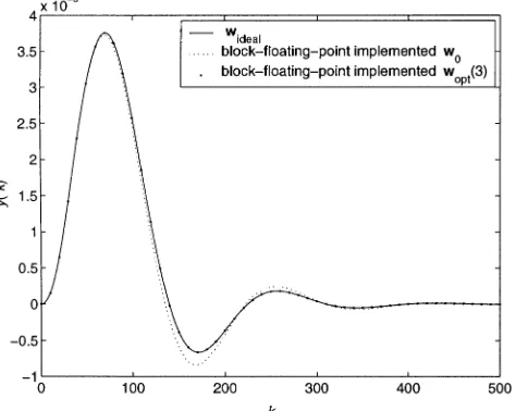
Fig. 2. Unit impulse response ofy(k) for w , 33-bit block-floating-point implementedw (two block exponent bits and 30 block mantissa bits), and 33-bit block-floating-point implementedw (3) (three block exponent bits and 29 block mantissa bits) of Example 2.

1, there are two outputsy(k) = [y₁(k)y₂(k)]T. Fig. 1 compares the unit impulse response of the first plant outputy1(k) of Example 1 for the ideal controllerw_idealwith those of the 15-bit floating-point imple-mentedw0(five exponent bits and nine mantissa bits) and the 15-bit floating-point implementedwopt(2) (five exponent bits and nine man-tissa bits). Fig. 2 compares the unit impulse response of the plant output y(k) of Example 2 for widealwith those of the 33-bit block-floating-point implementedw0(two block exponent bits and 30 block mantissa bits) and the 33-bit block-floating-point implementedwopt(3) (three block exponent bits and 29 block mantissa bits). These results clearly show that, for a chosen, the corresponding optimal realization is al-ways much better than the initial realization.

Fig. 3. Unit impulse response of y (k) for w , 22-bit fixed-point implemented w (1) (three integer bits and 18 fractional bits), 22-bit floating-point implementedw (2) (five exponent bits and 16 mantissa bits), and 22-bit block-floating-point implementedw (3) (two block exponent bits and 19 block mantissa bits) of Example 1.

Fig. 4. Unit impulse response of y(k) for w , 18-bit fixed-point implemented w (1) (eight integer bits and nine fractional bits), 18-bit floating-point implementedw (2) (four exponent bits and 13 mantissa bits), and 18-bit block-floating-point implementedw (3) (three block exponent bits and 14 block mantissa bits) of Example 2.

implementedwopt(2) (e = 4 and w = 13) and the 18-bit block-floating-point implementedwopt(3) (h = 3 and u = 14) of Ex-ample 2. It is obvious from these two figures that the response with floating-point implementedw_opt(2) is the closest to the ideal perfor-mance.

VI. CONCLUSION

We have proposed a design procedure for optimal controller realiza-tions in different representation schemes. The procedure provides de-signer with useful quantitative information regarding finite precision

computational properties, namely robustness to FWL errors and esti-mated minimum bit length for guaranteeing closed-loop stability. This allows designers to choose an optimal controller realization in an ap-propriate representation scheme to achieve the best computational ef-ficiency and closed-loop performance.

REFERENCES

[1] M. Gevers and G. Li, Parameterizations in Control, Estimation and Fil-tering Problems: Accuracy Aspects. London, U.K.: Springer-Verlag, 1993.

[2] R. S. H. Istepanian and J. F. Whidborne, Eds., Digital Controller Implementation and Fragility: A Modern Perspective. London, U.K.: Springer-Verlag, 2001.

[3] I. J. Fialho and T. T. Georgiou, “On stability and performance of sam-pled-data systems subject to wordlength constraint,” IEEE Trans. Au-tomat. Contr., vol. 39, pp. 2476–2481, Dec. 1994.

[4] G. Li, “On the structure of digital controllers with finite word length consideration,” IEEE Trans. Automat. Contr., vol. 43, pp. 689–693, May 1998.

[5] J. Wu, S. Chen, G. Li, and J. Chu, “Optimal finite-precision state-es-timate feedback controller realization of discrete-time systems,” IEEE Trans. Automat. Contr., vol. 45, pp. 1550–1554, Aug. 2000.

[6] J. Wu, S. Chen, G. Li, R. S. H. Istepanian, and J. Chu, “An improved closed-loop stability related measure for finite-precision digital controller realizations,” IEEE Trans. Automat. Contr., vol. 46, pp. 1162–1166, July 2001.

[7] J. F. Whidborne and D.-W. Gu, “Optimal finite-precision controller and filter realizations using floating-point arithmetic,” in Proc. 15th IFAC World Congr., Barcelona, Spain, July 2002, CD-ROM Paper 990. [8] R. S. H. Istepanian, J. F. Whidborne, and P. Bauer, “Stability analysis

of block floating point digital controllers,” presented at the UKACC Int. Conf. Control, Cambridge, U.K., Sept. 4–7, 2000.

[9] K. F. Man, K. S. Tang, and S. Kwong, Genetic Algorithms: Concepts and Design. London, U.K.: Springer-Verlag, 1998.

[10] S. Chen and B. L. Luk, “Adaptive simulated annealing for optimization in signal processing applications,” Signal Processing, vol. 79, no. 1, pp. 117–128, 1999.

[11] G. S. G. Beveridge and R. S. Schechter, Optimization: Theory and Prac-tice. New York: McGraw-Hill, 1970.

[12] A. J. Laub, M. T. Heath, C. C. Paige, and R. C. Ward, “Computation of system balancing transformations and other applications of simul-taneous diagonalization reduction algorithms,” IEEE Trans. Automat. Contr., vol. AC-32, pp. 115–122, Feb. 1987.

[13] J. Kautsky, N. K. Nichols, and P. Van Dooren, “Robust pole assignment in linear state feedback,” Int. J. Control, vol. 41, no. 5, pp. 1129–1155, 1985.