Word Sense Induction using Cluster Ensemble
Bichuan Zhang, Jiashen Sun
Lingjia Deng, Yun Huang, Jianri Li, Zhongwan Liu, Pujun ZuoCenter of Intelligence Science and Technology
School of Computer
Beijing University of Posts and Telecommunications, Beijing, 100876 China
Abstract
In this paper, we describe the implementation of an unsupervised learning method for Chinese word sense induction in CIPS-SIGHAN-2010 bakeoff. We present three individual clustering algorithms and the ensemble of them, and discuss in particular different approaches to represent text and select features. Our main system based on cluster ensemble achieves 79.33% in F-score, the best result of this WSI task. Our experiments also demonstrate the versatility and effectiveness of the proposed model on data sparseness problems.
1 Introduction
Word Sense Induction (WSI) is a particular task of computational linguistics which consists in automatically discovering the correct sense for each instance of a given ambiguous word (Pinto , 2007). This problem is closely related to Word Sense Disambiguation (WSD), however, in WSD the aim is to tag each ambiguous word in a text with one of the senses known as prior, whereas in WSI the aim is to induce the different senses of that word.
The object of the sense induction task of CIPS-SIGHAN-2010 was to cluster 5,000 instances of 100 different words into senses or classes. The task data consisted of the combination of the test and training data (minus the sense tags) from the Chinese lexical sample task. Each instance is a context of several sentences which contains an occurrence of a given word that serves as the target of sense induction.
The accuracy of the corpus-based algorithms for WSD is usually proportional to the amount of hand-tagged data available, but the construction of that kind of training data is often difficult for
real applications. WSI overcomes this drawback by using clustering algorithms which do not need training data in order to determine the possible sense for a given ambiguous word.
This paper describes an ensemble-based unsupervised system for induction and classification. Given a set of data to be classified, the system clusters the data by individual clusters, then operates cluster ensemble to ensure the result to be robust and accurate accordingly.
The paper is organized as follows. Section 2 gives an description of the general framework of our system. Sections 3 and 4 present in more detail the implementation of feature set and cluster algorithms used for the task, respectively. Section 5 presents the results obtained, and Section 6 draws conclusions and some interesting future work.
2 Methodology in Sense Induction Task
Sense induction is typically treated as an unsupervised clustering problem. The input to the clustering algorithm are instances of the ambiguous word with their accompanying contexts (represented by co-occurrence vectors) and the output is a grouping of these instances into classes corresponding to the induced senses. In other words, contexts that are grouped together in the same class represent a specific word sense.
In this task, an instance to be clustered is represented as a bag of tokens or characters that co–occur with the target word. To exploit the diversity of features, besides the co–occurrence matrix, we invoke the n-gram such as bi-grams that occur in the contexts. For assigning a weight for each term in each instance, a number of alternatives to tf-idf and entropy have been investigated.
Obviously, a single document has a sparse vector over the set of all terms. The performance of clustering algorithms will decline dramatically due to the problems of high dimensionality and data sparseness. Therefore it is highly desirable to reduce the feature space dimensionality. We used two techniques to deal with this problem: feature selection and feature combination.
Feature selection is a process that chooses a subset from the original feature set according to some criterion. The selected feature retains original physical meaning and provides a better understanding for the data and learning process. Depending on whether the class label information is required, feature selection can be either unsupervised or supervised. For WSI should be an unsupervised fashion, the correlation of each feature with the class label is computed by distance, information dependence, or consistency measures.
Feature combination is a process that combines multiple complementary features based on different aspects extracted at the selection step, and forms a new set of features.
The methods mentioned above are not directly targeted to clustering instances; in this paper we introduce three cluster algorithms: (a) EM algorithms (Dempster et al., 1977; McLachlan and Krishnan, 1997), (b) K-means (MacQueen, 1967), and (c) LAC (Locally Adaptive Clustering) (Domeniconi et al., 2004), and one cluster ensemble method to incorporate three results together to represent the target patterns and conduct sense clustering.
We conduct multiple experiments to assess different methods for feature selection and feature combination on real unsupervised WSI problems, and make analysis through three facets: (a) to what extent feature selection can improve the clustering quality, (b) how much width of the smallest window that contains all the co–occurrence context can be reduced without losing useful information in text clustering, and (c) what index weighting methods should be applied to sense clustering. Besides the feature exploitation, we studied in more detail the performance of cluster ensemble method.
3 Feature Extraction
3.1 Preprocessing
Each training or test instance for WSI task contains up to a few sentences as the surrounding context of the target word w, and the number of
the sense of w is provided. We assume that the
surrounding context of a target w is informative
to determine the sense of it. Therefore a stream of induction methods can be designed by exploiting the context features for WSI.
In our experiment, we consider both tokens (after word segmentation) and characters (without word segmentation) in the surrounding context of target word w as discriminative
features, and these tokens or characters can be in different sentences from instances of w. Tokens
in the list of stop words and tokens with only one character (such as punctuation symbols) are removed from the feature sets. All remaining terms are gathered to constitute the feature space of w.
Since the long dependency property, the word sense could be relying on the context far away from it. From this point, it seems that more features will bring more accurate induction, and all linguistic cues should be incorporated into the model. However, more features are involved, more serious sparseness happens. Therefore, it is important to find a sound trade-off between the scale and the representativeness of features. We use the sample data provided by the CIPS-SIGHAN as a development data to find a genetic parameter to confine the context scale. Let ω be the width of the smallest window in an instance d that contains terms near the target
word, measured in the number of words in the window. In cases where the terms in the window do not contain all of the informative terms, we can set ω to be some enormous number (ω < the length of sentence). Such proximity-weighted scoring functions are a departure from pure cosine similarity and closer to the “soft conjunctive” semantics.
Token or character is the most straightforward basic term to be used to represent an instance. For WSI, in many cases a term is a meaningful unit with little ambiguity even without considering context. In this case the bag-of-terms representation is in fact a bag-of-words, therefore N-gram model can be used to exploit such meaningful units. An n-gram is a sequence of n
consecutive characters (or tokens) in an instance. The advantages of n-grams are: they are language independent, robust against errors in instance, and they capture information about phrases. We performed experiments to show that for WSI, n-gram features perform significantly better than the flat features.
A simple approach is TF (term frequency) using the frequency of the word in the document. The schemes take into account the frequency of the word throughout all documents in the collection. A well known variant of TF measure is TF-IDF weighting which assigns the weight to word i in
document k in proportion to the number of
occurrences of the word in the document, and in inverse proportion to the number of documents in the collection for which the word occurs at least once.
*log( )
ik ik
i N
a f
n
=
Another approach is Entropy weighting, Entropy weighting is based on information theoretic ideas and is the most sophisticated weighting scheme. It has been proved more effective than word frequency weighting in text representing. In the entropy weighting scheme, the weight for word in document is given by a
i
k
ik.
1
1
log( 1.0)* 1 log( )
log( )
N
ij ij
ik ik
j i i
f f
a f
N = n n
⎛ ⎡
= + ⎜⎜ + ⎢
⎣
⎝
∑
⎞ ⎤
⎟ ⎥ ⎟ ⎦ ⎠ Re-parameterization is the process of constructing new features as combinations or transformations of the original features. We investigated Latent Semantic Indexing (LSI) method in our research and produce a term-document matrix for each target word. LSI is based on the assumption that there is some underlying or latent structure in the pattern of word usage across documents, and that statistical techniques can be used to estimate this structure. However, it is against the primitive goal of the LSI weighting that LSI performs slightly poorer compared with the TF, TF-IDF and entropy. The most likely reason may is that the feature space we construct is far from high-dimension, while feature the LSI omitted may be of help for specific sense induction.
3.2 Feature Selection
A simple features election method used here is frequency thresholding. Instance frequency is the number of instance to be clustered in which a term occurs. We compute the instance frequency for each unique term in the training corpus and remove from the feature space those terms whose instance frequency was less than some predetermined threshold (in our experiment, the threshold is 5). The basic assumption is that rare terms are either non-informative for category prediction, or not influential in global
performance. The assumption of instance frequency threshold is more straightforward that of LSI, and in either case, removal of rare terms reduces the dimensionality of the feature space. Improvement in cluster accuracy is also possible if rare terms happen to be noise terms.
Frequency threshold is the simplest technique for feature space reduction. It easily scales to sparse data, with a computational complexity approximately linear in the number of training documents. However, it is usually considered an ad hoc approach to improve efficiency, not a principled criterion for selecting predictive features. Also, frequency threshold is typically not used for aggressive term removal because of a widely received assumption in information retrieval. That is, low instance frequency terms are assumed to be relatively informative and therefore should not be removed aggressively. We will re-examine this assumption with respect to WSI tasks in experiments.
Information gain (IG) is another feature felection can be easily applied to clustering and frequently employed as a term-goodness criterion in the field of machine learning. It measures the number of bits of information obtained for cluster prediction by knowing the presence or absence of a term in an instance.
Since WSI should be conducted in an unsupervised fashion, that is, the labels are not provided, the IG method can not be directly used for WSI task. But IG can be used to find which kind of features we consider in Section 3.1 are most informative feature among all the feature set. We take the training samples as the development data to seek for the cues of most informative feature. For each unique term we compute the information gain and selecte from the feature space those terms whose information gain is more than some predetermined threshold. The computation includes the estimation of the conditional probabilities of a cluster given a term and the entropy computations in the definition.
m
i 1
IG(t) = -
∑
= p c( ) log ( )i p ci+p t( )
∑
mi 1= p c( | t) log ( | t)i p ci+p t( )
∑
mi 1= p c t( | ) log ( | )i p c tiwhere t is the token under consideration, ci is
of a feature selection method globally with respect to all clusters on average.
3.3 Feature combination
Combining all features selected by different feature set can improve the performance of a WSI system. In the selection step, we find the feature that best distinguishes the sense classes, and iteratively search additional features which in combination with other chosen features improve word sense class discrimination. This process stops once the maximal evaluation criterion is achieved.
We are trying to disply an empirical comparison of representative feature combination methods. We hold that particular cluster support specific datasets; a test with such combination of cluster algorithm and feature set may wrongly show a high accuracy rate unless a variety of clusterers are chosen and many statistically different feature sets are used. Also, as different feature selection methods have a different bias in selecting features, similar to that of different clusterers, it is not fair to use certain combinations of methods and clusterers, and try to generalize from the results that some feature selection methods are better than others without considering the clusterer.
This problem is challenging because the instances belonging to the same sense class usually have high intraclass variability. To overcome the problem of variability, one strategy is to design feature combination method which are highly invariant to the variations present within the sense classes. Invariance is an improvement, but it is clear that none of the feature combination method will have the same discriminative power for all clusterers.
For example, features based on global window might perform well when instances are shot, whereas a feature weighting method for this task should be invariant to the all the WSI corpus. Therefore it is widely accepted that, instead of using a single feature type for all target words it is better to adaptively combine a set of diverse and complementary features. In our experiment, we use several combination of features in multiple views, that is, uni-gram/bi-gram, global/window, and tfidf/entropy – in order to discriminate each combination best from all other clusters.
4 Cluster
There are two main issues in designing cluster
ensembles: (a) the design of the individual “clusterers” so that they form potentially an accurate ensemble, and (b) the way the outputs of the clusterers are combined to obtain the final partition, called the consensus function. In some ensemble design methods the two issues are merged into a single design procedure, e.g., when one clusterer is added at a time and the overall partition is updated accordingly (called the direct or greedy approach).
In this task we consider the two tasks separately, and investigate three powerful cluster methods and corresponding consensus functions.
4.1 EM algorithm
Expectation-maximization algorithm, or EM algorithm (Dempster et al., 1977; McLachlan and Krishnan, 1997) is an elegant and powerful method for finding maximum likelihood solutions for models with latent variables.
Given a joint distribution
(X, Z | )
p
θ
over observed variables X and latent variables Z,governed by parameters
θ
, the goal is to maximize the likelihood functionp
(X | )
θ
with respect toθ
.1. Choose an initial setting for the parameters
θ
old;2. E step Evaluate (Z | X, old);
p
θ
3. M step Evaluate
θ
new given by;
= argmax ( ,
)
new old
θ
θ
ϑ θ θ
where
( ,
old)
(Z|X, )
oldln (X,Z| )
z
p
p
ϑ θ θ
=
∑
θ
θ
4. Check for convergence of either the log likelihood or the parameter values. If the convergence criterion is not satisfied, then let
old new
θ
←
θ
and return to step 2.
4.2 K-means
K-means clustering (MacQueen, 1967) is a method commonly used to automatically partition a data set into k groups. It proceeds by
selecting k initial cluster centers and then
iteratively refining them as follows:
1. Each instance d is assigned to its closest
cluster center. i
2. Each cluster center C is updated to be the
mean of its constituent instances. j
using instances chosen at random from the data set. The data sets we used are composed of numeric feature, for numeric features, we use a Euclidean distance metric.
4.3 LAC
Domeniconi et al.(2004) proposed an Locally Adaptive Clustering algorithm (LAC), which discovers clusters in subspaces spanned by different combinations of dimensions via local weightings of features. Dimensions along which data are loosely correlated receive a small weight, which has the effect of elongating distances along that dimension. Features along which data are strongly correlated receive a large weight, which has the effect of constricting distances along that dimension. Thus the learned weights perform a directional local reshaping of distances which allows a better separation of clusters, and therefore the discovery of different patterns in different subspaces of the original input space.
The clustering result of LAC depends on two input parameters. The first one is common to all clustering algorithms: the number of clusters
k to be discovered in the data. The second one
(called h) controls the strength of the incentive to cluster on more features. The setting of h is
particularly difficult, since no domain knowledge for its tuning is likely to be available. Thus, it would be convenient if the clustering process automatically determined the relevant subspaces.
4.4 Cluster Ensemble
Cluster ensembles offer a solution to challenges inherent to clustering arising from its ill-posed nature. Cluster ensembles can provide robust and stable solutions by leveraging the consensus across multiple clustering results, while averaging out emergent spurious structures that arise due to the various biases to which each participating algorithm is tuned.
Kuncheva et al. (2006) has shown Cluster ensembles to be a robust and accurate alternative to single clustering runs. In the work of Kuncheva et al. (2006), 24 methods for designing cluster ensembles are compared using 24 data sets, both artificial and real. Both diversity within the ensemble and accuracy of the individual clusterers are important factors, although not straightforwardly related to the ensemble accuracy.
The consensus function aggregates the outputs of the Individual clusterers into a single partition. Many consensus functions use the consensus
matrix obtained from the adjacency matrices of the individual clusterers. Let N be the number of
objects in the data set. The adjacency matrix for clusterer
k
is an N by N matrix with entry( , ) 1
i j
=
if objects i and j are placed in the same cluster by clusterer , andk
( ,
i j
) 0
=
, otherwise. The overall consensus matrix, M, is the average of the adjacency matrices of the clusterers. Its entry gives the proportion of clusterers which put and( , )
i j
i j in the same cluster. Here the overall consensus matrix, M, can be
interpreted as similarity between the objects or the “data”. It appears that the clear winner in the consensus function “competition” is using the consensus matrix as data. Therefore, the consensus functions used in the WSI task invoke the approach whereby the consensus matrix M is used as data (features). Each object is represented by N features, i.e., the j-the feature
for object is the i
( ,
i j
)
entry of M.Then we use Group-average agglomerative clustering (GAAC) to be the consensus functions clustering the M matrix.
5 Analysis
First, we conducte an ideal case experiment on the training samples provided by CIPS-SIGHAN 2010, to see whether good terms can help sense clustering. Specifically, we applied supervised feature selection methods to choose the best feature combinations driven by performance improving on the training features. Then, we executed the word sense induction task using features under the prefered feature combinations and compare the various clustering results output by three individual cluster.
We then designe cluster ensemble method with results on three clusters, distributed as M
data consensus matrix.
5.1 Soundex for Feature
We apply feature selection and feature combination to instances in the preprocessing of K-means, EM and LAC. The effectiveness of a combination method is evaluated using the performance of the cluster algorithm on the preprocessed WSI. We use the standard definition of recall and precision as F-score (Zhao and Karypis, 2005) to evaluate the clustering result.
desired degree from the full feature set of WSI corpus.
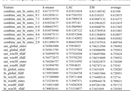
Table 2 shows The F-score figures for the different combinations of knowledge sources and learning algorithms for the training data set. The feature columns correspond to:
(i) tfidf: tf-idf weighting (ii) entro: Entropy weighting (iii) bi: bi-gram representation (iv) uni: uni-gram representation
(v) global: using all the terms in the instance
(vi) winXX: using only terms in the surrounding context, and the width of the window is the figure followed by. As shown in Table 2, the best averaged F-score for WSI (without combination) is obtained by global_entro by maintaining a very consistent result for three cluster algorithm. That is, the feature weighting method will dominate
Feature k-means LAC EM average
[image:6.595.78.513.194.495.2]combine_uni_bi_entro_8:2 0.817375775 0.819315654 0.811188742 0.81596 combine_uni_bi_entro_9:1 0.812858111 0.817265352 0.81510355 0.815075 combine_uni_bi_entro_7:3 0.805319576 0.817909374 0.819887132 0.814372 combine_uni_bi_entro_1:1 0.810324177 0.81397143 0.812962625 0.812419 combine_uni_bi_entro_6:4 0.806647971 0.815069965 0.810440791 0.811945 combine_uni_bi_entro_1:9 0.810576944 0.811287122 0.813785918 0.811883 combine_uni_bi_entro_4:6 0.810475113 0.810512846 0.811584054 0.810857 combine_uni_bi_entro_3:7 0.809265111 0.811142052 0.811340668 0.810582 combine_uni_bi_entro_2:8 0.811090379 0.804433939 0.813767918 0.809764 uni_global_entro 0.765063808 0.75954835 0.746212504 0.756942 uni_global_tfidf 0.765011785 0.757537564 0.745006996 0.755852 uni_win30_tfidf 0.764949578 0.757424304 0.744497086 0.755624 uni_win40_tfidf 0.764772672 0.755702292 0.744319609 0.754932 uni_win30_entro 0.764286757 0.755514592 0.742825875 0.754209 uni_win40_tfidf 0.763994795 0.75954835 0.742747114 0.75543 bi_global_entro 0.740026161 0.731310077 0.71651859 0.729285 bi_global_tfidf 0.739555095 0.731264758 0.716031966 0.728951 bi_win30_entro 0.737209909 0.729711844 0.714498518 0.72714 bi_win40_entro 0.715230191 0.713987571 0.699644178 0.709621 bi_win40_tfidf 0.714031488 0.710282928 0.697201196 0.707172 bi_win30_ tfidf 0.740026161 0.731310077 0.71651859 0.729285
Table 1: Feature selection for our system.
the F-score. On the other hand, we should combine uni_global_entro and bi_global_entro to improve the cluster performance:
(vii) combine: combining all two feature (uni and bi) with the at the rate of the ratio followed by.
From these figures, we found the following points. First, feature selection can improve the clustering performance when a certain terms are combined. For example, any feature combination methods can achieve about 5% improvement. Second, as can be seen from Table 1, the best performances yielded at the combination ratio of 8:2. As can be seen, when more bi-gram terms are added, the performances of combination methods drop obviously. In order to find out the reason, we compared the terms selected at
uni-gram features and top 20% features as the final clustering features.
5.2 The cluster ensembles
As described in Section 5.1, we use two language models (uni-gram and bi-gram), 4 types of the context window (20, 30, 40 and global) and 2 feature weighting methods (tf-idf and entropy), also, 10 combined feature set and 3 cluster algorithm is introduced; in the other word, we have at least 78 result, that is 78 consensus matrix interpreted as “data” to be aggregated. Thus we can evaluate the statistical significance of the difference among any ensemble methods on any cluster result set.
To compare all ensemble methods, we group the result sets (out of 78) into different feature representation scheme. Significant difference for a given feature representation methods, the ensemble result is observed to check weather cluster ensembles can be more accurate than single feature set and to find out which method appears to be the best choice for the WSI task.
Table 2 shows the ensembles examined in our experiment. The feature columns correspond to different group of result set, for example, bi_tfidf indicates bi-gram model and tf-idf feature weighting methods are selected, all the 3 cluster results on win20, win30, win 40 and global feature sets (12 consensus matrix) are aggregated; complex_entro indicates that all the feature representation methods selecting entropy weighting are chosen.
Results show that the best performance is the group in which all the outputs of all the clusterers are combined (the top row in Table 2).
Feature F1-score Scale
complex 0.827566232 78
[image:7.595.303.531.468.535.2]complex_entro 0.823006644 24 complex_nocomb 0.822970703 48 complex_global 0.821960768 12 uni_complex 0.821931155 24 uni_ entro 0.821931155 15 uni_global 0.821817211 6 complex_combine 0.819456935 30 uni_ tfidf 0.811631894 12 complex_tfidf 0.806807226 24 complex_entro 0.806063712 24 bi_complex 0.801211134 24 bi_entro 0.794939656 12 bi_global 0.788673134 6 bi_tfidf 0.788170215 12
Table 2: Ensemble designs sorted by the total index of performance
5.3 CIPS-SIGHAN WSI Performance
The goal of this task is to promote the exchange of ideas among participants and improve the performance of Chinese WSI systems. The input consists of 100 target words, each target word having a set of contexts where the word appears. The goal is to automatically induce the senses each word has, and cluster the contexts accordingly. The evaluation measures provided is F-Score measure. In order to improve the overall performance, we used two techniques: feature combination and Cluster Ensemble.
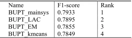
We chose combinomg global size of window, entropy weighting, uni-garm and bi-gram at the ratio of 8:2 as the final feature extraction method. Three powerful cluster algorithms, EM, K-means and LAC recieve these features as input, and in our main system all the outputs of all the clusterers are combined to process cluster ensemble. In Table 3 we show four results obtained by three individual clusters and one ensemble of them.
Our main system has outperformed the other systems achieving 79.33%. Performance for LAC is 78.95%, 0.4% lower the best system. For EM our F-sore is 78.55%, which is around 0.8% lower than the best system, the similar result ia also observed for K-means. The results of our system are ranked in the top 4 place and obviously better the other systems.
Name F1-score Rank
BUPT_mainsys 0.7933 1
BUPT_LAC 0.7895 2
BUPT_EM 0.7855 3
BUPT_kmeans 0.7849 4
Table 3: Evaluation (F-score performance)
6
ConclusionsIn this paper, we described the implementation of our systems that participated in word sense induction task at CIPS-SIGHAN-2010 bakeoff. Our ensemble model achieved 79.33% in F-score, 78.95% for LAC, 78.55% for EM and 78.49% for K-means. The result proved that our system had the ability to fully exploit the informative feature in senses and the ensemble clusters enhance this advantage.
[image:7.595.70.290.539.745.2]Acknowledgement
This research has been partially supported by the National Science Foundation of China (NO. NSFC90920006). We also thank Xiaojie Wang, Caixia Yuan and Huixing Jiang for useful discussion of this work.
References
D. Pinto, P. Rosso, and H. Jim´enez-Salazar. UPV-SI: Word sense induction using self term expansion. In Proc. of the 4th International Workshop on Semantic Evaluations - SemEval 2007. Association for Computational Linguistics, 2007. pp. 430-433. Yiming Yang and Jan O. Pedersen. A Comparative
Study on Feature Selection in Text Categorization. In Proceedings of the 14th International Conference on Machine Learning (ICML), 1997. pp. 412-420.
Salton, Gerard, and Chris Buckley. 1987. Term weighting approaches in automatic text retrieval. Technical report, Cornell University, Ithaca, NY, USA.
S. Dumais, Improving the retrieval of information from external sources, Behavior Research Methods, Instruments, & Computers, 1991, 23:229-236. M. W. Berry, S. T. Dumais, and G. W. O'Brien, Using
linear algebra for intelligent information retrieval, SIAM Rev., 1995, 37:573-595
MacQueen, J. B. (1967). Some methods for classification and analysis of multivariate observations. Proceedings of the Fifth Symposium on Math, Statistics, and Probability, Berkeley, CA: University of California Press. pp. 281-297.
Dempster,A.P., Laird,N.M and Rubin,D.B. (1977) Maximum likelihood from incomplete data via the EM algorithm. J. Roy. Statist. Soc. B, 39, 1-38. MCLACHLAN, G., AND KRISHNAN, T. 1997. The
EM algorithm and extensions. Wiley series in probability and statistics. JohnWiley & Sons. Y. Zhao and G. Karypis. 2002. Evaluation of
hierarchical clustering algorithms for document datasets. In Proceedings of the 11th Conference of Information and Knowledge Management (CIKM), pp. 515-524.
K. Aas and L. Eikvil. Text categorisation: A survey. Technical Report 941, Norwegian Computing Center, June 1999.
C. Domeniconi, D. Papadopoulos, D. Gunopulos, and S. Ma. Subspace clustering of high dimensional data. SIAM International Conference on Data Mining, 2004.