Accurate Numerical Steady State and Transient One Dimensional Solutions of Semiconductor Devices

Copyright ~ by

ACCURATE NUMERICAL STEADY-STATE AND TRANSIENT ONE-DIMENSIONAL SOLUTIONS OF SEMICONDUCTOR DEVICES

Thesis by

Andrea De Mari

In Partial Fulfillment of the Requirements

For the Degree of Doctor of Philosophy

California Institute of Technology Pasadena, California

1968

i i

ACKNOWLEDGEMENTS

I am very much indebted and grateful to Professor R. D. Middlebrook for his help and guidance. This work was in part supported by the

U.S. Navy through Contracts

N123(60530)516o8A, N123(60530)54694A,

N00123-67-C-1187,

and partially conducted with the assistance of a

iii ABSTRACT

Numerical iterative methods of solution of the one-dimensional basic two-carrier trans~ort equations describing the behavior of semi-conductor junctions under bothsteady-state and transient conditions are presented. The methods are of a very general character: none of the conventional assumptions and restrictions are introduced, and free-dom is available in the choice of the doping profile, generation-recom-bination law, mobility dependencies, injection level, and boundary

conditions applied solely at the external contacts. For a specified arbitrary input signal of either current or voltage (as a function of time) the soiution yields termina1 properties and al.1 the quantities of interest in the interior of the device, such as carrier densities, electric field, electrostatic potential, particle and displacement currents, as 'fLLnctians 0£ ~osition (and time).

The work is divided into two parts. In Part I a numerical method of solution of the steady-state problem, already available in the literature, is improved and extended, and is applied to a two-contact and a three-contact device. The analytical formuJation of the original method is shown to be unsuitable for generating a sound numerical

iv

first-order results of the terminal properties for particular bias conditions. Results for an N-P-N transistor are also reported and the inadequacy of the one-dimensional model discussed,

The time-dependent analysis of the problem is presented in Part II.

The fundamental equations are rearranged to an equivalent set of three non-linear partial differential equations more suitable for numerical methods. A highJ.y non-uniform two-dimensionaJ. mesh, subject to

maintenance of constant truncation errors in both spatial a~d time

domains of certain pointwise operations, is chosen for the discretization of the problem, in view of the variation of most quantities over extreme ranges within short regions. Consequently an implicit discretization scheme is selected for the second-order partial differential equations of' the parabolic type in order to avoid restrictions on the mesh siz~,

without endangering numerical stability. An iterative procedure is

necessary at each instant of time to cope with the several non-linearities of the problem and to achieve consistency between the internal distribu-tions and the generating equadistribu-tions. This procedure is easily general-ized to incorporate equations pertinent to networks of passive elements and ideal generators connected to the semiconductor device. Results for a particular single-junction structure under typical time-dependent excitations of external current and termina1 voltage, and for an N-P diode interacting with an external resistor under switching conditions, are reported and discussed in detail,

v

difficul.~ies of the problem, such as the small differences between nearly equal numbers, the variation of most quantities over extremely wide ranges in short regions, and the stability conditions related to the discretization of partial differential equations of the parabolic

vi

TABLE OF CONTENTS

INTRODUCTION l

PART I

CHAPTER I OUTLINE OF THE METHOD FOR THE SOLUTION OF THE DIRECT

PROBLEM (VA ... J) FOR A TWO CONTACT DEVICE 8

1.1. Physical and mathematical model 1.1.l.

1.1.2.

1.1.3.

}'undrunental equations

Normalization of the fundamental equations Boundary conditions

l.2. Derivation of the reduced set or equations

1.3. Iterative procedure of solution l.3.l. Two ~pBcl~l c~~B~

1.4.

Conclusion

CHAPTER II IMPROVED ANALYTICAL FORMULl\.TION AND NUMERICAL

TECH-8 8

l4

17

l9 22 25

27

NIQUES 29

2.l. Generalities

2.2. Improved analytical formulation

30

3l 2.2.1, Small differences between nearly equal numbers 3l 2.2.2. Extension to high reverse bias conditions

35

2.3.

Numerical techniques

2.3.1.

2.3.2.

2.3.3.

Automatically adjustable non-uniform step distribution

Numerical integration and differentiation Numerical solution of Poisson's equation 2.4. Computer program for a special case

2.5.

Conclusion

4l

4l

62

65

72

72 CHAPTER III 'IWO SIMPLE: APPLICATIONS OF THE BASIC DIRECT PROORAM 75

3.1.

Generalities

3.2.

Computation of the total incremental capacitance

3 ,3. A solution for the reverse problem (J .... VA)

3.3;1.

Description of the method

3,3.2.

Results

3.4.

Conclusion

vii

CHAPI'ER IV EXTENSION OF THE METHOD TO THE SOLUTION OF THE

TRANSISTOR 84

4.1. Mathematical model and boundary conditions 84

4. 2. Analytical formulation 88

4.3.

Iterative procedure for the direct and reverse problem 92

4.4. Conclusion

95

CHAPTER V ON THE ACCURACY OF THE NUMERICAL RESULTS 5.1. Generalities

5.2. Sources of error

5.2.1. Discretization error 5.2.2. Numerical error

5.2.3. Physical model discretization error 5.3. Influence and control of the errors

5.3.1. Discretization error

5.3.2.

Numerical error

5.3.3. Physical model discretization error

5.4. Testing criteria of the accuracy of the results

5.5.

Conclusion

CHAPTER VI RESULTS 6.1. Generalities

97

97

98

98

99

99

99

99

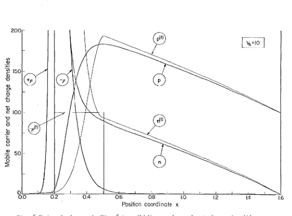
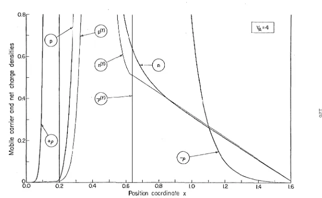
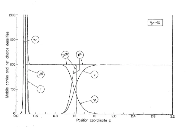
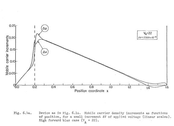
102 104 104 10'7 109 109

6. 2. A two-contact device: the N-P diode 110 6.2.l. External contacts of the ohmic type 111 6.2.2. A finite value o~ surface recombination velocity

at one external contact 141

6.3. A three-contact device: the N-P-N transistor

148

6.4. Conclusion

177

PART II

CHAPTER VII ANALYTICAL FORMUIATION OF TEE CURRENT-DRIVEN

TRANSIENT PROBIEM FOR A '.IWO-CONTACT DEVICE 7.l. Generalities

7.2.

Physical and mathematical model

7.2.1. 7.2.2.

Normalized fundamental equations Boundary and initial conditions

7.3.

Derivation of the reduced set of equations

viii 7.4. Iterative method of solution 7.5. Conclusion

CHAPTER VIII DISCRETIZATION OF T.:-IE ANA.LYTICAL FORMUIATION FOR

188 190

THE CURRENT-DRIVEN '.i:'RANSIENT 193

8.l. Selection of the discretization scheme 193

8.2. Discretization by implicit schemes

197

8.2.1. Generalized pure implicit scheme l98 8.2.2. Generalized Crank-Nicholson scheme 2CJ7 8.3. Detailed iterative procedure of solution 211 8.4. Automatically adjustable non-uni~orzn discretization

mesh 218

8.5. Conclusion

CHAPTER DC VOLTAGE-DRIVEN TRANSIENT 9.1.

9.2. 9.3. 9.4.

9.5. CHAPTER X

Generalities

Voltage-driven transient: outline of the method A ~om:pa.tible steady-stat£=~ solution

~ime-dependent solutions for the combination of an active device with a network of passive circuit elements

Conclusion

ON THE ACCURACY OF THE TRANSIENT SOLUTIONS

223 225 225 227 234 237 241 242

10.l. Generalities 242

10.2. Discretization error in the time domain 243 10.3. Numerical error and its growth in the time domain 246

10.3.1. Iteration error 247

10.3.2. Inaccuracy of_ the initial conditions 250 l0.3.3. Tolcr~ncc on the opccificd excitation in the

voltage-driven transient 251

10.4. Conclusion CHAPTER XI RESULTS

252 253

11.l •. Generalities 253

11. 2. The N-P diode driven by ideal current and voltage sources

11.2.1. Excitation: 11.2.2. Excitation:

a low current step a high current step

ix

11.2.3. Excitation: a spike of current 11.2.4. Excitation:· a low voltage step

.Ll,j. The interaction 01· the N-P diode and an external

281

287

resistor under switching conditions

298

· 11.4. Conclusion 313

CHAPTER XII CONCLUSIONS 314

APPENDIX A SOME RESULTS OF THE CONVENTIONAL FIRST-ORDER

THEORY FOR THE N-P JUNCTION IN STEADY-STATE 320

APPENDIX B NUMERICAL INTEGRATION AND DIFFERENTIATION

APPENDIX C CQ\1PUTER PROORAM FOR THE DIRECT STEADY-STATE :PR OH IBM

APPENDIX D COMPUTER PRCGRAM FOR 'lliE CALCULATION OF THE

TOTAL INCREMENTAL CAPACITANC'E

APPENDIX E COMPUTER PROGRAM FOR THE REVERSE STEADY-STATE

PROBLEM

APPEND:lX F ON TEE NUMERICAL SOLUTION OF SECOND ORDER PARTIAL

DIFF'ERENTI!l.L EQ,UATIONS OF TEE PARADOLIC TYPE

APPENDIX G COMPUTER PROORAM FOR THE TRANSIENT DIRECT AND REVERSE PROBLEMS

LIST OF PRINCIPAL SYMBOLS

l

INTRODUCTION

B~oic concepto in the theory of the

r-N

junction were first pre-sented in Shockley's fundamental paper [l] with an approximate solu-tion for the low-level injecsolu-tion case, and many authors presented in the following years extensions) ('01"l"P.r.tionfl ana ref'inement.R in the

search for a generalized solution to the problem. A comprehensive bibliography is given by Moll [2], Pritchard [3], and Matz [4], and more recent considerations have been presented by Middlebrook [5], Van Vliet

[6],

and Sah [7], Only partial success has so far been achieved; this is due mainly to serious difficulties in the analytical solution of the pertinent set of equations that describe mathematically even the simplest physical model.

In order to achieve analyticci.l .n:i::iulLs in closed form, a number o~

asswnptions in the model and of approximations in the set of equations has been consistently introduced; several "first-order" results, valid

in certain ranges of the relevant quantities and for a limited number

of specialized structures, have been obtained. Some of these asswnp-tions for the one-dimensional model (to which attention will be

limited in this paper) are the follO'Wing:

(a) separation of the structure into regions with shar~ boundaries, either fully depleted of mobile carriers, or space-charge neutral; (b) postulation of explicit boundary conditions on the relevant

quan-tities in the interior of the device, at the interfaces between the depleted and neutral regions o!' assumption (a); limited choice of boundary conditions at the external contacts;

2

step and linear distributions) and to particular quantitative values (either symmetric or highly asymmetric impurity distribu-tions);

(d) simplification of the dependence of the carrier mobilities upon electric field, doping and scattering phenomena;

( e) limitation of carrier recombination laws to the low-level linear case.

The most unsatisfactory of the above assumptions is certainly the first, which is definitely in error at high injection levels, highly questionable near equilibrium, and probably only slightly inaccurate in high reverse bias cases.

Numerical methods, with the aid of high-speed digital computers, represent an alternative approach to the problem, the final aim being the achievement of an 11

exact11

solution of the most general character with none of the conventional assumptions. This also allows comparison with the classical first-order theory results so that the goodness (or poorness) of the numerous conventional assumptions may be judged.

Serious difficulties are also present in a numerical

investiga-tion, and have prevented most of the cu.rrent1y available numerical

solutions from having the general character desired. These difficul-ties arise already in the much simpler metal-semiconductor junction . case treated by Macdonald [8], and are rPspnmdhlP fo'Y' thP :::i.ccepta.nce . of some of the conventional assumptions in the P-N junction case,

3

numerical, solutio~ for the abrupt P-N junction in equilibrium in steady-state; van der Maesen [lG], Lieb et al. [l3], Kano and Reich

[14], and Chang [15] restrict the analysis to the injection region only in the charge-neutrality approximation with the low-level

recom-bination la.w for the case of an asymmetric abrupt junction, Fulkerson

and Nussbaum

[16]

and Sanchez

[17]

present a complete steady-state solution, again for the asymmetric abrupt case (with ohmic contacts, constant rr.obilities~ uniform doping); their method implies, though? the reduction of the two-boundary problem to an initial-value problem very much sensitive, for the case under consideration, to the several required guesses of slopes at the boundaries. This guesswork is likely to become critical in most instances, In addition the method described in Her. l6 is based upon the separation of the interior of the device into several regions and the iterative solution of various sets of approximate equatio~s, specialized for each region, matched

*

by boundary conditions at the interfaces.

The only comprehensive and general numerical procedure for the steady-state problem is presented by Gummel [18], and is applied to the solution of the transistor. The method allows for arbitrary impurity distribution, recombination law, mobility dependencies, injection level, and boundary conditions. Hypothetical regions in the interior of the device are not assumed, and the problem is tackled exclusively with the postulation of boundary conditions at the external

4

contacts for a set of basic equations valid throughout the whole interior. Although Gummel's iterative scheme is of a very general character, its analytical formulation is unsuitable for generating a sound numerical algorithm sufficiently accurate and valid for high reverse-bias conditions,

It is the purpose of the present work to present an improved and extended analytical. r·ormulation 01· Gummel' s original steady-state scheme, to present a numerical method of solution of the P-N junction under arbitrary transient conditions, to expose the difficulties of both fundamental and practical nature arising in the numerical analy-sis of the problems, and to illustrate results for particular

structures under both steady-state and transient conditions.

The presenta~ion is divided into two parts: the first is

re-stricted to the steady-state analysis and illustrates solutions obtained with the improved formulation based on Gunnnel's original iterative scheme; the second is mostly concerned with the analysis of the problem in transient conditions.

In Part I, Chapter I describes the physical model adopted for a two-contact device, the fundamental equations and boundary conditions that determine mathematically the steady-state problem, an alternative derivation of Gummel's relations featuring a more convenient choice of unknowns, and the overall iterative scheme for the "direct problem"

5

numerical techniques. Chapter III presents two applications of the basic program for the direct problem: the computation of the total

incremental capacitance of the device as obtained by two successive steady-state solutions, and a method of solution of the 11

reverse11 problem (the total current is specified), Chapter IV extends the

steady-state solution to the transistor, on the basis of Gumrnel's general lines, discusses the inadequacy of the one-dimensional model, and analyzes the effects of an alternative boundary condition for the base contact. Chapter V discusses the various sources of errors and the accuracy of the final results, tested with several sets of rela-tions, derived from the fundamental equations and suitable to expose discretization and numerical errors. Chapter VI presents steady-state results for a few special structures: terminal properties and quanti~ ties in the interior of the device are illustrated for an abru~t N-P diode and N-P-N transistor; 1

'exact" and approximate conventional

"first-order" results are compared and discrepa.ncico a.re exposed,

In Part II, Chapter VII presents an analytical formulation suitable for the achievement of numerical transient solutions for excitations of external current for a two-contact device; boundary and initial conditions are chosen. The problem of the selection of sound discretization schemes, featuring numerical stability, is

analyzed in Chapter VIII; discretized formulations are given in detail for two implicit schemes; the overall iterative procedure of solution is illustrated and a simple method for an automatic time step selec~

6

to achieve steady-state solutions is described; the time-dependent algorithm for the analysi::i of ar1 l::iolaLeu U.ev lee LI.riven uy iU.t!al generators is extended to incorporate a general network of circuit elements. Chapter X completes the discussion, initiated in Chapter V, of the overall accuracy of the results; the various contributions to the discretization and numerical errors in the time domain are identi-fied, and techni~ues to estimate and control the accuracy of the results are dPSr.l"ih<"d. As an example of numerical calculations, time-dependent solutions are illustrated in Chapter XI for a particular structure of an N-P diode under various excitations of current and voltage, and for the combination of an N-P diode and an ext~rnal resis-tor under switching from a forward to a reverse bias condition. The potential of the basic tool developed throughout the present investiga-. tion is underlined in Chapter XII; some of the several immediate

applications for the analysis of devices under more general conditions and the possibilities of extensions to more complex situations are briefly discussed,

7

PART I

8

CHAPTER ::i:

OUTLINE OF THE METHOD FOR THE SOLUTION OF THE DIRECT PROBLEM

j,yA __, J) FOR, A '.IWO CONTACT DEVICE

In this Chapter the physical model and corresponding fundamental two-carrier trans:port equations describing t.he 'hRhR.vior of semiconduc-tor junction devices are presented, then specialized and normalized for the one-dimensional steady-state case. Boundary conditions of a very general character for a two-contact device, are given to complete the mathematical description of the problem. The basic equations are then rearranged to an equivaient reduced set, more appropriate to an iterative type of procedure. Only the 11

direct11

problem (the applied voltage is specified, the total current unknown) is considered; the analysis of the 11_reverse11

problem (the total current is specified, the terminal voltage unknown) is postponed to a later chapter, Schematic block diagrams illustrate the procedure in the general and particular cases.

J..l. Physical and mathematical mod.el. 1.1.1. Fundamental equations,

The following assumptions are introduced:

(~) non-degenerate conditionc (for validity of the Boltzmann

statistics)

(b) constant temperature

(c) time-inde:pendent impurity distribution (d) full ionization of the impurities

9

by quantum mechanics. The conventional stage of approximation (see, for example, Moll [19] pp. 62-67) of the Boltzmann equation treats

electron and hole currents as a sum of a diffusion com~onent propor-tional to the carrier density gradient and a drift component repre-senting Oh.~'s law. Such a simplified form of the current flow equa-tions, together with Poisson's equation and the continuity equations for the mobile carrier~ are here taken as the mathematical description of the behavior of the device. Generation-recombination processes are assumed to be satisfactorily described by an additive expression

solely in the continuity equations for electron and hole densities. For the present purposes this expression is permitted to assume the most general form in terms of the quantities of interest, and will be left unspecified,

Although more general and complete formulations of the problem may be devised, solutions of the simplified set of equations, present-ed below, will be here referi·ed. to as "exac.;t" suluLluu1::>,

Maxwell's equations

(l.l)

'ii'. j (~, t) = O ( 1. la)

*

show the solenoidal character of the total current density j

10

exTiressed as sum of the electron and hole Tiarticle currents J'

.I:' .t' n'

and the displacement current in terms of the electrostatic potential '¥ and the dielectric constant e. The current flew equations for electrons and holes:

expre::>s the eJ.eeLron arnl l:wJ.e currents as sums of" their dr1f"t and

(1.2)

(1.3)

diffusion components, in terms of the electron charge -e, electron and hole concentrations n,

constants D , _n

Poisson's equation

p, mobilities and diffusion

(1.4)

with N(£) =ND(£) - NA(£) relates the electrostatic potential to the net spatial electric charge in terms of the mobile carrier densities and the fixed net impurity atom concentration N, which is the differ-ence between the donor and acceptor contributions ND' NA.

The continuity equations for electrons and holes

( J.. 5)

l

11

state the equality between the time variation of the carrier concen-trations in a certain region and the flow out of such a region sub-tracted from the internal net generation-recombination term described by

u.

It is of interest to observe that only six of the above equations

are independent, Equations (l.la), (1.4), (1.5) and (1.6) are related: any one of these may be obtained from the remaining three (and the

know1ene;e of' N(;i;:,) if' Poi.srnon 1 _{R eq11ati on :i.s omitted).}

If E(£_,t) is the electric field, k the Boltzmann constant, T the absolute temperature, Vt ~ kT/e the thermal voltage, then the following subsidiary relations are valid:

The one-dimensional structure of Fig. 1,1 is considered, in which

x rcprcacnto the pooition coordinate, O and L the external

con-tacts, and M the metallurgical interface between the N-material and P-material. The fundamental equations, specialized for the one-dimen-sional steady-state ca.seJ assume the simriler forms:

j = j (x) + j (x)

n P

dj

12

@

_®

N(x)

N

(x)

o-~~-<>--~~~~~~~~~~~-6----'~

0

M

L

X

x =position coordinate

13

j

(x)

= -

eµ (x) n(x) d£(x)

+

eD (x) ddn(x)

n n x n x

j

(x)

= -

eµ (x) p(x)

d~x)

- eD (x)

d~(x)

p p p dx

d 2

$(x)

=

~

[n(x) - p(x) - N(x)]

dx2 c:

=

eU(x)

dj (x)

__.Po--

= -

eu(x)

dx

with the subsidiary relations:

cpn(x)

~

'f(x) - V ln n(x)

t nI

a(x)

= eµ n(x) + eµ p(x)

n P

D (x) _p

=

µ _p (x) Vt

(1.8)

(1.9)

( 1. .1.0)

(1.11)

(1.12)

(l.13)

(1.14)

(1.15)

where nI is the intrinsic carrier concentration and cr(x) is the con-ductivity 0£ the material..

Equations (l,13) and (1.14) may be taken as definitions of the electron and hole quasi Fermi levels cpn'

Shockley [l].

~ introduced originally by

1.1. ;; . Normalization of the fundamental equat ionG.

It is very convenient a:b this stage tu express the relevant

~uantities in dimensionless form; the set of normalization constants is chosen with the criterion of achieving the highest simplification in the relations of interest. The list of normalization factors is given in Table 1.1.

The

signs of jn and jp were originally cnosen positive in the positive x direction (Eqs,(1.8) and (1.9)); in order to obtain posi-tive currents in the forward bias case for· the structure under consid-eration, a negative normalization factor is chosen for the current. Normalized electron, hole and total current densities will then be indicated by J _n (x), J (x),

p J. Hole and electron diffusion constants

are normalized in a symmetric fashion with the introduction of an arbitrary diffusion constant D .

o' for convenience in the normalized

context, the following dimensionless quantities will be used

y (x)

n D /D o n (x)

With the exception of the above, symbols adopted for the

unnormalized q_\:8.ntities will also be used for the normalized ones. For the remainder of this work, all symbols will con$istently refer to normalized quantitiP.R, nnleRR otherwise indicated.

The fundamental equations may be written in normalized terms as:

position coordinate time coordinate

electrostatic potential quasi-Fermi levels

applied (or terminal) voltage diffusion (or barrier) potential electric field

carrier densities

net impurity,- donor, and acceptor de·nsities

total, electron, and hole current densities

generation-recombination rate carrier diff'usion constants carrier mobilities

conductivity

capacitance/unit area

NOm'1.h _3.UArTTITY

-x t ~

c.pn' cpp

VA

vd

E

n, p

N, NE' NA

J, J ' J n P

u

-l -l

Yn, Yp

-1 -l

Yn' yp cr

c

symbol I numerical value

1JJ

~ v:v~-/enI

r£!n

0 Vt Vt Vt Vt

vt/1n

nI

nI

- eD₀n₁

/1n

Don1/1JJ2

Do

Do/Vt

en~

₀

/Vt

c/1tJ

9.56685 x

lo-

5 cm

9.15246 x 10-9 sec

0.025875 volt II

II

fl

270.465 volt/cm

2 .5 x 1013 cm-3 ti

::>

- ~.0418649 am~ere/cm~

21 -3 -1 2.73151 x 10 cm sec

2

l cm /sec

38.6473 cm2/volt-sec 1.54789 x

lo-

4(n cm)-l

1.48084 x 10-S farad/cm2 Table 1.1. List of normalization factors for the quantities of interEst.

[image:25.796.73.707.74.525.2]

dJ - 0

dx

-16

J _p (x) _ _{. - y} 1 _(x) [ ( ) _{P x}

d~(x)

_{dx · +} dp(x)J _dx p

dJ (x)

_dx_n_ = - U(x)

dJ (x)

-dx-=-~- =

u (

x)

with the subsidiary relations

,

~ (x) = *(x) - 1n

n(x)

n

~ _p

(x)

=

*(x)

+ 1n

p(x)

cr(x) _ n(x)

+

p(x)

- yn(x)

yp(x)

( l .J..6a.)

(l.J:r)

(1.18)

(l.19)

(l.20)

(l.21)

(1.22)

(l.23)

(1.24)

(l.25)

17

Equations (1.16) and (1.17) to (l.21) represent a set of six independ-ent equations in the six unknowns n(x), p(x), v(x), Jn(x), Jp(x),

J. Equation (l.16a) follows directly from Eqs.(1.16), (l.20), (1.21) and will be considered as the dependent equation of the set.

1.1.3. Boundary conditio~s.

It is apparent fro~ the nature of the fundamental set of ordinary differential equations that six conditions at the boundaries are

necessary. Tbese are chosen as the carrier concentrations

n(o), p(o), n(L), p(L)

and the electrostatic potential

at the external contacts 0 · and L. Either of the boundary conditions

on the electrostatic potential ma.y be taken as a reference value, the

other being directly related to the externally applied voltage VA and the diffusion potential Vd:

. ( 1. 27)

18

(1.28)

p(L)

= f

1

[J

(L),

J

(L)]

P n P

The above relations assume the simplest form for contacts of the ohmic type, defined by:

n(O)

=

nN n(L)

= np

(1. 29)

p(O)

=

PN

p(L)

= Pp

where ~ and pN (np and Pp) are the electron and hole e~uili­

brium densities at the external contact of the N-material (P-material) respectively. An equivalent definition requires charge neutrality at· . the contacts

n(O) - p(O) - N(O)

=

0

(l.30)

n(L) - p(L) - N(L)

=

0

and coincidence of the quasi-Fermi' levels at the contacts

rn _Tn (L)

= ({)

_p (L)

}

19

With the aid of Eqs. (1.30), (1.31), (1.24) and (l,25) the carrier danl:lll.,.Y uuw1U.1:L.r·y V1;;LJ..ues ct.re .re1;;Lcllly uul..C:L.l.uecl, for l.,hil:l spet:.ll:l.l case,

in terms of the doping concentrations:

f

R(of 1

Nto'

n(O) = ~ ~ ₂

J

+ + ~ [N(O) > O]

(1.32)

n(L) = ~

=

l/Pp

p(L)

=

Pp

=

[N~L)J

2 + 1 -

N~L)

[N(L) s O]

J.. 2. Derivation o:t" the reduced set of equations.

It is convenient to rearrange Eqs.(1.17) to (1.21) in a form more appropriate for numerical methods.

Equations (1.17) and (l.18), rewritten as

d~x)

+ E(x) n(x)

=

- y _n (x) J _n (x)

d~(x)

- E(x) p(x)

=

y

(x) JP(x) ,

a.x p

may be treated as two independent first-order linear differential

equations in the unknowns n(x) and p(x), respectively, if the other quantities are considered as non-constant coefficients, Analytic

solutions are straightforward:

jE(x)dx[f .

20

. -J::J(x)dx

J

p(x) = e y (x) J (:x:) e dx + C

p p p

c

and C being integration constants. A more definite form is

n P

obtained if x and L are taken as limits of integrations, and if

c

and C are expressed in terms of the boundary conditions at the

n P

point L:

n(x) = eV(x)Qyn(x') Jn(x') .-w(x') ax•+ n(L) .-V(L)

J

p(x)

=

.-V(x)

[-1

yp(x') JP(x') et(x•) ax• + p(L) eV(L)

J

(l.33)

(l.34)

The current densities Jn' JP may be expressed in terms of U(x)

and *(x).

Integration of

Eqs.(1.20)

and

(l.21)

yields:

x

Jn(x) =

-1

U(x') dx' + Kn 0

x

Jp(x) =

1

U(x') dx' + KP

0

(l.35)

(1,36)

The constants of integration _{K '}

n K p are readily obtained by inserting

Eqs.(1.35), (1~36) respectively into Eqs.(l.33), (l.34) evaluated at x

=

0:

n( o) = e V(O)

U

yn (x)e -jl(x) (

-1

U(x' )dx'. + Kn) dx + n(L)e-V(L)

J

(l.37)

21

The expressions for Kn and K _p found from Eqs. (1.37), (l.38) can be inserted into Eqs.(1.35), (1.36) to give the final results for the current densities in terms of the potential distributions:

J (x) n

x

=

-1

u(x1

)dx1 + 0

x JP(x)

=

Ju(x1

)d.x1 +

0 _(l.40)

Gumrnel's relations are essentially contained in the above and have been here derived directly from the basic equations, rather than through the introduction of' a set of identities [l8].

The five basic equations (1.17) to (l.21) have been rearranged to a reduced set of three equations [Eq. (1.19) and Eqs. (1.33), (1.34) com-· bined with relations (l,39), (l.40)] with the boundary conditions (l.27) ..

(l,28). In this new formulation of the problem the electrostatic potential

t,

the electron density n and the hole density p are chosen as the independent quantities and represent the unknowns of the reduced set of equations.

If generation-recombination processes are neglected [U(x)

=

O], Eqs.(1.39) and (l.40) assume the simpler forms:

p(L) e•(L) - p(o) e•(o)

~y

(x) ew(x) dx

0 p

(l.42)

which clearly shows the solenoidal character of each current through-out the interior of the device in this special case.

1.3. Iterative procedure of solution.

An iterative procedure may now be emp1oyed to cope with the

several nonlinearities of the problem, For this purpose it is conveni~

ent to rearrange Poisson's Eq.(1,19) in a more appropriate form, in terms of a quantity with zero boundary values, The correction

6(j+l)(x) between the electrostatic potential distributions obtained by consecutive iterations (j+l) and (j) is introduced, and defined as:

j = 1, 2, 3, •••

where

~(j)(x)

and *(j+i)(x) are the potential distributions

at

the completion of the (j)th and (j+l)th iterations respectively. It is readily verified that:

j

=

1, 2, 3, ••• (l.43)

a.s desired. Poisson';:;, Eg_.(l..l.9) may bi::: wrll..l..en, in Lerms o:f the

g_uasi-Fermi levels (l.24), (l.25), for the (j+l)th iteration as:

d2W(j+~)(x)

=

.~(j+l)(x)

-

~~j)(x)

-

.~~j)(x)

- v(j+l)(x) -

N(~l

or

d26(j+l)(x)

•")

a.x"'

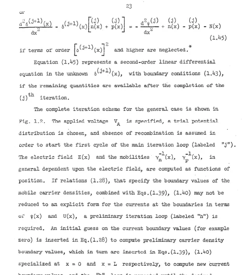
23

d2¥(j) (j) (j)

___... __ + n(x) - p(x) - N(x)

dx2

·X.

and higher are neglected.

(1.45)

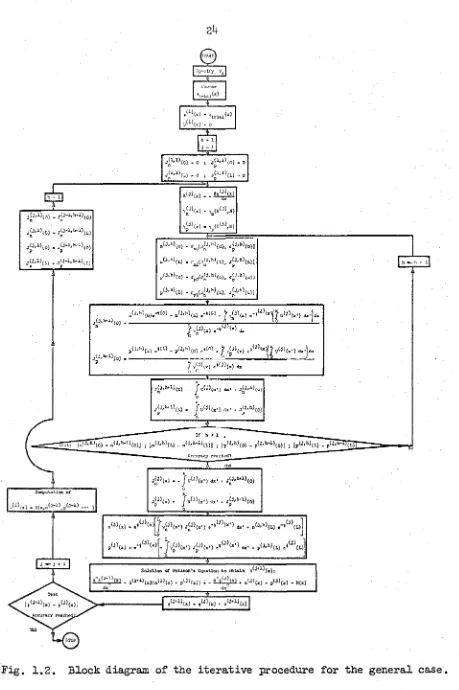
Equation

(1.45)

represents a second-order linear differential equation in the unknown 6(j+l)(x), with boundary conditions (1.43), if the remaining quantities are available after the completion of the (j)th iteration.

The complete iteration scheme for the general case is shown in Fig. l.?.. The applied voltage VA is s:pe~if'ied, a t'Y'i::tl potenti::i.l distribution is chosen, and absence of recombination is assumed in

order to start the first cycle of the main iteration loop (labeled "j").

-1 -1

'I'he electric field E(x) and the mobilities yn (x), yp (x), in general dependent upon the electric field, are computed as :functions of position. If relations

(1.28),

that specify the boundary values of the mobile carrier densities, combined with Eqs,(1.39), (l.40) may not be reduced to an explicit form for the currents at the boundaries in terms uf' w(x) and U(x), a preliminary iteration loop (labeled "h11

) is

required, An initial guess on the current boundary values (for example zero) is inserted in Eq.(1.28) to compute preliminary carrier density boundary values, which in turn a.re inocrtcd in Eqs.(l.39), (l.40)

specialized at x

=

O and x

=

L respectively, to compute new current boundary valuesJ and the 11

h11

loop is repeated until the desired accuracy is reached. Eqs. (l.39)., (l.40) yieln then t.he electron and

* This is not related to the accuracy of the final results if

conver-gence of the iterative scheme occurs, i.e.

o(j1x)~

o

for large enough j.

[image:33.613.49.542.71.629.2]

J~j,l)(o) • J~J·l,h•l)(O)

J~J,l)(L) • J~J·l,h>l)(L)

J~j,l)(O) • J~J·l,h>l)(O) J;J,l)(L) • J(J•l,O-l)(L)

24

J~l,l)(O) • 0 I J~l,l)(O) • 0

J~l,l\L) • 0 J(l,l)(L) • 0

E(J)(x)··~

y~J)(x) • y

0(S(j),N)

viJ)(x) • yp(E(Jl,N)

n(J,hl(o) • rnolJ~J,h)(o), J~J,h)(O)]

n(J,h)(L) • 'nt(J~J,h)(L), J~J,h)(L)]

P(j,h)(o} • "po[.r~.1,h)(o) • .,.~_1,h1(v)J

p(j,h)(!,) • rpL[J~J,h)(L), JiJ,h)(L)]

x

,~J,h>l)(L) - -

J

V(j)(•') ._, ' ,~J,h)(o)

0

JiJ,l»l)(.L) •

J

u(J)(x') dx' + JiJ,h)(O)

0

I f h > l ,

"" In J,h)(O) • n(J,h•l)(O)i ln(J,h)(L) • n(J,h-l)(t)I ; IP(J,h)(o) • p(J,h·l)(o)j I IP(J,h)(i) • p(J,h· (L

Computation ot

Accuracy reached?

x

J~j)(x) • •

J

U(J)(x') dx' + J~j,h+l)(O)

0

x

J(Jl(x) • Ju(j)(x') dx' + J(J,l»l)(o)

p •

n(j)(x) • ,t(J)(xv. Y~J)(x') J~J)(x') , ·j(J)(x') dx' + 0(j,h)(L) ,·t(J) (L)J

p(J)(x) • .·t(J){x)t

f

v~J)(x') J~J)(x') ,t(j)(x') dx' + P(J,h)(L) ,l(j)(L)]

891.ution ot Foiuon1a Equation to obt&in 6(j+l)(x):

n"o"·:>cxi. l(J+•)(x)[n(Jl(x) + PiJJ(x)] ~. ~' nlJl(x) • PW(x) • N(<)

dx~ dx"

[image:34.615.80.539.43.733.2]

25

hole current distributions Jn (x) and JP(x), which, inserted in

E~s.(1.33), (1.34), allow the computation of the carrier densities :n(x) ar.d p(x) as functions of position. The solution of Poisson's Eq.(1.45) yield~ then an improved potential distribution, and the generation-recombination term may be computed with the aid of the quantities already available. The 11

j" cycle, with inclusion of the

"h" l.oop, may now be repeated to the desired accuracy.

The generality of the method is apparent. Complete freedom is available in the choice of the impurity distribution, the carrier boundary conditions at the external. contacts, the U.ependence of the mobilities on the electric field and doping, the generation-recombina-tion law, and the injecgeneration-recombina-tion level. If the applied voltage VA is specified, the method solves for the total cu.rrent J and all the quantities of interest in the interior of the device as functions of position. This is referred to as the "direct problem", as opposed to the '1_{reverse problem" of specifying the total current}

.r

and solving

for the terminal voltage VA.

1.3.1. Two special cases.

If the combination of Eqs.(1.39), (1.40) and the relations (1.28), that specify the boundary conditions on the carrier densities, allows explicit solutions for both the carrier densities and the currents at the contacts, the secondary 11_h11 _{J.oop and the initial guess on the}

current boundary values is unnecessary, This is certainly the case for contacts of the ohmic type, defined in Subsection 1.1.3, The iteration

ocheme i.s then simp.:;Lified, with the 1:dc.l of relations (1.29), as shown I

V(J.) (x) = *trial (x)

u<1_{l(x) = o}

(j) ~

E (x) = • dx

y~j)(x) = yn(E(j),N) y~j)(x). yp(E(j),N)

x Ppe W(L) _ pNeV(O) •

Ju(j)

(x' )dx' + . . . . , . . , . . , . ' " ' "

-0

Solution of Poisson's equinion to obtain o(j+l)(x):

2 (j+l) ( ) " 2 (j) )

d 0 (x) - o j+l)(xJ[n(j {x) + p(J)(x)] = - ~ + n(j)(x) • p(j (x) • N(x)

dx2 dx2

Computa.tion of

27

A f'urther simplification is achieved if recombination in the interior of the device is neglected [U(x)

=

O] and. mobilities are considered constant. The electrostatic potential may be considered in this case as the only independent unknown of the problem, since every

'

ciuantity may be expressed solely in terms of' ~(x) and assigned con-stants. Equations (l.41) and (1.42) apply in this case, and the itera-tion scheme is shown in Fig. 1.4.

1.4. Conclusion.

The basic two-carrier transport equations describing the behavior of semiconductor junction devices have been stated, specialized for the one-dimensional steady-state case, and normalized in dimensionless form. '.!:he fundamental set of equations has been applied to a two-con-tact device and boundary conditions of a general nature have been specified to complete the mathematical formulation of the problem, .An equivalent reduced set of relations has been derived directly f'rom the f'undamental set, and an iterative scheme suitable to generate solutions

under general conditions has been illustrated,

However, basic limitations of most currently available digital computers prevent achievement of solutions of such general character

and sufficient accuracy if the described formu.lo.tion (originally

Choose (l)

*trial(x) =

*

(x) j = l

---'""',,

Solutluu ot: Po1sson's equat.1on t.o obt.&.ln o(;j+l.\x):

Fig, l,4, Dl.ock diQ6r""' of' t.hc iteno.t.ive proct:llu.re S:or .. upec1ul. ca.ue ctw.r .. cter1:1;ed l>y

29

CHAPTER II

IMPROVED ANALYTICAL FORMULATION AND NUMERICAL TECHNIQUES In this Cha~ter the method of solution, outlined in Chapter I, is analyzed from a numerical point of view, to expose serious

difficul-tiec of' f'undo.mcntal and practical nature that arise if the'described

analytical form~lation is taken to generate the numerical algorithm. Small differences between nearly equal numbers and ~uantities exceeding

in magnitude the range permitted by most digital :ma.chines are recognized to occur in certain conditions. An improved and extended analytical formulation that overcomes these hindrances is presented.

The discretization problem is discussed in detail, and criteria for the selection of a non-uniform step distribution automatically adjusted by ·!,he eumpuLer du.r· lug Lh<:! en Lire :::;ulu.l.luu <:J..r:e given.

Numerical techniques for the evaluation of numerical integrations and differentiations, and for the solution of Poisson's equation are illustrated, The non-uniform character of the step distribution suggests a finite difference scheme for the numerical solution of Poisson's

equation to reduce the problem to the solution of a system of simultane-ous linear algebraic equations. A direct method, rather than an itera-tive one, is preferred to solve such a system, in consideration of the triple-diagonal character of the corresponding matrix., A very interest-ing feature is the conservation of the same triple-diagonal matrix for any order of ffnite difference scheme employed.

30 ~ .l. Generalities.

Serious h:i ndrances ari.se in the numerical analysis of' the problem i f the analytical formulation, described in the previous Chapter, is used to generate the nwnerical algorithm. These difficulties are re-lated to basic limitations of the digital machines available, such as the finite nwnber of significant digits and the limited range of the

magnitude of the ,quantities that may be accommodated, and the finite memory size. Each of these three constraints is responsible, in the problem

under consideration, for a major difficulty that deserves particular attention, and therefore is analyzed separate~y in this Chapter. 8ma~

differences between nearly equal numbers generate, in certain conditions, highly inaccurate results, and the tendency of several terms of the

relevant expressions to exceed in magnitude the permissible range restricts the solutions to forward and to low reverse-bias cases. To

overcome these major restrictions an improved analytical formulation is

necessary, In addition, variations of most quantities over wide ro.ngeo in short regions require an appropriate discretization technique to contain truncation errors within acceptable limits.

A simplified model, characterized by ohmic contacts, absence of recombination in the bulk [U(x) = O], and constant mobilities, is

considered throughout this Chapter. These restrictions contribute to expose (rather than alleviate) the basic difficulties in a clearer con-text stripped of several cumbersome details. These can then be readily

I'i~led in, once the basic hindrances have been overcome, to generalize

31

iterative scheme is described in Section 1.3.

?..?.. Improved analytical formulation.

2.2.l. Small differences between nearly equal numbers.

The computation of the difference between nearly equal quantities, whose accuracy is specified by a finite number of exact significant digits, yields a considerably less accurate result. This difficulty is already present in the basic Eqs.(1.17), (l.18), and arises, in the described method of solution, when the computation of the mobile carrier densities is attempted through the combination of Eqs,(1.39), {1.40) with Eqs.(l.33), (l.34) respecLlvely. Equation~ (1.33), (1.34) with the aid

of E~s.(1.39), (1.40), specialized according to the simplified model

(ohmic contacts, absence of recombination in the interior, constant mobilities), may be rewritten as:

where:

L

Fin(x)

~

J

e-~(x')

dx'

x

L

Fip(x)

ilj

.v<x') dx'

x

The differences appearing in the square brackets of Eqs. (2 .1), (2 .2)

(2.1)

(2.2)

32

highly ur.desirable. For example, in Eq.(2.2), throughout part of the quasi-neutral N-region, the second term within the square brackets is nearly equal to the third; their subtraction introduces a large error which, if comparable to the first term, is responsible for a highly

inaccurate hole distribution in that region. 'T'hP. hie;hF>r thA A.ppJ:ied voltage (in the forward bias direction), the higher the influence of such error. This is certain to reach prohibitive limits at high injec-tion levels. A similar situation arises in Eq.(2.1).

These difficulties may be overcome at once with the introduction or the new integrais

x

Fn(x)

~

J

e-~(x')

dx'

0

.

*

(to be evaluated nwnerically directly from the integrands ) and a rearrangement of Eqs.(2.1), (2.2) to the following form:

* That is, E£:2, by using the relations

Fn(x) = Fin(o) - Fin(x) Fp(x)

= Fip(O) - Fip(x)

33

J

ev(O)-v(x) F (x)

p n.__ F (0) l\J Ip

(2.4)

Extension of the above expressions to the more general case is straightforward. For example, if generalized boundary conditions on

the mobil.e ca.rriers are apeci:f'ied, tht! t!lec.:Lrun e:1.ml hole U.tmi::ilLle1:> are

given by:

n(x)

~ ~n(x)

+ n(o)

n(L) e ~(O)-W(L)

p(x)

=

~Ip(x)

+

J

n(L)

e~(x)-~(L)

F (x)

In F (L)

n

(2.5)

(2. 6)

In particular, the values of the minority carrier densities at each external contact may be determined by a finite surface recombination velocity, and the majority carrier density by the requirement of charge neutrality at the contact:

J _Jn

p(O) - p =

..E

_{n(L) - n}

₌

-N _so p SL

(2. 7)

p(O) - n(O) +ND = 0 _{p(L) - n(L) - NA}

₌

₀

where s

34

ypF Ip ( o) [

~e -~(

o) _npe-HL)Ji-[ppe

~(L)-~

( o) _npe

~( O)-~(L)+

NJ /s

0

Jn

=

[y

F (0) + e·¥(O) /s

1

[y

F (L) + e-HL) /s

J-

eHL)-y{o) /(s s )

:p Ip OJ n n L 0 L

(2 .8)

Equations (2.3), (2.4) (or alternatively Eqs.(2.5), (2.6)) are

numerically accurate expressions for the electron and hole distributions, provided that each sir.gle term, or combination thereof, does not exceed in magnitude the maximum range that the particular computer available

*

may acC'nmmoC!at.P. This is usually the case f'or forward and f'or low

reverse bias cases, so that the above relations will be restricted to such conditions. The high reverse bias case is discussed in the following Section.

The expression for the net charge in Poisson's Eq.(1.19) also exhibits small differences in the quasi-neutral regions of the device. However, these may well be tolerated, since the only consequence is a very small absolute error in the curvature of the electrostatic

paten-tial in such regions,

35

2.2.2. Extension to high reverse-bias conditions.

When the applied voltage exceeds a few volts in the reverse direc-tion, several terms of Eqs.(l.33), (l.34), (l.39), (l,40) exceed in

*

magnitude the range permitted by most digital computers.

A

new set of relations is therefore required to allow the computation of the mobile carrier densities in high reverse-bias conditions. This may be achieved by dlvlcllng Lht; t:lle.ct.rustatic putt;ntiaJ. .c·angtl ~(o) - ijl(L) into severaJ.

I

cells defined as follows: 1st cell

2nd cell

*i

_{~ ~(x) < ~2}

.

. .

. . .

. .

.

rth cell (x

1 ;;::: x > x )

r- r

.

.

.

. . .

. .

.

mth cell (x /:::,

1 ~ x ~ x

=

O)

m- m

where

*i -

~(L) = R

(2.10) ,1, - ,1r = 2R

'l'i 'l'i-1

_'

i = 2, 3, • • • m

and R must be chosen small enough to limit the magnitude of the quantities

R

+

1 (L

11N

e )

'

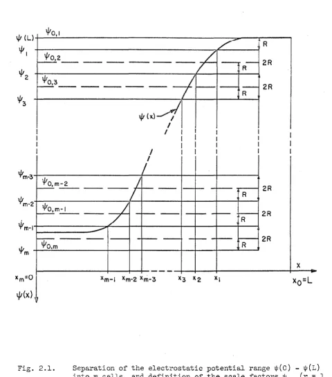
within the allowed range. The situation is illustrated in Fig, 2,1,

The following quantities are then defined

( 2, 11)

r

=

2, 3, • • • m

and are treated as scale factors to allow in each cell r the numerical computation of the integral

L

/J.

J

Hx')-o/or

F (x)

=

e

pr dx'

_'

r

=

1, 2, • • • m

(2.lla)

x

for x

1 ~ x > x . If the following ~uantities are defined as:

r- r

( 2 .12)

r

=

l, 2, • • • m

37

~(L)+--l/J_o,_1 ______________________________ _,,, __ __,~~--,

R

ip I

'4'0,2 _ _ _

1./to,3 __

\f!(x)~

I

I

I I

1./tm~-+---+---+--+--1---1

"10,

m-2

-o/m·2----,,---+---1---1----+---+---1

\ro,m_-_1 _ _ _ .,,._

R

R

2R

2R

2R

2R

2R

x

x₀=L

Fig. 2.1. Separation of the electrostatic potential range ¢(0) - ¢(1) into m cells, and definition of the scale factors ¢

[image:47.613.60.540.150.694.2]

38

[

_{J [}

~(x)-~orj

p ( x)

= (

1-e) F ( _pr x) + Y _pr / z _p e (2.13)

for x

1 ~ x > x

r- r r

=

1, 2, • • • m

where ,,, is selected as the scale factor corresponding to the rth 'Or

cell in which the particular value of x [or ~(x)] is located. It is readily verified that p(x) is scale fa~tor indP.DP.ndP.nt, as desirP.d.

The q_uantities

e

(r

=

2, 3, • • • m) still exceed the permitted range for an applied voltage VA such that

~(O) - t{L) > R

,

*

However, for large enough R , the following inequalities are valid:

y << F (:x:)

pr pr if'

e

<< i if' V(o) - ~(L) > R

Moreover, it can be observed tbat, for a given r, 6 Fpr(x) is either negligible with respect to Ypr' or else comparable to Y ,

pr in which case if ~(O) -

w(L)

> R then x ~ x

1•

The above considerations lead to the following rules:

39

(1) for 0 >VA ~ Vd - R, i.e. low reverse bias, one cell only is present (m

=

1), the parameters ypl and

e

are sufficiently large and equation (2.13) may.be computed in its complete form. (2) for VA < Vd - R the quantity 8 is ignored, and its computation

is not attempted; the parameter y

pr is calculated only in the first cell (r

=

1) since it becomes insignificant elsewhere. With the aid of the above rules, Eq.(2.13) is suitable for an accurate numerical computation of p(x), for an arbitrary reverse bias condition.

A similar procedure leads to an expression extended to high reverse bias cases f'or the electron density. Tht: t:lt:t:L.r·u;:; La.Llc yuLenLla..l range

ijr(O) - ijr(L) is divided into cells defined by:

lst ~t=>ll _Ho) > ~(x) '.> ~

l

(x' ~ 0

0 :5::'. x <"x') .. l

rth cell

w;._i

_{~ w(x) >}

w;

(x' ₁ -::: x < x')

r- r 7

r = 2,

3,

...

m-1 mth cell

V'

_{~ *(x) ~ ~}1 _~

ijr(L) (x' ~ x ~ x' fl L)

m-1 m m-1 m

where

(2 .14)

*I

- ,,,,

= 2R

r-1 'l'r ' r = 2, 3, • • • m

40

~01 ~

*(O)

w;

+

11t;_1

~or

=

2 r = 2, 3, • • • m

the corresponding modified integral

F (x)

~Jx ~

Wor -

1f{x') rlx' nr

0

,

x ' . s x < x ' , · r

r-2 r

(2.15)

1, 2, • • • m

(2 .15a.) may be inserted in Eq.(2.1) to obtain the final expression:

for where:

x' sx <x1

r-l r r = 1, 2, • • • m

/::. [ F

nm (

1)

J

*Or -

~

(

O)

= W' -

* (

L) e ~ Pp

Om

e

z

_n

'it' - HL)

e

om

and 8 is given by relation (2.12).

(2.16)

Considerations similar to those presented in connection with Eq.

(2.13)

lead to the same rules concerning here the parameters

Ynr and

e

in Eq. (2 .16).

41

carrier densities and complete the formulation of the "direct" problem of specifying the applied voltage and solving for the total current a.nd the relevant distributions as functions of position.

The improved formulation for the simplified model is summarized in Table 2 .1.

2.3. Nrunerical techniques.

Once a satisfactory analytical formulation of the problem is achieved, the following phase toward a numerical solution is the dis-cretization of the relevant quantities at a finite number of points. This involves the problem of the distribution of such points throughout the interior of the device, or, in equivalent terms, the determination at each point of the step, defined·as the distance between two

consecu-tive points. In addition, appropriate numerical techniques must be

devised to approximate the analytical integrations and differentiations of the relevant expressions, and to solve the second order linear

differ-ential Eq,(l,45) (essentially Poisson's equation). Theoc topico arc

analyzed in the following subsections.

2.3.1. Automatically adjustable non-uniform step distribution.

It is quite clear f'rom the expected distributions of' most g_uantities

FOHWARD BIAS

L

Ybere: Fin(x) ~

f

e·f(x')dx' x

x

Fn(x) ~

J

.,-t(x' lrlY'

0

Rl!:VERSE BIAS

L

F (x)

e

f

et(x')dx'

Ip x x

Fp(.-) I\

J

.,t(x'l.ix•

0

+' ·t(x)

n(x) ~ ((l-G)F _nr (x) + y _nr ]/(Z _n e or ]

i f , r = l

if' rt l

[

F (0)

J

t(L)·t0r

+clIT-t

~ Pp e

/ e .· cm .

ypr

="'-0

if' r • l

e

· +0r a.nd ·+br• r = l, 2, ••• m a.re sea.le f'actors given by relatione (2,lO), (2.ll), and (2.14), (~.15). R is choaen_as the la.rgeet

mU!lber that i+-UO\ls {L ~ eRt 1 and ( L Pp eRi+ 1 Yitbill the permissible range,

(Z.3)

(Z,4)

(2,lZ)

(z.16)

(2,lJ)

Table 2 ,l, Improved and extended a.rui.lyticfll f'ormuJ.e.tion f'or the aimplif'ied model (obmic contacts,

It is apparent from Fig, 1,4 and Table 2.1 that two main opera-tions are present in the iterative scheme: the integration of the functions e

+

ifr(x) and the solution of Poisson's eQuation. In consid-eration of the accumulative type of error propagation in the execution of a pointwise integration, the former operation is chosen to dictate the criterion responsible for the selection of the step distribution. The integration, in the discretized context, will be performed as a sum of a finite nmr.ber of terms, each computed with the use of an interpolation techni~ue; an error will

oe

introduced in each of such

terms, depending upon the magnitude of' the step a.t Lhe corret>pondent

point for a chosen order of interpolating curve. It is of interest to consider the relative error .ES pertinent to each term, defined as:

relative error of ~ a single term. =

absolute error magnitude of term

A step distribution will be considered optimum if' i t yields the same

relative error for each single term; the.whole integral will then suffer from the same relative error. If this is specified the corres-pondent optimum step distribution can be determined by the procedure illustrated schematically in Fig. 2.2. An upper bound SMx for the step together with the parameter RATIO, the step modifier, may be initially fixed. Starting with the step at its upper bound at the

Assign

e:s

Choose

SVrx: and

RATIO > l

xl = 0 STEPl

=

SMx

i

=

l

Compute the relative error of t~e

integra-+ •1•

tion of e f in the interval x. + S'I'EP.

J_

Decrease the STEP: STEP . ..ci- STEP. /RATIO

J_ J.

Compute the relative error of t~e

integra-+1!1 tion of e · interval

in the x. + STEP.

l. J.

44

C

Proceduxe ) _ E S _ . _ _e,

Increase the STEP: STEP . .._STEP. •RATIO

1 1

45

nu:rrber of points is obtained.

The two integrands e+

~(x)

will in general generate two different step distributions; it is appropriate to choose at each point the most severe step requirement featured by the two distributions.

It is very convenient to proceed one stage further by linkine, in reverse order, the relative error with the desired total number of points .j',. This latter parameter is directly related to the storage

capability of the particular machine available (and to the actual computation time), therefore it may be inserted externally as input

DATA to suit the particular needs of' the prog.eamnieL', When .(, 11::>

specified, the problem consists in determining ES' which allows then the generation of the step distribution with the aid of the procedure

discussed above. This can be achieved with nn interpolation scheme of

the type illustrated in Fig. 2.3. A few trials with suitable values of ES will determine the correspondent t values to surround the required number of points ~ by two t values; at this point successive

Lagrangian interpolations may be used on- the curve e:S =

Es (

t) to complete the search of the relative error (e:₈)R correspondent to tR.

Two different approaches may be taken for the actual pointwise computation of the relative error to be compared with the specified e:

3,

depending upon the availability of the function ~(x) in discretized or analytical form.

Assic;n ~

Choose lnlLlal £

8 j

=

1

BRANCH

=

0 Procedure

~ ~ -?

<-s J

YES---:::~::~-::;-;;---­

_BRANCH

₌

_l?

YES

Is

t

(j-l) < ~ < t(j)

or

t(j-l) > tR > t(j)? YES BRANCH

=

1

Use Lagrangian interpolation on the curve

Es

= Es(t),

in search for the (£₈)R corres-ponding to tR. Obtain a new

Decrease £8

YES

Increase

ES

Fig, 2.3, Pru<..:t:clurt: t1u.lLable to obtain the step distribution and the relative error £

47

'¥(j)(x). If the correction &(j+l)(x) is significant, a new step

U.ie>tribution may be desirable. In this cast:: th1:: following o.l.gorll.,hm

may be used to. obtain the relative error at each point.

Let Si be the step at the point of abscissa xi' defined as

i = 1, 2, 3, ••• .t-1

where xi = O, x~ = L. In the execution of one sweep from 0 to L

the steps

s

_r r

=

1,.. 2,.. • • • i-1

are supposed already adjusted to the proper value; the adjustment of the step S. is sought. Moreover, for ·simplicity, let the trapezoidal

J..

rule be chosen for the numerical integration of the function f(x);

an elementary contribution amounts, in the present case, to the area between points x., x. 1 under the curve 1 1+ ' f(x) (see Fig, 2.4). This

value must be compared with the exact one, which, for all practical purposes, may be computed with the use of a higher order interpolating curve, for example by tracing a cubic through the points _{f. J.'}

1

-f. ₁₊ l' f. _l.+ 2' and by integrating it between x₁ and x. _{l.+ 1} (see

Appendix B for explicit relations). Result of the comparison may cause a shift in x.

1 to a new ~osition

l.+ ~. x' _i+J.' . the correspondent value

Fig. 2.4.

48

third order polynomial

Xj-1 X· I

_{I .}

I

Xj +1

I

Xj +1

x

Shift of the point x.

1 to achieve the required integration error and det.ermine Hie step size at the point x .•