Computational Solutions of Two Dimensional Convection Diffusion Equation Using Crank Nicolson and Time Efficient ADI

(1)

http://www.scirp.org/journal/ajcm ISSN Online: 2161-1211

ISSN Print: 2161-1203

DOI: 10.4236/ajcm.2017.73019 Aug. 3, 2017 208 American Journal of Computational Mathematics

Computational Solutions of Two Dimensional

Convection Diffusion Equation Using

Crank-Nicolson and Time Efficient ADI

Muhammad Saqib, Shahid Hasnain, Daoud Suleiman Mashat

Department of Mathematics, Numerical Analysis, King Abdulaziz University, Jeddah, Saudi Arabia

Abstract

To develop an efficient numerical scheme for two-dimensional convection diffusion equation using Crank-Nicholson and ADI, time-dependent nonli-near system is discussed. These schemes are of second order accurate in apace and time solved at each time level. The procedure was combined with Iterative methods to solve non-linear systems. Efficiency and accuracy are studied in term of L2, L∞ norms confirmed by numerical results by choosing two test examples. Numerical results show that proposed alternating direction implicit scheme was very efficient and reliable for solving two dimensional nonlinear convection diffusion equation. The proposed methods can be implemented for solving non-linear problems arising in engineering and physics.

Keywords

Crank-Nicholson, Taylor’s Series, Newton’s Iterative Method, Alternating Direction Implicit (ADI)

1. Introduction

In this paper we have extended our previous approach associated to two dimension Convection-diffusion equation. The great Physicist Johannes Martinus Burgers discovered Burgers equation, which is non-linear parabolic partial differential equation (PDE) and widely used as a model in many engineering problems, which explains such as physical flow phenomena in fluid dynamics, turbulence, boundary layer behavior, shock wave formation, and mass transport [1]. Two dimensional convection-diffusion equation is given by the following equation.

(

)

1

0

t x y xx yy

u uu uu u u

R

+ + − + =

(1)

How to cite this paper: Saqib, M., Has-nain, S. and Mashat, D.S. (2017) Computa-tional Solutions of Two Dimensional Con-vection Diffusion Equation Using Crank- Nicolson and Time Efficient ADI. Ameri-can Journal of Computational Mathemat-ics, 7, 208-227.

https://doi.org/10.4236/ajcm.2017.73019

Received: February 23, 2017 Accepted: July 31, 2017 Published: August 3, 2017

(2)

DOI: 10.4236/ajcm.2017.73019 209 American Journal of Computational Mathematics

where

(

x y t

, ,

)

∈Ω×

(

0,

T

]

with initial conditions

(

, , 0

)

0

( ) ( )

,

u x y

=

u x y

x y

∈Ω

The Dirichlet boundary conditions are given by

(

, ,

)

1

(

, , ,

)

(

, ,

)

2

(

, ,

)

u a y t

=

f x y t

u b y t

=

f

x y t

(

, ,

)

1

(

, , ,

)

(

, ,

)

2

(

, ,

)

u x c t

=

g x y t

u x d t

=

g

x y t

where

(

x y t

, ,

)

∈Ω×

(

0,

T

]

, Ω =

{

(

x y,

)

:a≤ ≤x b c, ≤ ≤y d

}

is a rectangular domain in 2

R

,

(

0,

T

]

is the time interval. u₀,f f g g₁, ₂, ₁, ₂ are given sufficiently

smooth functions and

u x y t

(

, ,

)

may represent heat, diffusion, etc. Re is the

Reynolds number.

This equation established the interaction between the non-linear convection processes and the diffusive viscous processes [2]. As Burgers equation is probably one of the simplest non-linear PDE for which it is possible to obtain an exact solution [3]. Also depending on the magnitude of the various terms in Burgers equation, it behaves as an elliptic, parabolic or hyperbolic PDE, conse- quently, it is one of the principle model equations used to test the accuracy of new numerical methods or computational algorithms [4]. It is widely known that non-linear PDEs do not have precise analytic solutions [5]. The first attempt to solve the Burgers equation analytically was done by Batman [6], who derived the steady state solution of this equation as a test solution to one dimension, which was used to model turbulence nature of the phenomena [7][8]. The two dimensional non-linear Burgers equations are a special form of in compressible Naiver-Stokes equations without the pressure term and the continuity equation

[9][10]. Due to its wide range of applicability, several researchers, both scientists and engineers, have been interested in studying the properties of the Burgers equation using various numerical techniques [11]. They have successfully used it to develop new computational algorithms and to test the existing ones [12]. Vineet and Tamsir [10] used two different test problems to analyses the accuracy of the Crank Nicholson(CN) scheme [10]. From literature review, it came to know that Newton’s method is also applicable to reform the Jacobean matrix to get the linear algebraic sparse matrix. Solution of such algebraic system of equations can be found by Gauss elimination with partial pivoting technique [13] [14]. Bahadir also used same technique to test the accuracy of scheme, using fully implicit finite difference scheme [15][16]. The terminology of the Burgers equation explains that with viscous term the Burgers Equation is parabolic while without viscous term it is hyperbolic. In the later case it possesses discontinuous solutions due to the non-linear term and even if smooth initial condition is considered the solution may be discontinuous after finite time [8]. It also governs the phenomenon of shock waves [12].

(3)

equations into parabolic partial differential equation [17]. Some of the researchers also tried to tackle the non-linear Burgers equation directly (without Hopf-Cole transformation), by applying Crank-Nicholson finite difference method to the linearized Burgers equation by Hopf-Cole transformation which is unconditionally stable and is second order convergent, in both space and time with no restriction on mesh size [10]. In another result due to Kutluay et al. a direct approach via least square quadratic B-spline finite element method is discussed [18]. Recently Pandey et al. discussed Douglas finite difference scheme on linearized Burgers equation which is fourth order convergent in space and second order convergent in time [1][18].

1.1. Problem 1

From literature review, [19] we found that earlier work done by Mittal,Jain and Holla in 2012 [20] on convection-diffusion equation in one dimension. We extended our work to enhance our knowledge towards two dimensional Convection diffusion equation.Two test problems were taken to understand the numerical solution with finite difference schemes. By setting some parameters with arbitrary constants in bounded domain Ω =

{

(

x y,

)

: 0.5− ≤ ≤x 0.5, 0.5− ≤ ≤y 0.5

}

. Exact

solution of the above two dimensional equation is

(

, ,

)

0.5 tanh

(

)

2

x y t R

u x y t = − _ + − _

 (2)

where

( )

x y

,

∈Ω

, t>0 and R is a parameter, known as Reynolds number.

Boundary conditions and initial conditions can be taken from exact solution of u(x,y,t) [21].

1.2. Problem 2

In this problem the rectangular domain of two dimensional nonlinear convection- diffusion Equation (1) is given as Ω =_

(

x y,

)

: 0≤ ≤x 1, 0≤ ≤y 1_ . Exact

solution of the above two dimensional equation is

(

)

₍

1

₎

, , 1

2

u x y t

x y t R

=

+ − +

(3)

where

( )

x y

,

∈Ω

, t>0 and R is a parameter, known as Reynolds number.

Boundary conditions and initial conditions can be taken from exact solution of

(

, ,

)

u x y t

. where Ω is a rectangular domain in

_R

2_{. The main objective of the} paper is to find efficient solution of unknown

u x t

( )

,

. Two test problems were

described to understand the numerical solution by taking two finite difference schemes. Also Convection diffusion equation has been extensively studied to describe various kinds of phenomena which can be seen from equation [21].

2. Numerical Methods

(4)

domain Ω. The first step is to choose integers L and M to define step sizes

(

)

hx

= −

b a L

and

hy

=

(

d

−

c M

)

in x and y directions respectively.

Partition the interval [a, b] into L equal parts of width hx and the interval [c, d]

into M equal parts of width hy. Place a grid by drawing vertical and horizontal

lines through the points with coordinates

(

x y

l

,

m

)

, where xl = +a lh for each

0,1, 2,

,

l

=



L

and y_m = +c mk for each m=0,1, 2,,M also the lines

l

x=x and y=ym are grid lines, and their intersections are the mesh points of

the grid. For each mesh point in the interior of the grid,

(

x y

_l

,

_m

)

, for

1, 2,

,

1 l

=



L

−

and m=1, 2,,M −1 , we apply different algorithms to

approximate the numerical solution to the problem in equation [21] also we assume tn =nk n, =0,1,,NT where t is the time.

2.1. Second Order Implicit Scheme

We apply Crank-Nicholson implicit finite difference scheme to equation [21], by integrating Equation (1) in the compact way:

1 1

, , , ,

1 1 1 1

1, 1, 1, 1, , 1 , 1 , 1 , 1

1, , 1, , 1 , , 1

2 2 2 2 , 2 , 4 4

ˆ 2ˆ ˆ ˆ 2ˆ ˆ

ˆ , ˆ

n n n n

l m l m l m l m

t

n n n n n n n n

l m l m l m l m l m l m l m l m

x y

l m l m l m l m l m l m

x y

u u u u

u u

k

u u u u u u u u

u u

h h

u u u u u u

u u h h

δ

+ + + + + + + − + − + − + − + − + −  + + = =    − + − − + − _ = =   − + − +  = = _ 

when substitute these terms in to Equation (1), the Crank-Nicholson Scheme is given by

(

){

}

1 1 1 1 1 1

, , 1 , , 1, 1, 1, 1, , 1 , 1 , 1 , 1

1 1 1 1 1

2 1, 1, , 1 , 1 4 , 1, 1, , 1 , 1 4 , 0

n n n n n n n n n n n n

l m l m l m l m l m l m l m l m l m l m l m l m

n n n n n n n n n n

l m l m l m l m l m l m l m l m l m l m

u u R u u u u u u u u u u

R u u u u u u u u u u

+ + + + + + + − + − + − + − + + + + + + − + − + − + −   − + _ + − + − + − + − _   + _ + + + − + + + + − _=

1 2 2

where , 8 2 k k R R h Rh = = (4)

The scheme shows that the accuracy is of

(

2 2

)

O k +h . A Jacobian matrix is now Penta-diagonal, but unfortunately due to large number of iterations it extends from the diagonal at least n entries away in every direction,but another methods which can be used to handle such problems (discussed later), because of the large bandwidth, increasing grid points the calculation become more difficult. To overcome this difficulty another method solution is needed.Newton method is used for solving nonlinear task (discussed later). The Crank- Nicholson is computationally inefficient.

2.2. Computationally Efficient Implicit Scheme

(5)

In this approach, the finite difference equations are written in terms of quantities at two levels However, two different finite difference approximations were used alternately, one to advance the calculations from the plane n to a plane n*, and the second to advance the calculations from (n*)-plane to the (n + 1). Same parameters were used in this method as described above. The derivation of ADI scheme, we have following steps;

Sweep in x-direction

(

)

(

)

(

)

(

)

(

)

* * * *

, , 1 1, , 1, 1, , 1,

2 , 1 , 1, 3 , 1, 1,

3 , , 1 , 1

2 2

2

n n n n

l m l m l m l m l m l m l m l m

n n n n n n

l m l m l m l m l m l m

n n n

l m l m l m

u u P u u u u u u

P u u u P u u u

P u u u

+ − + − + − + − + − − = − + + − + + − + + − + − (5)

(

)

(

)

(

( )

)

( )

* 2 * 2

, , 1 , , 2 ,

n n n n

l m l m x l m l m y l m

u −u =P δ u +u +P δ u +kF u

(6) where

( )

3

(

,

( )

,

)

3

(

, ,

)

n n n n n

l m x l m l m y l m F u =P u δ u +P u δ u

Sweep in y-direction

(

)

(

)

(

)

(

)

(

)

1 * 1 1 1 * * *

, , 1 , 1 , , 1 , 1 , , 1

* * * * * *

2 1, , 1, 3 , 1, 1,

* * *

3 , , 1 , 1

2 2

2

n n n n

l m l m l m l m l m l m l m l m

l m l m l m l m l m l m

l m l m l m

u u P u u u u u u

P u u u P u u u

P u u u

+ + + + + − + − + − + − + − − = − + + − + + − + + −

+ − (7)

(

)

(

)

(

( )

)

( )

1 * 2 1 * 2 * *

, , 1 , , 2 ,

n n

l m l m y l m l m x l m

u + −u =P δ u + +u +P δ u +kF u (8)

where

( )

*

(

*

( )

*

)

(

* *

)

3 l m, x l m, 3 l m, y l m, F u =P u δ u +P u δ u

1 2, 2 2, 3

2 2

k k k

P P P

h

Re h Reh

= = =

where * ,

l m

u defines similarly to 1 ,

n l m

u + . This method is unconditionally stable.

The method has accuracy

(

2 2

)

O k +h , newton’s iterative method is used to solve tridiagonal system.

The family of linear system in x-direction as:

(

)

*

1 , 1 ,

u n

x m m x m

a u =b +F ku

(9) where m=1,,M−1

The family of linear system in y-direction as:

(

)

1 *

1 , 1 ,

n

y m m y m

c u + =d +F ku

(10) where

l

=

1,



,

L

−

1

where a c1, 1 develops tridiagonal matrix and the array b d1, 1 depends on l and m

The reaction term is x-direction

(

,

)

( )

1, , ,

(

1, 1

)

n n n

x m m L

F ku = kF u  kF u − _

(6)

( )

*

(

*

)

( )

*

, 1, 1 , , 1,1

y l M

F ku = kF u −  kF u 

finally the scheme makes tridiagonal family of linear system.Iterative methods was carried out to solved this system. The trick used in constructing the ADI scheme is to split time step into two, and apply two different stencils in each half time step, therefore to increment time by one time step in grid point, we first compute both of these stencils are chosen such that the resulting linear system is tridiagonal [5][7][8] [9][11] [17][22]. To obtain the numerical solution, we need to solve a non-linear tridiagonal system at each time step. We have done this by using Newton’s iterative method

Algorithm 1

To construct Newton iterative method for the two dimensional Convection- diffusion equation. The non-linear system in equations [23] and [24], can be written in the form:

( )

0 G S

=

₍₁₁₎

where

( )

T 1

1, , 2, , , 2 2 ,

n

m m L m

S≈_u + _{ }=S S  S ₋ _ T

1 1 1 1 1

1, 2, 3, 1,

: , , , ,

n n n n n

m m m L m

m

u + = u+ u+ u+ u +− 

( )

T 1,m, 2,m, , 2L 2 ,m

G= G G  G ₋ _ , where G_1,_m,G_2,_m,,G₍₂_L₋_{2 ,}₎_m were system of

nonlinear equations obtained from the system in [23] and [24]. The system of equations, is solved by Newton’s iterative method using the following steps

1) Specify ( )0

u as an initial approximation.

2) For

k

=

0,1, 2,



until convergence achieve.

• _{Solve the linear system}

( )

( )k ( )k

( )

( )k A u ∆u = −R u

• _Specify (k 1) ( )k ( )k u + =u + ∆u ,

where

( )

( )k

A u is

(

m m

×

)

Jacobian matrix, which is computed analytically and ( )k

u

∆ _{is the correction vector. In the iteration method solution at the previous}

time step is taken as the initial guess. Iteration at each time step is stopped when

( )

k

R u Tol

∞ ≤ with Tol is a very small prescribed value. The linear system

obtained from Newton’s iterative method, is solved by Court’s method. Convergence done with iterations along less CPU time [5][14].

Algorithm 2

Clearly, the system is tridiagonal and can be solved with Thomas algorithm. The dimension of J is l×m. In general a tridiagonal system can be written as,

1 1 , with 1 0

l l l l l l l l

a x− +b x +c x+ =S a = =c

above system can be written as in a matrix-vector form, Ju=S

(7)

1 1

2 2 2

1 1 1

0 0 0 0

0 0 0

n n n

n n

b c

a b c

J

a b c

a b − − −           =                                       

[

1, 2, 3, ,

]

t n

u= u u u  u

[

1, 2, 3, ,

]

t n

S= s s s  s

technique is explained in the following steps, J=LU

where

1

2 2

3 3 3

1 1 1

0 0 0 0 0

0 0 0 0

0 0 0

0 0

n n n

L µ β µ

α β µ

− − −         =                           and 1 1 2 2 3 3 2 2 1

1 0 0 0

0 1 0 0

0 0 1 0

0

... 0 1

0 0 1

n n U δ λ δ λ δ λ δ λ δ − −           =                           

By equating both sides of the Ju=S, we get the elements of the matrices L

and U. The computational tricks for the implementation of Thomas algorithm are shown in results, taken from a specific examples.

3. Error Norms

The accuracy and consistency of the schemes is measured in terms of error norms specially L2 and L∞ which are defined as:

(

)

2

, , , 1

L

i j i j i j U u RMSError L L = − = ×

∑

(12)

(

. ,

)

1 1 max L

i j i j i L

j

L∞ _{≤ ≤} U u

=

∑

− ₍₁₃₎

(

) (

)

2 , , , ,

t

i j i j i j i j L =

ρ

U −u U −u

(8)

where

u x y t

(

, ,

)

and

U x y t

(

, ,

)

denote the numerical and exact solutions at

the grid point

(

x y t

_l

,

_m

,

_n

)

. In this method ρ

(

U_{i j}_, −u_{i j}_,

)

=max

( )

λ and λ is

an eigen value of

(

Ui j, −ui j,

)

respectively.

4. Results and Discussion

Numerical computations were performed using the uniform grid. In Table 1 &

Table 2 Crank-Nicholson and ADI results was performed, compared with the analytical results at grids size 20

×

20 in problem 1. Moreover by fixing some parameter such as time step k = 0.0001 time level t = 0.5 and Reynolds number

Re = 100,500 with different mesh points. The obtained results was compared with the existing results in literature. By describing results same parameters, notations was used as other researchers were used in their studies. For convergence L L2, ∞ norm were used for the unknown

u x y t

(

, ,

)

Khater et al. (2008), Mittal and Jiwari (2012), Kutluay and Yagmurlu (2012) and R.C. Mittal and Amit Tripathi were considered this problem in (2016) [21] [23] [24]. Approximate results in problem 1 Table 3, comparison of analytical and numerical results of CN and ADI at fixed Reynolds no Re = 500, time level = 0.0005, time = 1, grid size 30 × 30 with different typical mesh points at (-0.3,-0.3), (−0.45, −0.45), (−0.35, −0.35), (0.25, −0.25). The obtained results makes a very good agreement with the exact solution. To attain more refine and better results by changing time level = 0.001, grid size = 25 × 25 with the same mesh points in

Table 4 more refine results was obtained with Reynolds no Re = 50. In Figure 1

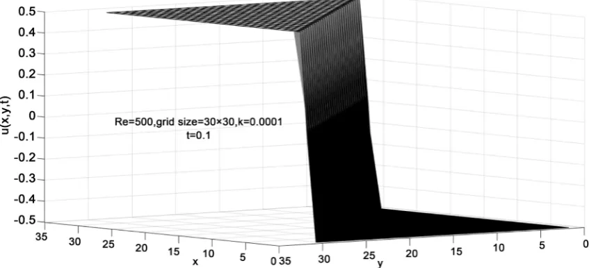
analytical and numerical results were compared at grid size 20 × 20 k = 0.0001 time = 0.5 and time level = 0.0001 corresponding results in Table 1. Figure 2

and Figure 3 changing time = 0.1 and grid size 30 × 30 with same time level and Reynolds no as in Figure 1. In both Figure 1 and Figure 2 almost same behavior corresponds to results in Tables 1-4. Similar patterns were depicted by Kutluay and Yagmurlu (2012), Mittal (2016) [21] [24]. The obtained solutions were better than those obtained in earlier studies (Khater et al., 2008; Kutluay and Yagmurlu, 2012, Mittal (2016).

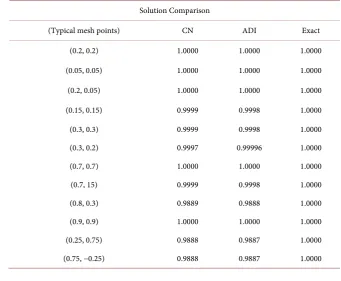
In problem 2, considering Equation (1) over the domain [0.5, 0.5] × [0.5, 0.5], boundary and initial conditions were taken from the exact solution showed stable results time step and increasing grid size (refine mesh size). In Table 5

analytical and numerical results of Crank-Nicholson and ADI were compared at gird size 30 × 30, Re = 200, time = 1, time step = 0.001. In problem 2, Table 6 by reducing grid size 20 × 20, increasing time step k = 0.0001 and time = 3 with fixed Reynolds number attained stable results.

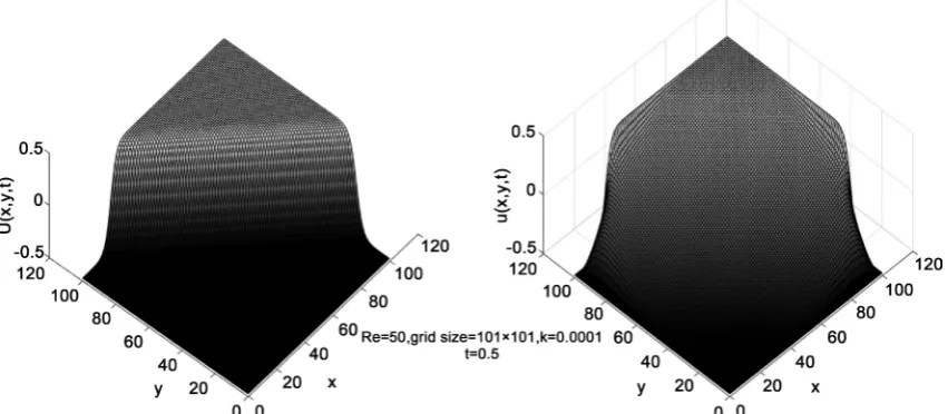
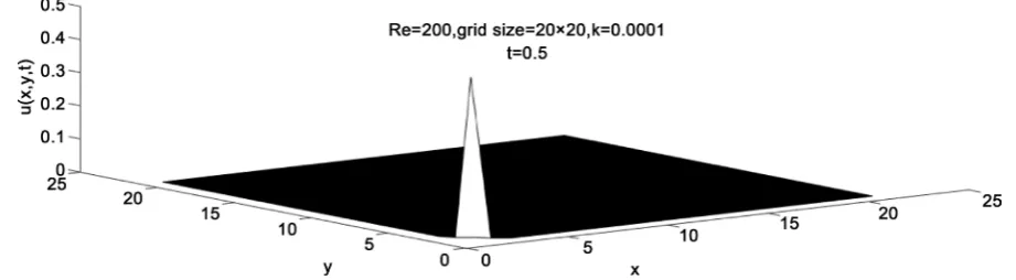
In Figure 4 showed ADI results by reducing Reynolds no Re = 10 with gird size 20 × 20 k = 0.0001 and time = 0.5 and in Figure 5 increasing grid size 101 × 101 at Reynolds 50, time level = 0.0001, time = 0.5, obtained good accuracy corresponds to the exact results.Matrices 2

x

δ _and 2

y

(9)

[image:9.595.207.539.118.396.2]

Table 1. Comparison of Analytical and Exact solution at different time level with fixed Reynolds number Re = 100 at t = 0.5, k = 0.0001 and grid size = 20 × 20 for unknown

(

, ,

)

u x y t Problem 1.

Solution Comparison

(Typical mesh points) CN ADI Exact (−0.3, −0.3) −0.5000 −0.5000 −0.5000 (−0.45, −0.45) −0.49999 −0.5000 −0.5000 (−0.3, −0.45) −0.49999 −0.49999 −0.5000 (−0.35, −0.35) −0.49998 −0.49997 −0.5000 (−0.25, 0.25) 0.0000 −0.0000 0.0000

(−0.2, −0.2) −0.49997 −0.49888 −0.5000 (−0.2, −0.3) 0.49997 0.49888 0.5000

(0.2, 0.2) 0.49998 0.49998 0.5000 (0.2, 0.35) −0.49999 −0.49999 −0.5000

(0.3, 0.2) 0.49999 0.49777 0.5000 (0.25, −0.25) 0.0000 0.0000 0.0000 (0.4, 0.4) 0.5000 0.5000 0.5000

Table 2. Comparison of Analytical and Exact solution at different time level with fixed Reynolds number Re = 500 at t = 0.5, k = 0.0001 and grid size = 20 × 20 for unknown

(

, ,

)

Solution Comparison

(Typical mesh points) CN ADI Exact (−0.3, −0.3) −0.50000 −0.50000 −0.5000 (−0.45, −0.45) −0.48999 −0.50000 −0.5000 (−0.3, −0.45) −0.48999 −0.489999 −0.5000 (−0.35, −0.35) −0.48998 −0.489997 −0.5000 (−0.25, 0.25) 0.00000 −0.00000 0.0000

(−0.2, −0.2) −0.489997 −0.489888 −0.5000 (−0.2, −0.3) 0.489997 0.489888 0.5000

(0.2, 0.2) 0.489998 0.489998 0.5000 (0.2, 0.35) −0.489999 −0.489999 −0.5000

[image:9.595.201.541.456.735.2]

(10)

[image:10.595.208.539.117.397.2]

Table 3. Comparison of Analytical and Exact solution at different time level with fixed Reynolds number Re = 500 at t = 1, k = 0.0005 and grid size = 30 × 30 for unknown

(

, ,

)

u x y t .

Solution Comparison

(Typical mesh points) CN ADI Exact (−0.3, −0.3) −0.50000 −0.50000 −0.5000 (−0.45, −0.45) −0.49999 −0.50000 −0.5000 (−0.3, −0.45) −0.49999 −0.489999 −0.5000 (−0.35, −0.35) −0.49998 −0.489997 −0.5000 (−0.25, 0.25) −0.49997 −0.49997 −0.5000 (−0.2, −0.2) −0.499997 −0.489888 −0.5000 (−0.2, −0.3) −0.499997 −0.489888 −0.5000 (0.2, 0.2) −0.499998 −0.489998 −0.5000 (0.2, 0.35) −0.499999 −0.489999 −0.5000 (0.3, 0.2) −0.499999 −0.489777 −0.5000 (0.25, −0.25) −0.49999 −0.49999 −0.5000 (0.4, 0.4) −0.50000 −0.50000 −0.5000

(

, ,

)

Solution Comparison

[image:10.595.208.540.457.725.2]

(11)

[image:11.595.110.541.69.258.2]

[image:11.595.120.543.292.474.2]

Figure 1. Analytical and numerical results of CN at t = 0.5, grid size = 20 × 20, k = 0.0001, Re = 500 problem 1.

Figure 2. Numerial results of CN at t = 0.1, grid size = 30 × 30, k = 0.0001, Re = 500 problem 1.

[image:11.595.114.543.511.704.2]

(12)

[image:12.595.208.539.118.397.2]

(

, ,

)

Solution Comparison

(Typical mesh points) CN ADI Exact (0.2, 0.2) 1.0000 1.0000 1.0000 (0.05, 0.05) 0.9996 0.9887 1.0000 (0.2, 0.05) 0.9765 0.9665 1.0000 (0.15, 0.15) 0.8514 0.8661 1.0000 (0.3, 0.3) 0.8515 0.8415 1.0000 (0.3, 0.2) 0.9000 0.9112 1.0000 (0.7, 0.7) 0.7515 0.7414 1.0000 (0.7, 15) 0.8775 0.8675 0.9987 (0.8, 0.3) 0.9876 0.9866 1.0000 (0.9, 0.9) 0.9996 0.9954 1.0000 (0.25, 0.75) 0.0000 0.0000 0.0000 (0.75, −0.25) 1.0000 1.0000 1.0000

(

, ,

)

Solution Comparison

[image:12.595.198.540.455.736.2]

(13)

[image:13.595.96.500.66.208.2]

[image:13.595.87.513.241.427.2]

Figure 4. Numerical results of ADI at t = 0.5, grid size = 20 × 20, k = 0.0001, Re = 10 problem 1.

Figure 5. Analytical and numerical results of ADI at t = 0.5, grid size = 101 × 101, k = 0.0001, Re = 50 problem 1.

Table 7. Calculating errors using different parameters for unknown values u(x, t) at different grid size and time step k at t = 0.05, Re = 1 Problem 2.

k grid size L2 L∞ Mittal [21] L2 Mittal [21] L∞ Khater [23] L2 Khater [23] L∞ 0.005 5 5× 4.9586e−007 5.9234e−007 4.9688e−008 4.6512e−008 1.19e−007 8.94e−008 0.0005 10 10× 6.1723e−007 6.6123e−007 6.2171e−009 5.9068e−009 8.05e−007 7.45e−007 0.0001 15 15× 2.1132e−008 3.1324e−008 2.5318e−009 2.188e−009 .... .... 0.0001 30 30× 1.2654e−008 2.2131e−008 1.8750e−009 1.0101e−009 ... ...

Table 8. Calculating errors using different parameters for unknown values u(x, t) at different grid size and time step k at t = 0.25, Re = 1 Problem 2.

[image:13.595.57.541.489.588.2] [image:13.595.55.539.632.732.2]

(14)

Table 9. Calculating Errors using different parameters for unknown values u x t

( )

, at

different grid size at k = 0.005, t = 0, Re = 100 Problem 1.

grid size L2 L∞ Mittal [21] L2 Mittal [21] L∞ Rms 5 5× 4.5112e−016 3.4661e−016 5.4017e−017 4.5997e−017 4.5112e−016 11 11× 2.3451e−016 1.5712e−016 3.6338−017 2.6712e−017 2.3451e−016 21 21× 1.0231e−017 1.0321e−017 1.2898e−017 1.1275e−017 1.0231e−017

Table 10. Calculating Errors using different parameters for unknown values u x t

( )

, at

different grid size at k = 0.005, t = 0.05, Re = 100 Problem 1.

grid size L2 L∞ Mittal [21] L2 Mittal [21] L∞ Rms

5 5× 4.41172e−005 3.8761e−005 5.0688e−006 4.9850e−006 4.41172e−005 11 11× 2.3151e−005 2.9712e−005 3.4403e−006 3.2143e−006 2.3151e−005 21 21× 1.0931e−006 1.0991e−006 2.3549e−006 2.0547e−006 1.0931e−006

size and grid size with fixed Reynolds no Re = 1, t = 0.05 and 0.25. Good results obtained when compared the values of this exact solution with those of the approximation gained in Tables 1-3. Furthermore in Table 9 error reduced when changing grid size at fixed Reynolds no Re = 100,k = 0.005, time = 0 .In our next computations in Table 10 changing Reynolds no Re and grid size at time = 0.1 error increased. It means that error increase by choosing high Reynolds no Re value.Solution profiles at t = 0.5 and t = 1 have been presented in Figure 6 and Figure 7 for grids sizes 20 × 20 and 30 × 30 at k = 0.001, Re = 50 and 100 respectively. Figure 8 Crank-Nicholson results obtained using same parameters as in Figure 7 with grid size 25 × 25. Solution presented in Figure 9

at grid point 20 × 20, time = 0.5, step size = 0.0001 with large Reynolds no Re = 200 error increased. Solution reported in Table 11 by changing Reynolds no Re and grid sizes at time = 0.1 and k = 0.001, 0.0001 L L2, ∞ norm increased. Root mean square value also increased by changing Reynolds no Re. Among all the interior grid points found both L L2, ∞ norm of the numerical solution. Figure 10 was presented at grid time = 1, k = 0.001, showed maximum results at time = 0.5. Approximate solution compare with exact of ADI presented in Figure 11

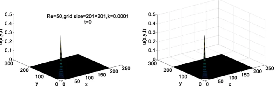
and Figure 12 with grid size 30 × 30 and 20 × 20, time = 2 and 1 respectively. In these figure choosing low Reynolds no Re = 10 at k = 0.0001 presents very refine results in time efficient manner. In Figure 13 by refining mesh sizes showing excellent results at k = 0.0001, Re = 10 and grid sizes 101 × 101. Solution presents in Figure 14 at time = 0 makes a good agreement with the exact solution at time step = 0.0001, Re = 50 respectively.

(15)

[image:15.595.63.544.71.248.2]

[image:15.595.58.551.286.440.2]

Figure 6. Numerical results of ADI at t = 0.5, grid size = 20 × 20, k = 0.001, Re = 100 problem 1.

Figure 7. Numerical results of ADI at t = 1, grid size = 30 × 30, k = 0.001, Re = 50 problem 1.

[image:15.595.64.534.474.705.2]

(16)

[image:16.595.67.528.72.199.2]

[image:16.595.55.529.260.503.2]

Figure 9. Numerical results of CN at t = 0.5, grid size = 20 × 20, k = 0.0001, Re = 200 problem 2.

Table 11. Calculating errors using different parameters for unknown values u x t

( )

, at different Reynold’s number, grid sizes at t

= 0.1 Problem 1.

Re grid size k L2 L∞ Mittal [21] L2 Mittal [21] L∞ Rms

100 21 21× 0.001 6.1601e−005 5.9645e−005 7.1536e−006 6.9729e−006 6.1601e−005

[image:16.595.99.498.534.700.2]

300 101 101× 0.0001 7.2134e−004 7.1206e−004 8.2579e−005 8.1304e−005 7.2134e−004 500 201 201× 0.0001 2.6145e−004 1.4172e−004 3.6692e−004 2.4573e−004 2.6145e−004

Figure 10. Numerical results of CN at t = 1, grid size = 30 × 30, k = 0.001, Re = 50 problem 2.

(17)

[image:17.595.81.525.76.278.2]

[image:17.595.70.528.317.523.2]

Figure 12. Exact and numerical results of ADI at t = 1, grid size = 30 × 30, k = 0.0001, Re = 10 problem 2.

Figure 13. Analytical and numerical results of ADI at t = 2, grid size = 20 × 20, k = 0.0001, Re = 10 problem 2.

[image:17.595.70.535.557.706.2]

(18)

have been obtained in earlier studies (Mittal and Jiwari, 2016). In literature point of view present schemes shows similar results as (Jain and Holla, 1978; Mittal and Jiwari, 2016, khater (2008)) [21] [23]. Moreover, got similar results with small grid size. From graphical illustrations, obtained numerical results give steady state solution and the scheme is stable. In Table 9 & Table 10 we observed that results becomes better by changing grid sizes from low to high and by reducing step size.

The obtained results gives excellent agreement with the solutions available in the literature. When the number of grid points get larger than several hundred, the memory and storage of the Crank-Nicholson starts to become a serious issue and it is better to solve this method using different approaches that take advantage of the special form. This method is computationally inefficient. Thomas algorithm avoids having to store having the whole matrix J (Jacobean) in its memory and solve the system much more expediently. ADI methods reduces to the CN scheme and this method solve the system very efficiently.The order of truncation error: _O

(

_k2₊_h2

)

. The implementation of ADI computa-

tionally is in a time efficient manner. Alternating direction implicit method is fastest when it works and it works well for simple,ideal problems and give efficient results.

5. Conclusion

In this research work, finite difference methods has been discussed for solving two dimensional convection-diffusion equation. Two test problems were considered, explained the efficiency, accuracy and stability of the schemes. The numerical results showed that Alternating Direction Implicit method is easy to implement and excellent in time efficient manner. The accuracy and stability of these methods were compared to the other numerical methods, shows good agreement with the exact solution. Both ADI and Crank-Nicholson are unconditionally stable and highly accurate. For convergence L2 and L∞ norms

were treated towards zero when grid size was increased. Numerical results showed that both methods are good but ADI method is consistent and time- efficient. The approach used in this paper may be useful to solve higher dimensional partial differential equations appearing in various applications of science and engineering.

Acknowledgements

(19)

Competing Interests

This paper has no financial or non-financial competing interest.

Authors Contribution

The authors contributed to the manuscripts equally.

References

[1] Pandey, K.P., Lajja, V.L. and Amit, K.V. (2009) On a Finite Difference Scheme for Burgers Equation. Applied Mathematics and Computation, 215, 2208-2214.

https://doi.org/10.1016/j.amc.2009.08.018

[2] Fletcher, C.A. (1983) Generating Exact Solutions of the Two-Dimensional Burgers Equations. International Journal for Numerical Methods in Fluids, 3, 213-216.

https://doi.org/10.1002/fld.1650030302

[3] Collatz, L.C. (1960) The Numerical Treatment of Differential Equations. Springer Verlag, Berlin, 28. https://doi.org/10.1007/978-3-662-05500-7

[4] Zhu, H.Q., Shu, H.Z. and Ding, M.Y. (2010) Numerical Solution of Two-Dimen- sional Burgers’ Equations by Discrete Adomian Decomposition Method. Comput-ers and Mathematics with Applications, 60, 840-848.

https://doi.org/10.1016/j.camwa.2010.05.031

[5] Mazumder, S.M. (2015) Numerical Methods for Partial Differential Equations: Fi-nite Difference and FiFi-nite Volume Methods. Academic Press, New York.

[6] Bateman, H.B. (1915) Some Recent Researches on the Motion of Fluids. Monthly Weather Review, 43, 163-170.

https://doi.org/10.1175/1520-0493(1915)43<163:SRROTM>2.0.CO;2

[7] Crandall, S.H. (1956) Engineering Analysis. McGraw-Hill,New York, 151. [8] Noye, J.N. (1981) Nonlinear Partial Differential Equations in Engineering.

Univer-sity of Melbourne, Melbourne.

[9] Schiesser, W.E. and Griffiths, G.W. (2009) A Compendium of Partial Differential Equation Models. Cambridge University Press, Cambridge.

https://doi.org/10.1017/CBO9780511576270

[10] Srivastava, V.K. and Tamsir, M.T. (2012) Crank Nicolson Semi Implicit Approach for Numerical Solution of Two Dimensional Coupled Non-Linear Burgers Equa-tions. International Journal of Applied Mechanics and Engineering, 17, 571-581. [11] Ames, W.F. (1965) Non-Linear Partial Differential Equations in Engineering.

Aca-demic Press, New York.

[12] Ames, W.F. (1969) Finite Difference Methods for Partial Differential Equations. Academic Press, New York.

[13] James, E.F. (2002) An Introduction to Numerical Analysis. John Wiley and Sons, New York.

[14] Roache, P.J. (1972) Computational Fluid Dynamics. Hermosa, Albuquerque. [15] Mohammad, T.M. and Vineet, K.S. (2011) A Semi-Implicit Finite-Difference

Ap-proach for Two-Dimensional Coupled Burgers Equations. International Journal of Scientific and Engineering Research, 2, 9-18.

[16] Bahadir, A.B. (2003) A Fully Implicit Finite-Difference Scheme for Two-Dimen- sional Burger’s Equation. Applied Mathematics and Computation, 137, 137-131.

(20)

DOI: 10.4236/ajcm.2017.73019 227 American Journal of Computational Mathematics [17] Kanti, P.K. and Lajja, V.L. (2011) A Note on Crank-Nicolson Scheme for Burgers

Equation. Applied Mathematics, 2, 888-899.

[18] Richard, B.L. and Douglas, J.F. (2001) Numerical Analysis. 7th Edition, Brooks/ Cole, Pacific Grove.

[19] Cole, J.D. (1951) On a Quasilinear Parabolic Equations Occurring in Aerodynamics.

Quarterly of Applied Mathematics, 9, 225-235. https://doi.org/10.1090/qam/42889

[20] Holla, P.J. (1987) Numerical Solution of Coupled Burger’s Equations. International Journal for Numerical Methods in Engineering, 12.

[21] Mittal, R.C. and Tripathi, A. (2015) Numerical Solutions of Two-Dimensional Burgers Equations Using Modified Bi-Cubic B-Spline Finite Elements. Engineering Computations, 32, 1275-1306. https://doi.org/10.1108/EC-04-2014-0067

[22] Lakoba, T.L. (2015) The Heat Equation in 2 and 3 Spatial Dimensions. University of Vermont, Burlington.

[23] Temsah, R.S. and Hassan, M.M. (2008) A Chebyshev Spectral Collocation Method for Solving Burgers-Type Equations. Journal of Computational and Applied Ma-thematics, 222, 333-350. https://doi.org/10.1016/j.cam.2007.11.007

[24] Yagmurlu, K.S.N. (2012) The Modified Bi-Quintic B-Splines for Solving the Two- Dimensional Unsteady Burgers Equation. European International Journal of Science and Technology, 1, 23-39.

Submit or recommend next manuscript to SCIRP and we will provide best service for you:

Accepting pre-submission inquiries through Email, Facebook, LinkedIn, Twitter, etc. A wide selection of journals (inclusive of 9 subjects, more than 200 journals)

Providing 24-hour high-quality service User-friendly online submission system Fair and swift peer-review system

Efficient typesetting and proofreading procedure

Display of the result of downloads and visits, as well as the number of cited articles Maximum dissemination of your research work

Submit your manuscript at: http://papersubmission.scirp.org/