Grammar Factorization by Tree Decomposition

Tree Decomposition

Daniel Gildea

We describe the application of the graph-theoretic property known as treewidth to the problem of finding efficient parsing algorithms. This method, similar to the junction tree algorithm used in graphical models for machine learning, allows automatic discovery of efficient algorithms such as the O(n4)algorithm for bilexical grammars of Eisner and Satta. We examine the complexity of applying this method to parsing algorithms for general Linear Context-Free Rewriting Sys-tems. We show that any polynomial-time algorithm for this problem would imply an improved approximation algorithm for the well-studied treewidth problem on general graphs.

1. Introduction

In this article, we describe meta-algorithms for parsing: algorithms for finding the optimal parsing algorithm for a given grammar, with the constraint that rules in the grammar are considered independently of one another. In order to have a common representation for our algorithms to work with, we represent parsing algorithms as weighted deduction systems (Shieber, Schabes, and Pereira 1995; Goodman 1999; Nederhof 2003). Weighted deduction systems consist of axioms and rules for building

items or partial results. Items are identified by square brackets, with their weights

written to the left. Figure 1 shows a rule for deducing a new item when parsing a context free grammar (CFG) with the rule S→A B. The item below the line, called theconsequent, can be derived if the two items above the line, called theantecedents, have been derived. Items have types, corresponding to grammar nonterminals in this example, andvariables, whose values range over positions in the string to be parsed. We restrict ourselves to items containing position variables directly as arguments; no other functions or operations are allowed to apply to variables. The consequent’s weight is the product of the weights of the two antecedents and the rule weightw₀. Implicit in the notation is the fact that we take the maximum weight over all derivations of the same item. Thus, the weighted deduction system corresponds to the Viterbi or max-product algorithm for parsing. Applications of the same weighted deduction system with other semirings are also possible (Goodman 1999).

The computational complexity of parsing depends on the total number of instanti-ations of variables in the system’s deduction rules. If the total number of instantiinstanti-ations is M, parsing is O(M) if there are no cyclic dependencies among instantiations, or, equivalently, if all instantiations can be sorted topologically. In most parsing algorithms,

∗Computer Science Department, University of Rochester, Rochester NY 14627. E-mail:[email protected].

w₁: [A,x₀,x₁] w₂: [B,x₁,x₂] w0w1w2: [S,x0,x2]

Figure 1

CFG parsing in weighted deduction notation.

variables range over positions in the input string. In order to determine complexity in the lengthnof the input string, it is sufficient to count the number of unique position variables in each rule. If all rules have at most kposition variables, M=O(nk), and parsing takes timeO(nk) in the length of the input string. In the remainder of this article, we will explore methods for minimizingk, the largest number of position variables in any rule, among equivalent deduction systems. These methods directly minimize the parsing complexity of the resulting deduction system. Although we will assume no cyclic dependencies among rule instantiations for the majority of the article, we will discuss the cyclic case in Section 2.2.

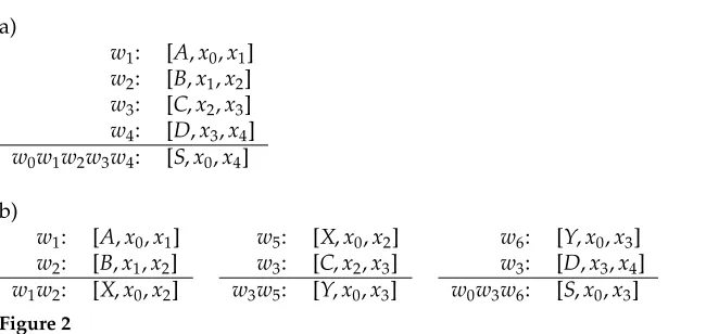
It is often possible to improve the computational complexity of a deduction rule by decomposing the computation into two or more new rules, each having a smaller number of variables than the original rule. We refer to this process asfactorization. One straightforward example of rule factorization is the binarization of a CFG, as shown in Figure 2. Given a deduction rule for a CFG rule withrnonterminals on the righthand side, and a total ofr+1 variables, an equivalent set of rules can be produced, each with three variables, storing intermediate results that indicate that a substring of the original rule’s righthand side has been recognized. This type of rule factorization produces an O(n3) parser for any input CFG.

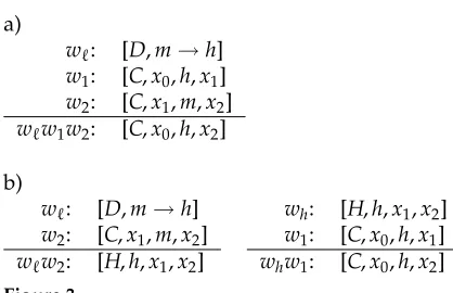
Another well-known instance of rule factorization is the hook trick of Eisner and Satta (1999), which reduces the complexity of parsing for bilexicalized CFGs from O(n5) toO(n4). The basic rule for bilexicalized parsing combines two CFG constituents marked with lexical heads as shown in Figure 3a. Here items with type C indicate constituents, with [C,x0,h,x1] indicating a constituent extending from position x0 to

positionx1, headed by the word at positionh. The item [D,m→h] is used to indicate

the weight assigned by the grammar to a bilexical dependency headed by the word at

a)

w1: [A,x0,x1]

w₂: [B,x₁,x₂] w₃: [C,x₂,x₃] w₄: [D,x₃,x₄] w0w1w2w3w4: [S,x0,x4]

b)

w1: [A,x0,x1]

w2: [B,x1,x2]

w1w2: [X,x0,x2]

w5: [X,x0,x2]

w3: [C,x2,x3]

w3w5: [Y,x0,x3]

w6: [Y,x0,x3]

w3: [D,x3,x4]

w0w3w6: [S,x0,x3]

Figure 2

a)

w: [D,m→h]

w1: [C,x0,h,x1]

w2: [C,x1,m,x2]

ww1w2: [C,x0,h,x2]

b)

w: [D,m→h]

w2: [C,x1,m,x2]

ww2: [H,h,x1,x2]

wh: [H,h,x1,x2]

w1: [C,x0,h,x1]

w_hw₁: [C,x₀,h,x₂] Figure 3

Rule factorization for bilexicalized parsing.

positionhwith the word at positionmas a modifier. The deduction rule is broken into two steps, one which includes the weight for the bilexical grammar rule, and another which identifies the boundaries of the new constituent, as shown in Figure 3b. The hook trick has also been applied to Tree Adjoining Grammar (TAG; Eisner and Satta 2000), and has been generalized to improve the complexity of machine translation decoding under synchronous context-free grammars (SCFGs) with an n-gram language model (Huang, Zhang, and Gildea 2005).

Rule factorization has also been studied in the context of parsing for SCFGs. Unlike monolingual CFGs, SCFGs cannot always be binarized; depending on the permutation between nonterminals in the two languages, it may or may not be possible to reduce the rank, or number of nonterminals on the righthand side, of a rule. Algorithms for finding the optimal rank reduction of a specific rule are given by Zhang and Gildea (2007). The complexity of synchronous parsing for a rule of rank risO(n2r+2), so reducing rank improves parsing complexity.

Rule factorization has also been applied to Linear Context-Free Rewriting Systems (LCFRS), which generalize CFG, TAG, and SCFG to define a rewriting system where nonterminals may have arbitrary fan-out, which indicates the number of continuous spans that a nonterminal accounts for in the string (Vijay-Shankar, Weir, and Joshi 1987). Recent work has examined the problem of factorization of LCFRS rules in order to reduce rank without increasing grammar fan-out (G ´omez-Rodr´ıguez et al. 2009), as well as factorization with the goal of directly minimizing the parsing complexity of the new grammar (Gildea 2010).

We define factorization as a process which applies to rules of the input grammar independently. Individual rules are replaced with an equivalent set of new rules, which must derive the same set of consequent items as the original rule given the same an-tecedent items. While new intermediate items of distinct types may be produced, the set of items and weights derived by the original weighted deduction system is unchanged. This definition of factorization is broad enough to include all of the previous examples, but does not include, for example, the fold/unfold operation applied to grammars by Johnson (2007) and Eisner and Blatz (2007). Rule factorization corresponds to the unfold operation of fold/unfold.

grammar transformations, no general algorithms are known for identifying an optimal series of transformations in this setting. Considering input rules independently allows us to provide algorithms for optimal factorization.

In this article, we wish to provide a general framework for factorization of deduc-tive parsing systems in order to minimize computational complexity. We show how to apply the graph-theoretic property of treewidth to the factorization problem, and examine the question of whether efficient algorithms exist for optimizing the parsing complexity of general parsing systems in this framework. In particular, we show that the existence of a polynomial time algorithm for optimizing the parsing complexity of general LCFRS rules would imply an improved approximation algorithm for the well-studied problem of treewidth of general graphs.

2. Treewidth and Rule Factorization

In this section, we introduce the graph-theoretic property known as treewidth, and show how it can be applied to rule factorization.

Atree decompositionof a graphG=(V,E) is a type of tree having a subset ofG’s vertices at each node. We define the nodes of this treeT to be the setI, and its edges to be the setF. The subset ofV associated with node iof T is denoted byXi. A tree

decomposition is therefore defined as a pair ({Xi|i∈I},T=(I,F)) where eachXi,i∈I

is a subset ofV, and treeThas the following properties:

r

i∈IXi=V.

r

r

Xk⊆Xj.

The treewidth of a tree decomposition ({Xi},T) is maxi|Xi| −1. The treewidth of a

graph is the minimum treewidth over all tree decompositions:

tw(G)= min

({Xi},T)∈TD(G)

max

i |

Xi| −1

whereTD(G) is the set of valid tree decompositions ofG. We refer to a tree decomposi-tion achieving the minimum possible treewidth as being optimal.

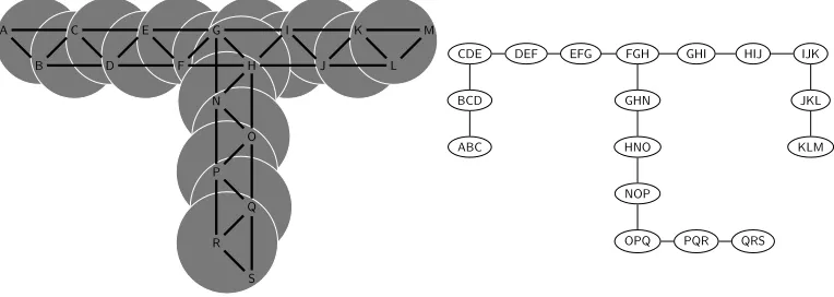
Figure 4

A tree decomposition of a graph is a set of overlapping clusters of the graph’s vertices, arranged in a tree. This example has treewidth = 2.

We can factorize a deduction rule by representing the rule as a graph, which we call adependency graph, and searching for tree decompositions of this graph. For a rulerhavingnvariablesV={vi|i∈ {1,. . .,n}},mantecedent itemsAi,i∈ {1,. . .,m},

and consequentC, letV(Ai)⊂Vbe the variables appearing in antecedentAi, andV(C)

be the variables appearing in the consequent. The dependency graph representation of the rule isGr=(V,E=

S:A1,...,Am,C{(vi,vj)|vi,vj∈V(S)}). That is, we have a vertex for

each variable in the rule, and connect any two vertices that appear together in the same antecedent, or that appear together in the consequent.

The dependency graph representation allows us to prove the following result con-cerning parsing complexity:

Theorem 1

Given a deduction rulerfor parsing where the input string is referenced only through position variables appearing as arguments of antecedent and consequent items, the opti-mal complexity of any factorization of rulerisO(ntw(Gr)+1_{), whereG}

ris the dependency

graph derived fromr.

Proof

One consequence of the definition of a tree decomposition is that, for any clique appear-ing in the original graphG_r, there must exist a node in the tree decompositionTwhich contains all the vertices in the clique. We use this fact to show that there is a one-to-one correspondence between tree decompositions of a rule’s dependency graphGrand

factorizations of the rule.

First, we need to show that any tree decomposition ofGrcan be used as a

factoriza-tion of the original deducfactoriza-tion rule. By our earlier definifactoriza-tion, a factorizafactoriza-tion must derive the same set of consequent items from a given set of antecedent items as the original rule. BecauseGrincludes a clique connecting all variables in the consequentC, the tree

decompositionTmust have a nodeXcsuch thatV(C)⊆Xc. We consider this node to be

the root ofT. The original deduction rule can be factorized into a new set of rules, one for each node inT. For nodeXc, the factorized rule hasCas a consequent, and all other

nodesXihave a new partial result as a consequent, consisting of the variablesXi∩Xj,

whereXjisXi’s neighbor on the path to the root nodeXc. We must guarantee that the

over all variable values of the semiring product of the antecedents’ weights. The tree structure ofTcorresponds to a factorization of this semiring expression. For example, if we represent the CFG rule of Figure 2a with the generalized semiring expression:

x1x2x3

A(x0,x1)⊗B(x1,x2)⊗C(x2,x3)⊗D(x3,x4)

the factorization of this expression corresponding to the binarized rule is

x3

x2

x1

A(x0,x1)⊗B(x1,x2)

⊗C(x2,x3)

⊗D(x3,x4)

where semiring operations⊕and⊗have been interchanged as allowed by the depen-dency graph for this rule.

Because each antecedent Ai is represented by a clique in the graph Gr, the tree

decomposition T must contain at least one node which includes all variablesV(Ai).

We can choose one such node and multiply in the weight of Ai, given the values of

variablesV(Ai), at this step of the expression. The running intersection property of the

tree decomposition guarantees that each variable has a consistent value at each point where it is referenced in the factorization.

The same properties guarantee that any valid rule factorization corresponds to a tree decomposition of the graphG_r. We consider the tree decomposition with a setX_i for each new ruleri, consisting of all variables used inri, and with tree edgesTdefined

by the producer/consumer relation over intermediate results in the rule factorization. Each antecedent of the original rule must appear in some new rule in the factorization, as must the consequent of the original rule. Therefore, all edges in the original rule’s dependency graphGr appear in some tree nodeXi. Any variable that appears in two

rules in the factorization must appear in all intermediate rules in order to ensure that the variable has a consistent value in all rules that reference it. This guarantees the running intersection property of the tree decomposition ({Xi},T). Thus any rule factorization,

when viewed as a tree of sets of variables, has the properties that make it a valid tree decomposition ofGr.

The theorem follows as a consequence of the one-to-one correspondence between rule factorizations and tree decompositions.

2.1 Computational Complexity

Factorization produces, for each input rule havingmantecedents, at mostm−1 new rules, each containing at most the same number of nonterminals and the same number of variables as the input rule. Hence, the size of the new factorized grammar isO(|G|2), and we avoid any possibility of an exponential increase in grammar size. Tighter bounds can be achieved for specific classes of input grammars.

extracted from word-aligned bitext (Wellington, Waxmonsky, and Melamed 2006; Huang et al. 2009) or from dependency treebanks (Kuhlmann and Nivre 2006; Gildea 2010). In this setting, the rules having treewidthkcan be identified in timeO(k+2) using the simple algorithm of Arnborg, Corneil, and Proskurowski (1987), (where again is the number of variables in the input rules), or in timeO() using the algorithm of Bodlaender (1996).

2.2 Cyclic Dependencies

Although this article primarily addresses the case where there are no cyclic dependen-cies between rule instantiations, we note here that our techniques carry over to the cyclic case under certain conditions. If there are cycles in the rule dependencies, but the semiring meets Knuth’s (1977) definition of asuperiorfunction, parsing takes time O(MlogM), whereM is the number of rule instantiations, and the extra logM term accounts for maintaining an agenda as a priority queue (Nederhof 2003). Cycles in the rule dependencies may arise, for example, from chains of unary productions in a CFG; the properties of superior functions guarantee that unbounded chains need not be considered. The max-product semiring used in Viterbi parsing has this property, assuming that all rule weights are less than one, whereas for exact computation with the sum-product semiring, unbounded chains must be considered. As in the acyclic case, M=O(nk) for parsing problems where rules have at most k variables. Under the assumption of superior functions, parsing takes time O(nkklogn) with Knuth’s algorithm. In this setting, as in the acyclic case, minimizingkwith tree decomposition minimizes parsing complexity.

2.3Related Applications of Treewidth

The technique of using treewidth to minimize complexity has been applied to constraint satisfaction (Dechter and Pearl 1989), graphical models in machine learning (Jensen, Lauritzen, and Olesen 1990; Shafer and Shenoy 1990), and query optimization for databases (Chekuri and Rajaraman 1997). Our formulation of parsing is most closely related to logic programming; in this area treewidth has been applied to limit complex-ity in settings where either the deduction rules or the input database of ground facts have fixed treewidth (Flum, Frick, and Grohe 2002). Whereas Flum, Frick, and Grohe (2002) apply treewidth to nonrecursive datalog programs, our parsing programs have unbounded recursion, as the depth of the parse tree is not fixed in advance. Our results for parsing can be seen as a consequence of the fact that, even in the case of unbounded recursion, the complexity of (unweighted) datalog programs is linear in the number of possible rule instantiations (McAllester 2002).

3. Examples of Treewidth for Parsing

In this section, we show how a few well-known parsing algorithms can be derived automatically by finding the optimal tree decomposition of a dependency graph.

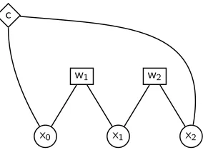
Figure 5

Factor graph for the binary CFG deduction rule of Figure 1.

consequent nodes are a new feature of this representation. We can think of consequents as factors with weight = 1; they do not affect the weights computed, but serve to guarantee that the consequent of the original rule can be found in one node of the tree decomposition. We refer to both antecedent and consequent nodes as factor nodes. Re-placing each factor node with a clique over its neighbor variables yields the dependency graphGrdefined earlier. We represent variables with circles, antecedents with squares

labeled with the antecedent’s weight, and consequents with diamonds labeled c. An example factor graph for the simple CFG rule of Figure 1 is shown in Figure 5.

3.1 CFG Binarization

Figure 6a shows the factor graph derived from the monolingual CFG rule with four children in Figure 2a. The dependency graph obtained by replacing each factor with a clique of size 2 (a single edge) is a graph with one large cycle, shown in Figure 6b. Finding the optimal tree decomposition yields a tree with nodes of size 3,{x₀,x_i,x_i+1} for eachi, shown in Figure 6c. Each node in this tree decomposition corresponds to one of the factored deduction rules in Figure 2b. Thus, the tree decomposition shows us how

Figure 6

to parse in timeO(n3); finding the tree decomposition of a long CFG rule is essentially equivalent to converting to Chomsky Normal Form.

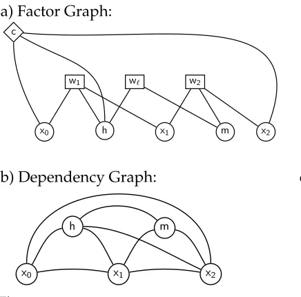
3.2 The Hook Trick

The deduction rule for bilexicalized parsing shown in Figure 3a translates into the factor graph shown in Figure 7a. Factor nodes are created for the two existing constituents from the chart, with the first extending from position x₀ in the string tox₁, and the second from x1 to x2. Both factor nodes are connected not only to the start and end

points, but also to the constituent’s head word, h for the first constituent and mfor the second (we show the construction of a left-headed constituent in the figure). An additional factor is connected only tohandmto represent the bilexicalized rule weight, expressed as a function of h and m, which is multiplied with the weight of the two existing constituents to derive the weight of the new constituent. The new constituent is represented by a consequent node at the top of the graph—the variables that will be relevant for its further combination with other constituents are its end pointsx0andx2

and its head wordh.

Placing an edge between each pair of variable nodes that share a factor, we get Fig-ure 7b. If we compute the optimal tree decomposition for this graph, shown in FigFig-ure 7c, each of the two nodes corresponds to one of the factored rules in Figure 3b. The largest node of the tree decomposition has four variables, giving theO(n4) algorithm of Eisner and Satta (1999).

3.3 SCFG Parsing Strategies

SCFGs generalize CFGs to generate two strings with isomorphic hierarchical structure simultaneously, and have become widely used as statistical models of machine transla-tion (Galley et al. 2004; Chiang 2007). We write SCFG rules as productransla-tions with one

Figure 7

lefthand side nonterminal and two righthand side strings. Nonterminals in the two strings are linked with superscript indices; symbols with the same index must be further rewritten synchronously. For example,

X→A(1)B(2)C(3)D(4), A(1)B(2)C(3)D(4) (1)

is a rule with four children and no reordering, whereas

X→A(1)B(2)C(3)D(4), B(2)D(4)A(1)C(3) (2)

expresses a more complex reordering. In general, we can take indices in the first righthand-side string to be consecutive, and associate a permutationπwith the second string. If we use Xi for 0≤i≤n as a set of variables over nonterminal symbols (for

example,X₁andX₂may both stand for nonterminalA), we can write rules in the general form:

X0 →X (1) 1 · · ·X

(n) n , X

(π(1))

π(1) · · ·X (π(n))

π(n)

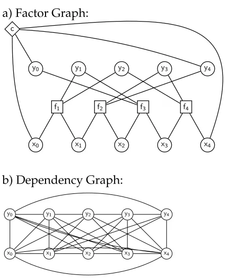
Unlike monolingual CFGs, SCFGs cannot always be binarized. In fact, the lan-guages of string pairs generated by a synchronous grammar can be arranged in an infinite hierarchy, with each rank≥4 producing languages not possible with grammars restricted to smaller rules (Aho and Ullman 1972). For any grammar with maximum rank r, converting each rule into a single deduction rule yields an O(n2r+2) parsing algorithm, because there arer+1 boundary variables in each language. More efficient parsing algorithms are often possible for specific permutations, and, by Theorem 1, the best algorithm for a permutation can be found by computing the minimum-treewidth tree decomposition of the graph derived from the SCFG deduction rule for a specific permutation. For example, for the non-binarizable rule of Equation (2), the resulting factor graph is shown in Figure 8a, where variablesx0,. . .,x4indicate position variables

in one language of the synchronous grammar, andy0,. . .,y4 are positions in the other

language. The optimal tree decomposition for this rule is shown in Figure 8c. For this permutation, the optimal parsing algorithm takes timeO(n8), because the largest node in the tree decomposition of Figure 8c includes eight position variables. This result is intermediate between theO(n6) for binarizable SCFGs, also known as Inversion Trans-duction Grammars (Wu 1997), and theO(n10) that we would achieve by recognizing the rule in a single deduction step.

Gildea and ˇStefankoviˇc (2007) use a combinatorial argument to show that as the number of nonterminals r in an SCFG rule grows, the parsing complexity grows as

Ω(ncr) for some constantc. In other words, some very difficult permutations exist of all lengths.

Figure 8

Treewidth applied to the SCFG rule of Equation (2).

4. LCFRS Parsing Strategies

LCFRS provides a generalization of a number of widely used formalisms in natural language processing, including CFG, TAG, SCFG, and synchronous TAG. LCFRS has also been used to model non-projective dependency grammars, and the LCFRS rules extracted from dependency treebanks can be quite complex (Kuhlmann and Satta 2009), making factorization important. Similarly, LCFRS can model translation relations beyond the power of SCFG (Melamed, Satta, and Wellington 2004), and grammars extracted from word-aligned bilingual corpora can also be quite complex (Wellington, Waxmonsky, and Melamed 2006). An algorithm for factorization of LCFRS rules is presented by Gildea (2010), exploiting specific properties of LCFRS. The tree decompo-sition method achieves the same results without requiring analysis specific to LCFRS. In this section, we examine the complexity of rule factorization for general LCFRS grammars.

An LCFRS is defined as a tuple G=(VT,VN,P,S), where VT is a set of terminal

symbols,VN is a set of nonterminal symbols,Pis a set of productions, andS∈VN is a

distinguished start symbol. Associated with each nonterminalBis a fan-outϕ(B), which tells how many continuous spansBcovers. Productionsp∈Ptake the form:

p:A→g(B1,B2,. . .,Br) (3)

whereA,B1,. . .,Br∈VN, andgis a function

g: (V∗_T)ϕ(B1)× · · · ×_(V∗ T)

ϕ(Br)→_(V∗

T)

ϕ(A)

which specifies how to assemble ther_i=1ϕ(Bi) spans of the righthand side

nontermi-nals into theϕ(A) spans of the lefthand side nonterminal. The functiongmust belinear

andnon-erasing, which means that if we write

g(s1,1,. . .,s1,ϕ(B1),. . .,s1,1,. . .,s1,ϕ(Br))=t1,. . .,tϕ(A)

the tuple of stringst1,. . .,tϕ(A)on the righthand side contains each variablesi,jfrom

the lefthand side exactly once, and may also contain terminals fromVT. The process of

generating a string from an LCFRS grammar can be thought of as first choosing, top-down, a production to expand each nonterminal, and then, bottom–up, applying the functions associated with each production to build the string. As an example, the CFG

S→A B

A→a

B→b

corresponds to the following grammar in LCFRS notation:

S→gS(A,B) gS(sA,sB)=sAsB

A→gA() gA()=a

B→g_B() g_B()=b

Here, all nonterminals have fan-out = 1, reflected in the fact that all tuples defining the productions’ functions contain just one string. As CFG is equivalent to LCFRS with fan-out = 1, SCFG and TAG can be represented as LCFRS with fan-fan-out = 2. Higher values of fan-out allow strictly more powerful grammars (Rambow and Satta 1999). Polynomial-time parsing is possible for any fixed LCFRS grammar, but the degree of the polynomial depends on the grammar. Parsing general LCFRS grammars, where the grammar is considered part of the input, is NP-complete (Satta 1992).

4.1 Graphs Derived from LCFRS Rules

variable will occur exactly twice in the deduction rule: either in two antecedents, if two nonterminals on the rule’s righthand side are adjacent, or once in an antecedent and once in the consequent, if the variable indicates a boundary of any segment of the rule’s lefthand side.

Converting such deduction rules into dependency graphs, we see that the cliques of the dependency graph may be arbitrarily large, due to the unbounded fan-out of LCFRS nonterminals. However, each vertex appears in only two cliques, because each boundary variable in the rule is shared by exactly two nonterminals. In the remainder of this section, we consider whether the problem of finding the optimal tree decomposition of this restricted set of graphs is also NP-complete, or whether efficient algorithms may be possible in the LCFRS setting.

4.2 Approximation of Treewidth for General Graphs

We will show that an efficient algorithm for finding the factorization of an arbitrary LCFRS production that optimizes parsing complexity would imply the existence of an algorithm for treewidth that returns a result within a factor of 4∆(G) of the optimum, where∆(G) is the maximum degree of the input graph. Although such an approxima-tion algorithm may be possible, it would require progress in fundamental problems in graph theory.

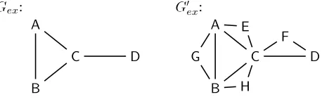
Consider an arbitrary graphG=(V,E), and definekto be its treewidth,k=tw(G). We wish to construct a new graph G=(V,E) fromG in such a way that tw(G)=

tw(G) and every vertex inGhas even degree. This can be accomplished by doubling the graph’s edges in the manner shown in Figure 9. To double the edges, for every edge e=(u,v) inE, we add a new vertex ˆetoGand add edges (u, ˆe) and (v, ˆe) toG. We also include every edge in the original graphGinG. Now, every vertexvinGhas degree = 2, if it is a newly created vertex, or twice the degree ofvinGotherwise, and therefore

∆(G)=2∆(G) (4)

We now show thattw(G)=tw(G), under the assumption thattw(G)≥3. Any tree decomposition of Gcan be adapted to a tree decomposition of G by adding a node containing{u,v, ˆe}for each edgeein the original graph, as shown in Figure 10. The new node can be attached to a node containinguandv; because uandvare connected by an edge inG, such a node must exist inG’s tree decomposition. The vertex ˆewill not occur anywhere else in the tree decomposition, and the occurrences ofuandvstill form a connected subtree. For each edgee=(u,v) inG, the tree decomposition must have a node containinguandv; this is the case because, ifeis an original edge fromG, there is already a node in the tree decomposition containinguandv, whereas ifeis an edge to a newly added vertex inG, one of the newly added nodes in the tree decomposition

Figure 9

Figure 10

Tree decompositions ofGexandGex.

will contain its endpoints. We constructed the new tree decomposition by adding nodes of size 3. Therefore, as long as the treewidth of Gwas at least 3, tw(G)≤tw(G). In the other direction, becauseGis a subgraph ofG, any tree decomposition ofGforms a valid tree decomposition ofGafter removing the vertices inG−G, and hencetw(G)≥

tw(G). Therefore,

tw(G)=tw(G) (5)

Because every vertex in G has even degree, G has an Eulerian tour, that is, a path visiting every edge exactly once, beginning and ending at the same vertex. Let π=π₁,. . .,π_nbe the sequence of vertices along such a tour, withπ₁ =π_n. Note that the sequence π contains repeated elements. Let µ_i,i∈ {1,. . .,n} indicate how many times we have visited π_i on the ith step of the tour: µ_i=|{j|π_j=π_i,j∈ {1,. . .,i}}|. We now construct an LCFRS productionPwith|V|righthand side nonterminals from the Eulerian tour:

P:X→g(B₁,. . .,B_|V|)

g(s_1,1,. . .,s_1,φ(B1),. . .,s|V|,1,. . .,s|V|,φ(B_|V|))=sπ1,µ1· · ·sπn,µn

The fan-outφ(B_i) of each nonterminalB_iis the number of times vertexiis visited on the Eulerian tour. The fan-out of the lefthand side nonterminalXis one, and the lefthand side is constructed by concatenating the spans of each nonterminal in the order specified by the Eulerian tour.

For the example graph in Figure 9, one valid tour is

π_ex=A,B,C,D,F,C,E,A,G,B,H,C,A

This tour results in the following LCFRS production:

Pex:X→gex(A,B,C,D,E,F,G,H)

gex(sA,1,sA,2,sA,3,sB,1,sB,2,sC,1,sC,2,sC,3,sD,1,sE,1,sF,1,sG,1,sH,1)= sA,1sB,1sC,1sD,1sF,1sC,2sE,1sA,2sG,1sB,2sH,1sC,3sA,3

end points of the nonterminals inP. The edges inGare formed by adding a clique for each nonterminal inP connecting all its beginning and end points, that is,2₂fedges for a nonterminal of fan-out f. We must include a clique for X, the lefthand side of the production. However, because the righthand side of the production begins and ends with the same nonterminal, the vertices for the beginning and end points of X are already connected, so the lefthand side does not affect the graph structure for the entire production. By Theorem 1, the optimal parsing complexity ofPistw(G)+1.

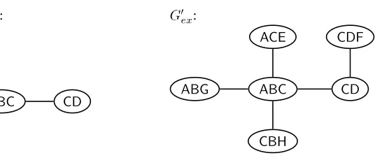
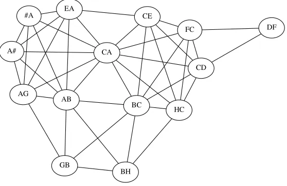
The graphs G and G are related in the following manner: Every edge in G corresponds to a vertex inG, and every vertex in G corresponds to a clique in G. We can identify vertices inGwith unordered pairs of vertices{u,v}inG. The edges in Gare ({u,v},{u,w})∀u,v,w:u=v,u=w,v=w. An example ofGderived from our example productionPexis shown in Figure 11.

Any tree decompositionTofG can be transformed into a valid tree decomposi-tionTofGby simply replacing each vertex in each node ofTwith both corresponding vertices inG. IfTwitnesses a tree decomposition of optimal widthk=tw(G), each node in T will produce a node of size at most 2k inT. For any vertexvinG, one node inTmust contain the clique corresponding tovinG. Each vertex{v,w}inG must be found in a contiguous subtree of T, and these subtrees all include the node containing the clique forv. The occurrences ofvinTare the union of these contiguous subtrees, which must itself form a contiguous subtree. Furthermore, each edge (u,v) in Gcorresponds to some vertex inG, souandvmust occur together in some node of T. Combining these two properties, we see thatTis a valid tree decomposition ofG. From the construction, ifSOLis the treewidth ofT, we are guaranteed that

SOL≤2tw(G) (6)

In the other direction, any tree decomposition T ofGcan be transformed into a tree decompositionTofGby simply replacing each occurrence of vertexvin a node ofTwith all vertices{v,w}inT. The number of such vertices is the degree ofv,∆(v).

Figure 11

Each vertex {v,w}occurs in a contiguous subtree ofT becausev andwoccurred in contiguous subtrees of T, and had to co-occur in at least one node of T. Each edge inG comes from a clique for some vertexvinG, so the edge has both its endpoints in any node ofTcorresponding to a node ofTthat containedv. ThusTis a valid tree decomposition ofG. We expand each node in the tree decomposition by at most the maximum degree of the graph∆(G), and therefore

tw(G)≤∆(G)tw(G) (7)

Assume that we have an efficient algorithm for computing the optimal parsing strategy of an arbitrary LCFRS rule. Consider the following algorithm for finding a tree decomposition of an input graphG:

r

r

r

map this into a tree decomposition ofG, and then remove all new nodes ˆe to obtain a tree decomposition ofGof treewidthSOL.

Iftw(G)=k, we haveSOL≤2k from Equation (6), andk≤∆(G)tw(G) from Equation (7). Putting these together:

SOL≤2∆(G)tw(G)

and using Equations (4) and (5) to relate our result to the original graphG,

SOL≤4∆(G)tw(G)

This last inequality proves the main result of this section

Theorem 2

An algorithm for finding the optimal parsing strategy of an arbitrary LCFRS production would imply a 4∆(G) approximation algorithm for treewidth.

Whether such an approximation algorithm for treewidth is possible is an open prob-lem. The best-known result is theO( logk) approximation result of Feige, Hajiaghayi, and Lee (2005), which improves on theO(logk) result of Amir (2001). This indicates that, although polynomial-time factorization of LCFRS rules to optimize parsing complexity may be possible, it would require progress on general algorithms for treewidth.

5. Conclusion

typically small, and finding the tree decomposition is not computationally expensive, and in fact is trivial in comparison to the original parsing problem. Given the special structure of the graphs derived from LCFRS productions, however, we have explored whether finding optimal tree decompositions of these graphs, and therefore optimal parsing strategies for LCFRS productions, is also NP-complete. Although a polynomial time algorithm for this problem would not necessarily imply that P=NP, it would require progress on fundamental, well-studied problems in graph theory. Therefore, it does not seem possible to exploit the special structure of graphs derived from LCFRS productions.

Acknowledgments

This work was funded by NSF grants IIS-0546554 and IIS-0910611. We are grateful to Giorgio Satta for extensive discussions on grammar factorization, as well as for

feedback on earlier drafts from Mehdi Hafezi Manshadi, Matt Post, and four anonymous reviewers.

References

Aho, Albert V. and Jeffery D. Ullman. 1972. The Theory of Parsing, Translation, and Compiling, volume 1. Prentice-Hall, Englewood Cliffs, NJ.

Amir, Eyal. 2001. Efficient approximation for triangulation of minimum treewidth. In17th Conference on Uncertainty in Artificial Intelligence, pages 7–15, Seattle, WA.

Arnborg, Stefen, Derek G. Corneil, and Andrzej Proskurowski. 1987. Complexity of finding embeddings in ak-tree.SIAM Journal of Algebraic and Discrete Methods, 8:277–284.

Bar-Hillel, Yehoshua, M. Perles, and E. Shamir. 1961. On formal properties of simple phrase structure grammars. Zeitschrift f ¨ur Phonetik, Sprachwissenschaft und Kommunikationsforschung, 14:143–172. Reprinted in Y. Bar-Hillel. (1964).Language and Information: Selected Essays on Their Theory and Application, Addison-Wesley Reading, MA, pages 116–150.

Bodlaender, H. L. 1996. A linear time algorithm for finding tree decompositions of small treewidth.SIAM Journal on Computing, 25:1305–1317.

Bodlaender, Hans L., John R. Gilbert, Hj ´almt ´yr Hafsteinsson, and Ton Kloks. 1995. Approximating treewidth, pathwidth, frontsize, and shortest elimination tree.Journal of Algorithms, 18(2):238–255.

Chekuri, Chandra and Anand Rajaraman. 1997. Conjunctive query containment revisited. InDatabase Theory – ICDT ’97,

volume 1186 ofLecture Notes in Computer Science. Springer, Berlin, pages 56–70. Chiang, David. 2007. Hierarchical

phrase-based translation.Computational Linguistics, 33(2):201–228.

Dechter, Rina and Judea Pearl. 1989. Tree clustering for constraint networks. Artificial Intelligence, 38(3):353–366. Eisner, Jason and John Blatz. 2007. Program

transformations for optimization of parsing algorithms and other weighted logic programs. In Shuly Wintner, editor, Proceedings of FG 2006: The 11th Conference on Formal Grammar. CSLI Publications, pages 45–85, Malaga.

Eisner, Jason and Giorgio Satta. 1999. Efficient parsing for bilexical context-free grammars and head automaton grammars. InProceedings of the 37th Annual Conference of the Association for Computational Linguistics (ACL-99), pages 457–464, College Park, MD.

Eisner, Jason and Giorgio Satta. 2000. A faster parsing algorithm for lexicalized

tree-adjoining grammars. InProceedings of the 5th Workshop on Tree-Adjoining

Grammars and Related Formalisms (TAG+5), pages 14–19, Paris.

Feige, Uriel, MohammadTaghi Hajiaghayi, and James R. Lee. 2005. Improved approximation algorithms for

minimum-weight vertex separators. In STOC ’05: Proceedings of the thirty-seventh annual ACM symposium on Theory of computing, pages 563–572, Baltimore, MD. Flum, J ¨org, Markus Frick, and Martin Grohe.

2002. Query evaluation via

tree-decompositions.Journal of the ACM, 49(6):716–752.

Galley, Michel, Mark Hopkins, Kevin Knight, and Daniel Marcu. 2004. What’s in a translation rule? InProceedings of the 2004 Meeting of the North American Chapter of the Association for Computational Linguistics (NAACL-04), pages 273–280, Boston, MA. Gildea, Daniel. 2010. Optimal parsing

Rewriting Systems. InProceedings of the 2010 Meeting of the North American Chapter of the Association for Computational Linguistics (NAACL-10), pages 769–776, Los Angeles, CA.

Gildea, Daniel and Daniel ˇStefankoviˇc. 2007. Worst-case synchronous grammar rules. In Proceedings of the 2007 Meeting of the North American Chapter of the Association for Computational Linguistics (NAACL-07), pages 147–154, Rochester, NY. G ´omez-Rodr´ıguez, Carlos, Marco

Kuhlmann, Giorgio Satta, and David Weir. 2009. Optimal reduction of rule length in Linear Context-Free Rewriting Systems. In Proceedings of the 2009 Meeting of the North American Chapter of the Association for Computational Linguistics (NAACL-09), pages 539–547, Boulder, CO.

Goodman, Joshua. 1999. Semiring parsing. Computational Linguistics, 25(4):573–605. Huang, Liang, Hao Zhang, and Daniel

Gildea. 2005. Machine translation as lexicalized parsing with hooks. In International Workshop on Parsing Technologies (IWPT05), pages 65–73, Vancouver.

Huang, Liang, Hao Zhang, Daniel Gildea, and Kevin Knight. 2009. Binarization of synchronous context-free grammars. Computational Linguistics, 35(4):559–595. Jensen, Finn V., Steffen L. Lauritzen, and

Kristian G. Olesen. 1990. Bayesian updating in causal probabilistic networks by local computations.Computational Statistics Quarterly, 4:269–282. Johnson, Mark. 2007. Transforming

projective bilexical dependency grammars into efficiently-parsable CFGs with unfold-fold. InProceedings of the 45th Annual Meeting of the Association of Computational Linguistics, pages 168–175, Prague.

Knuth, D. 1977. A generalization of Dijkstra’s algorithm.Information Processing Letters, 6(1):1–5.

Kschischang, F. R., B. J. Frey, and H. A. Loeliger. 2001. Factor graphs and the sum-product algorithm.IEEE Transactions on Information Theory, 47(2):498–519. Kuhlmann, Marco and Joakim Nivre. 2006.

Mildly non-projective dependency structures. InProceedings of the International Conference on Computational

Linguistics/Association for Computational Linguistics (COLING/ACL-06),

pages 507–514, Sydney.

Kuhlmann, Marco and Giorgio Satta. 2009. Treebank grammar techniques for

non-projective dependency parsing. In Proceedings of the 12th Conference of the European Chapter of the ACL (EACL-09), pages 478–486, Athens.

McAllester, David. 2002. On the complexity analysis of static analyses.Journal of the ACM, 49(4):512–537.

Melamed, I. Dan, Giorgio Satta, and Ben Wellington. 2004. Generalized multitext grammars. InProceedings of the 42nd Annual Conference of the Association for Computational Linguistics (ACL-04), pages 661–668, Barcelona.

Nederhof, M.-J. 2003. Weighted deductive parsing and Knuth’s algorithm. Computational Linguistics, 29(1):135–144. Rambow, Owen and Giorgio Satta. 1999.

Independent parallelism in finite copying parallel rewriting systems. Theoretical Computer Science, 223(1-2):87–120.

Satta, Giorgio. 1992. Recognition of Linear Context-Free Rewriting Systems. In Proceedings of the 30th Annual Conference of the Association for Computational Linguistics (ACL-92), pages 89–95, Newark, DE. Shafer, G. and P. Shenoy. 1990. Probability

propagation.Annals of Mathematics and Artificial Intelligence, 2:327–353. Shieber, Stuart M., Yves Schabes, and

Fernando C. N. Pereira. 1995. Principles and implementation of deductive parsing. The Journal of Logic Programming,

24(1-2):3–36.

Vijay-Shankar, K., D. L. Weir, and A. K. Joshi. 1987. Characterizing structural

descriptions produced by various grammatical formalisms. InProceedings of the 25th Annual Conference of the Association for Computational Linguistics (ACL-87), pages 104–111, Stanford, CA.

Wellington, Benjamin, Sonjia Waxmonsky, and I. Dan Melamed. 2006. Empirical lower bounds on the complexity of translational equivalence. InProceedings of the International Conference on Computational Linguistics/Association for Computational Linguistics (COLING/ACL-06),

pages 977–984, Sydney.

Wu, Dekai. 1997. Stochastic inversion transduction grammars and bilingual parsing of parallel corpora.Computational Linguistics, 23(3):377–403.