Speculation and Negation: Rules, Rankers, and the Role of Syntax

and the Role of Syntax

Erik Velldal

Lilja Øvrelid

Jonathon Read

Stephan Oepen

This article explores a combination of deep and shallow approaches to the problem of resolving the scope of speculation and negation within a sentence, specifically in the domain of biomedical research literature. The first part of the article focuses on speculation. After first showing how speculation cues can be accurately identified using a very simple classifier informed only by local lexical context, we go on to explore two different syntactic approaches to resolving the in-sentence scopes of these cues. Whereas one uses manually crafted rules operating over depen-dency structures, the other automatically learns a discriminative ranking function over nodes in constituent trees. We provide an in-depth error analysis and discussion of various linguistic properties characterizing the problem, and show that although both approaches perform well in isolation, even better results can be obtained by combining them, yielding the best published results to date on the CoNLL-2010 Shared Task data. The last part of the article describes how our speculation system is ported to also resolve the scope of negation. With only modest modifications to the initial design, the system obtains state-of-the-art results on this task also.

1. Introduction

The task of providing a principled treatment of speculation and negation is a problem that has received increased interest within the NLP community during recent years. This is witnessed not only by this Special Issue, but also by the themes of several recent shared tasks and dedicated workshops. The Shared Task at the 2010 Conference on Nat-ural Language Learning (CoNLL) has been of central importance in this respect, where the topic was speculation detection for the domain of biomedical research literature

∗ University of Oslo, Department of Informatics, PB 1080 Blindern, 0316 Oslo, Norway. E-mail: {erikve,liljao,jread,oe}@ifi.uio.no.

(Farkas et al. 2010). This particular area has been the focus of much current research, triggered by the release of the BioScope corpus (Vincze et al. 2008)—a collection of scientific abstracts, full papers, and clinical reports with manual annotations of words that signal speculation or negation (so-calledcues), as well as of thescopesof these cues within the sentences. The following examples from BioScope illustrate how sentences are annotated with respect to speculation. Cues are here shown using angle brackets, with braces corresponding to their annotated scopes:

(1) {The specific role of the chromodomain isunknown}but chromodomain swapping experiments in Drosophila{suggestthat they{mightbe protein interaction modules}}[18].

(2) These data{indicate thatIL-10 and IL-4 inhibit cytokine production by different mechanisms}.

Negation is annotated in the same way, as shown in the following examples:

(3) Thus, positive autoregulation is{neithera consequencenorthe sole cause of growth arrest}.

(4) Samples of the protein pair space were taken{instead ofconsidering the whole space}as this was more computationally tractable.

In this article we develop several linguistically informed approaches to automati-cally identify cues and resolve their scope within sentences, as in the example annota-tions. Our starting point is the system developed by Velldal, Øvrelid, and Oepen (2010) for the CoNLL-2010 Shared Task challenge. This system implements a two-stage hybrid approach for resolving speculation: First, a binary classifier is applied for identifying cues, and then their in-sentence scope is resolved using a small set of manually defined rules operating on dependency structures.

In the current article we present several important extensions to the initial system design of Velldal, Øvrelid, and Oepen (2010): First, in Section 5, we present a simpli-fied approach to cue classification, greatly reducing the model size and complexity of our Support Vector Machine (SVM) classifier while at the same time giving better accuracy. Then, after reviewing the manually defineddependency-based scope rules (Section 6.1), we show how the scope resolution task can be handled using an alternative approach based on learning adiscriminative ranking functionover subtrees of HPSG-derived constituent trees (Section 6.2). Moreover, by combiningthis empirical ranking approach with the manually defined rules (Section 6.3), we are able to obtain the best published results so far (to the best of our knowledge) on the CoNLL-2010 Shared Task evaluation data. Finally, in Section 7, we show how our speculation system can be ported to also resolve the scope ofnegation. Only requiring modest modifications, the system also obtains state-of-the-art results on this task. Rather than merely presenting the implementation details of the new approaches we develop, we also provide in-depth error analyses and discussion on the linguistic properties of the phenomena of both speculation and negation.

2. Data Sets and Preprocessing

Our experiments center on the biomedical abstracts, full papers, and clinical reports of the BioScope corpus (Vincze et al. 2008). This comprises 20,924 sentences (or other root-level utterances), annotated with respect to both negation and speculation. Some basic descriptive statistics for the data sets are provided in Table 1. We see that roughly 18% of the sentences are annotated as uncertain, and 13% contain negations. Note that, for our speculation experiments, we will be using only the abstracts and the papers for training, corresponding to the official CoNLL-2010 Shared Task training data. Moreover, we will be using the Shared Task version of this data, in which certain annotation errors had been corrected. The Shared Task task organizers also provided a set of newly annotated biomedical articles for evaluation purposes, constituting an additional 5,003 utterances. This latter data set (also detailed in Table 1) will be used for held-out testing of our speculation models. We will be using the following abbreviations when referring to the various parts of the data:BSA(BioScope abstracts),BSP (full papers),BSE(the held-out evaluation data), andBSR(clinical reports). Note that, when we get to thenegation

task we will be using theoriginal version of the BioScope data. Furthermore, as BSE does not annotate negation, we instead follow the experimental set-up of Morante and Daelemans (2009b) for the negation task, reporting 10-fold cross validation on BSA and held-out testing on BSP and BSR.

2.1 Tokenization

The BioScope data (and other data sets in the CoNLL-2010 Shared Task), are provided sentence-segmented only, and otherwise non-tokenized. Unsurprisingly, the GENIA tagger (Tsuruoka et al. 2005) has a central role in our pre-processing set-up. We found that its tokenization rules are not always optimally adapted for the type of text in Bio-Scope, however. For example, GENIA unconditionally introduces token boundaries for some punctuation marks that can also occur token-internally, thus incorrectly splitting tokens like390,926,methlycobamide:CoM, orCa(2+). Conversely, GENIA fails to isolate some kinds of opening single quotes, because the quoting conventions assumed in BioScope differ from those used in the GENIA Corpus, and it mis-tokenizes LA TEX-style n- and m-dashes. On average, one in five sentences in the CoNLL training data

Table 1

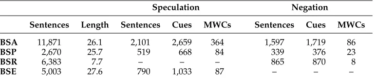
The top three rows summarize the components of the BioScope corpus—abstracts (BSA), full papers (BSP), and clinical reports (BSR)—annotated for speculation and negation. The bottom row details the held-out evaluation data (BSE) provided for the CoNLL-2010 Shared Task. Columns indicate the total number of sentences and their average length, the number of hedged/negated sentences, the number of cues, and the number of multiword cues. (Note that BSE is not annotated for negation, and we do not provide speculation statistics for BSR as this data set will only be used for the negation experiments.

Speculation Negation

Sentences Length Sentences Cues MWCs Sentences Cues MWCs

BSA 11,871 26.1 2,101 2,659 364 1,597 1,719 86

BSP 2,670 25.7 519 668 84 339 376 23

BSR 6,383 7.7 – – – 865 870 8

exhibited GENIA tokenization problems. Our pre-processing approach thus deploys a cascaded finite-state tokenizer (borrowed and adapted from the open-source English Resource Grammar: Flickinger [2002]), which aims to implement the tokenization deci-sions made in the Penn Treebank (Marcus, Santorini, and Marcinkiewicz 1993)—much like GENIA, in principle—but more appropriately treating corner cases like the ones noted here.

2.2 PoS Tagging and Lemmatization

For part-of-speech (PoS) tagging and lemmatization, we combine GENIA (with its built-in, occasionally deviant tokenizer) and TnT (Brants 2000), which operates on pre-tokenized inputs but in its default model is trained on financial news from the Penn Treebank. Our general goal here is to take advantage of the higher PoS accuracy provided by GENIA in the biomedical domain, while using our improved tokenization and producing inputs to the parsers that as much as possible resemble the conventions used in the original training data for the (dependency) parser (the Penn Treebank, once again).

To this effect, for the vast majority of tokens we can align the GENIA tokeniza-tion with our own, and in these cases we typically use GENIA PoS tags and lemmas (i.e., base-forms). For better normalization, we downcase all lemmas except for proper nouns. GENIA does not make a PoS distinction between proper vs. common nouns (as assumed in the Penn Treebank), however, and hence we give precedence to TnT outputs for tokens tagged as nominal by both taggers. Finally, for the small number of cases where we cannot establish a one-to-one correspondence between GENIA tokens and our own tokenization, we rely on TnT annotation only.

2.3 A Methodological Caveat

Unsurprisingly, the majority of previous work on BioScope seems to incorporate infor-mation from the GENIA tagger in one way or another, whether it regards tokenization, lemmatization, PoS information, or named entity chunking. Using the GENIA tagger for pre-processing introduces certain dependencies to be aware of, however, as the abstracts in BioScope are in fact also part of the GENIA corpus (Collier et al. 1999) on which the GENIA tagger is trained. This means that the accuracy of the information provided by the tagger on this subset of BioScope cannot be expected to be representative of the accuracy on other texts. Moreover, this effect might of course also carry over to any downstream components using this information.

For the experiments described in this article, GENIA supplies lemmas for the

n-gram features used by the cue classifiers, as well as PoS tags used in the input to both the dependency parser and the Head-driven Phrase Structure Grammar (HPSG) parser (which in turn provide the inputs to our various scope resolution components). For the HPSG parser, a subset of the GENIA corpus was also used as part of the training data for estimating an underlying statistical parse selection model, producing

3. Evaluation Measures

In this section we seek to clarify the type of measures we will be using for evaluating both the cue detection components (Section 3.1) and the scope resolution components (Section 3.2). Essentially, we here follow the evaluation scheme established by the CoNLL-2010 Shared Task on speculation detection, also applying this when evaluating results for the negation task.

3.1 Evaluation Measures for Cue Identification

For the approaches presented for cue detection in this article (for both speculation and negation), we will be reporting precision, recall, and F1 for three different levels of evaluation; thesentence-level, thetoken-level, and thecue-level. Thesentence-levelscores correspond to Task 1 in the CoNLL-2010 Shared Task, that is, correctly identifying whether a sentence contains uncertainty or not. The scores at thetoken-level measure the number of individual tokens within the span of a cue annotation that the classifier has correctly labeled as a cue. Finally, the strictercue-levelscores measure how well a classifier succeeds in identifying entire cues (which will in turn provide the input for the downstream components that later try to resolve the scope of the speculation or negation within the sentence). A true positive at the cue-level requires that the predicted cue exactly matches the annotation in its entirety (full multiword cues included).

For assessing the statistical significance of any observed differences in performance, we will be using a two-tailed sign-test applied to the token-level predictions. This is a standard non-parametric test for paired samples, which in our setting considers how often the predictions of two given classifiers differ. Note that we will only be performing significance testing for the token-level evaluation (unless otherwise stated), as this is the level that most directly corresponds to the classifier decisions. We will be assuming a significance level of α= 0.05, but also reporting actual p-values in cases where differences are not found to be significant.

3.2 Evaluation Measures for Scope Resolution

When evaluating scope resolution we will be following the methodology of the CoNLL-2010 Shared Task, also using the scoring software made available by the task organiz-ers.1 We have modified the software trivially so that it can also be used to evaluate negation labeling. As pointed out by Farkas et al. (2010), this way of evaluating scope is rather strict: Atrue positive(TP) requires an exact match for both the entire cue and the entire scope. On the other hand, afalse positive(FP) can be incurred by three different events; (1) incorrect cue labeling with correct scope boundaries, (2) correct cue labeling with incorrect scope boundaries, or (3) incorrectly labeled cue and scope. Moreover, conditions (1) and (2) will give a double penalty, in the sense that they also count asfalse negatives(FN) given that the gold-standard cue or scope is missed (Farkas et al. 2010). Finally, false negatives are of course also incurred by cases where the gold-standard annotations specify a scope but the system makes no such prediction.

Of course, the evaluation scheme outlined here corresponds to anend-to-end eval-uation of the overall system, where the cue detection performance carries over to the

1 The Java code for computing the scores can be downloaded from the CoNLL-2010 Shared Task Web site:

scope-level performance. In order to better assess the performance of a scope resolution component in isolation, we will also report scope results againstgold-standard cues. Note that, when using gold-standard cues, the number of false negatives and false positives will always be identical, meaning that the scope-level figures for recall, precision, and F1 will all be identical as well, and we will therefore only be reporting the latter in this set-up. (The reason for this is that, when assuming gold-standard cues, only error condition (2) can occur, which will in turn always count both a false positive and a false negative, making the two figures identical.)

Exactly how to define the paired samples that form the basis of the statistical significance testing is less straightforward for the end-to-end scope-level predictions than for the cue identification. It is also worth noting that the CoNLL-2010 Shared Task organizers themselves refrained from including any significance testing when report-ing the official results. In this article we follow a recall-centered approach: For each cue/scope pair in the gold standard, we simply note whether it is correctly identified or not by a given system. The sequence of boolean values that results (FP = 0, TP = 1) can be directly paired with the corresponding sequence for a different system so that the sign-test can be applied as above.

Note that our modified scorer for negation is available from our Web page of sup-plemental materials,2together with the system output (in XML following the BioScope DTD) for all end-to-end runs with our final model configurations.

4. Related Work on Speculation Labeling

Although there exists a body of earlier work on identifying uncertainty on thesentence level, (Light, Qiu, and Srinivasan 2004; Medlock and Briscoe 2007; Szarvas 2008), the task of resolving thein-sentence scopeof speculation cues was first pioneered by Morante and Daelemans (2009a). In this sense, the CoNLL-2010 Shared Task (Farkas et al. 2010) entered largely uncharted territory and contributed to an increased interest for this task. Virtually all systems for resolving speculation scope implement a two-stage archi-tecture: First there is a component that identifies the speculationcuesand then there is a component for resolving the in-sentencescopesof these cues. In this section we provide a brief review of previous work on this problem, putting emphasis of the best performers from the two corresponding subtasks of the CoNLL-2010 Shared Task, cue detection (Task 1) and scope resolution (Task 2).

4.1 Related Work on Identifying Speculation Cues

The top-ranked system for Task 1 in the official CoNLL-2010 Shared Task evaluation approached cue identification as asequence labeling problem(Tang et al. 2010). Similarly to the decision-tree approach of Morante and Daelemans (2009a), Tang et al. (2010) set out to label tokens according to a BIO-scheme; indicating whether they are at the Beginning, Inside, or Outside of a speculation cue. In the “cascaded” system architecture of Tang et al. (2010), the predictions of both a Conditional Random Field (CRF) sequence classifier and an SVM-based Hidden Markov Model (HMM) are both combined in a second CRF. In terms of the overall approach, namely, viewing the problem as a sequence la-beling task, Tang et al. (2010) are actually representative of the majority of the Shared Task participants for Task 1 (Farkas et al. 2010), including the top three performers on

the official held-out data. Many participants instead approached the task as a word-by-wordtoken classification problem, however. Examples of this approach are the systems of Velldal, Øvrelid, and Oepen (2010) and Vlachos and Craven (2010), sharing the fourth rank position (out of 24 submitted systems) for Task 1.

In both the sequence- and token-classification approaches, sentences are labeled as uncertain if they are found to contain a cue. In contrast to this, a third group of systems instead label sentences directly, typically using bag-of-words features. Such

sentence classifierstended to achieve a somewhat lower relative rank in the official Task 1 evaluation (Farkas et al. 2010).

4.2 Related Work on Resolving Speculation Scope

As mentioned earlier, the task of resolving the scope of speculation was first introduced in Morante and Daelemans (2009a), where a system initially designed for negation scope resolution (Morante, Liekens, and Daelemans 2008) was ported to speculation. Their general approach treats the scope resolution task in much the same way as the cue identification task: as a sequence labeling task and using only token-level, lexical infor-mation. Morante, van Asch, and Daelemans (2010) then extended on this system by also adding syntactic features, resulting in the top performing system of the CoNLL-2010 Shared Task at the scope-level (corresponding to the second subtask). It is interesting to note that all the top performers use various types of syntactic information in their scope resolution systems: The output from a dependency parser (MaltParser) (Morante, van Asch, and Daelemans 2010; Velldal, Øvrelid, and Oepen 2010), a tag sequence grammar (RASP) (Rei and Briscoe 2010), as well as constituent analysis in combination with dependency triplets (Stanford lexicalized parser) (Kilicoglu and Bergler 2010). The majority of systems perform classification at the token level, using some variant of machine learning with a BIO classification scheme and a post-processing step to assemble the full scope (Farkas et al. 2010), although several of the top performers employ manually constructed rules (Kilicoglu and Bergler 2010; Velldal, Øvrelid, and Oepen 2010) or even combinations of machine learning and rules (Rei and Briscoe 2010).

5. Identifying Speculation Cues

We now turn to look at the details of our own system, starting in this section with describing a simple yet effective approach to identifyingspeculation cues. A cue is here taken to mean the words or phrases that signal the attitude of uncertainty or specula-tion. As noted by Farkas et al. (2010), most hedge cues typically fall in the following cate-gories; adjectives or adverbs (probable,likely,possible,unsure, etc.), auxiliaries (may,might,

could, etc.), conjunctions (either. . . or, etc.), or verbs of speculation (suggest,suspect, sup-pose,seem, etc.). Judging by the examples in the Introduction, it might at first seem that the speculation cues can be identified merely by consulting a pre-compiled list. Most, if not all, words that can function as cues can also occur as non-cues, however. More than 85% of the cue lemmas observed in the BioScope corpus also have non-cue occurrences. To give just one example, a hedge detection system needs to correctly discriminate between the use ofappearas a cue in Example (5), and as a non-cue in Example (6):

(5) In 5 patients the granulocytes{appearedpolyclonal}[. . . ]

In the approach of Velldal, Øvrelid, and Oepen (2010), a binary token classifier was applied in a way that labeled each and every word ascueornon-cue. We will refer to this mode of classification as word-by-word classification (WbW). The follow-up experi-ments described by Velldal (2011) showed that comparable results could be achieved using afiltering approachthat ignores words not occurring as cues in the training data. This greatly reduces both the number of relevant training examples and the number of features in the model, and in the current article we simplify this “disambiguation approach” even further. In terms of modeling framework, we implement our models as linear SVM classifiers, estimated using the SVMlighttoolkit (Joachims 1999). We also include results for a very simple baseline model, however—to wit, a WbW approach classifying each word simply based on its observed majority usage as a cue or non-cue in the training data. Then, as for all our models, if a given sentence is found to contain a cue, the entire sentence is subsequently labeled uncertain. Before turning to the indi-vidual models, however, we first describe how we deal with the issue ofmultiword cues.

5.1 Multiword Cues

In the BioScope annotations, it is possible for a speculation cue to span multiple tokens (e.g.,raise an intriguing hypothesis). As seen from Table 1, about 13.5% of the cues in the training data are suchmultiword cues(MWCs). The distribution of these cues is very skewed, however. For instance, although the majority of MWCs are very infrequent (most of them occurring only once), the patternindicate thataccounts for more than 70% of the cases alone. Exactly which cases are treated as MWCs often seems somewhat arbitrary and we have come across several inconsistencies in the annotations. We there-fore choose to not let the classifiers we develop in this article be sensitive to the notion of multiword cues. A given word token is considered a cue as long as it falls within the span of a cue annotation. Multiword cues are instead treated in a separate post-processing step, applying a small set of heuristic rules that aim to capture only the most frequently occurring patterns observed in the training data. For example, if we find that

indicateis classified as a cue and it is followed bythat, a rule will fire that ensures we treat these tokens as a single cue. (Note that the rules are only applied to sentences that have already been labeled uncertain by the classifier.) Table 2 lists the lemma patterns currently covered by our rules.

5.2 Reformulating the Classification Problem: A Filtered Model

Before detailing our approach, we start with some general observations about the data and the task. An error analysis of the initial WbW classifier developed by Velldal,

Table 2

Patterns covered by our rules for multiword speculation cues.

cannot{be}?exclude either.+or

indicate that may,?or may not

no{evidence|proof|guarantee}

not{known|clear|evident|understood|exclude}

raise the.* {possibility|question|issue|hypothesis}

Øvrelid, and Oepen (2010) revealed it was not able to generalize to new speculation cues beyond those observed during training. On the other hand, only a rather small fragment of the test cues are actually unseen: Using a 10-fold split for the development data, the average ratio of test cues that also occur as cues in training is more than 90%.

Another important observation we can take into account is that although it seems reasonable to assume that any word occurring as a cue can also occur as a non-cue (recall that more than 85% of the observed cues also have non-cue occurrences in the training data), the converse is less likely. Whereas the training data contains a total of approxi-mately 17,600 unique base forms, only 143 of these ever occur as speculation cues.

As a consequence of these observations, Velldal (2011) proposed that one might reasonably treat the set of cue words as a near-closed class, at least for the biomedical data considered in this study. This means reformulating the problem as follows. Instead of approaching the task as a classification problem defined for all words, we only consider words that have a base form observed as a speculation cue in the training material. By restricting the classifier to only this subset of words, we can simplify the classification problem tremendously. As we shall see, it also has the effect of leveling out the initial imbalance between negative and positive examples in the data, acting as a (selective rather than random) downsampling technique.

One reasonable fear here, perhaps, might be that this simplification comes at the expense of recall, as we are giving up on generalizing our predictions to any previously unseen cues. As noted earlier, however, the initial WbW model of Velldal, Øvrelid, and Oepen (2010) already failed to make any such generalizations, and, as we shall see, this reformulation comes without any loss in performance and actually leads to an increase in recall compared to a full WbW model using the same feature set.

Note that although we will approach the task as a “disambiguation problem,” it is not feasible to train separate classifiers for each individual base form. The frequency distribution of the cue words in the training material is rather skewed with most cues being very rare—many occurring as a cue only once (≈40%, constituting less than 1.5% of the total number of cue word instances). (Most of these words also have many additional occurrences in the training data as non-cues, however.) For the majority of the cue words, then, it seems we cannot hope to gather enough reliable information to train individual classifiers. Instead, we want to be able to draw on information from the more frequently occurring cues also when classifying or disambiguating the less frequent ones. Consequently, we will still train a single global classifier.

Extending on the approach of Velldal (2011), we include a final simple step to reduce the set of relevant training examples even further. As pointed out in Section 5.1, any token occurring within a cue annotation is initially regarded as a cue word. Many multiword cues also include function words, punctuation, and so forth, however. In order to filter out such spurious but high-frequency “cues,” we compiled a small stop-list on the basis of the MWCs in training data (containing just a dozen tokens, namely,

a,an,as,be,for,of,that,the,to,with, ‘,’, and ‘-’).

5.2.1 Features. After experimenting with a wide range of different features, Øvrelid, Velldal, and Oepen (2010) concluded that syntactic features appeared unnecessary for the cue classification task, and that simple sequence-orientedn-gram features recording immediate lexical context based on lemmas and surface forms is what gave the best performance.

the focus word itself. After a grid search across the various configurations of these features, the best performance was found for a model recordingn-grams oflemmasup to three positions left and right of the focus word, andn-grams of surface formsup to two positions to the right.

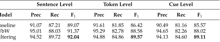
Table 3 shows the performance of the filtering model when using this feature config-uration and testing by 10-fold cross-validation on the training data (BSA and BSP), also contrasting performance with the majority usage baseline. Achieving a sentence-level F1of 92.04 (compared to 89.07 for the baseline), a token-level score of 89.57 (baseline = 86.42), and a cue-level score of 89.11 (baseline = 85.57), it performs significantly better than the baseline. Applying the sign-test as described in Section 3.1, the token-level differences were found to be significant for p < 0.05. It is also clear, however, that the simple baseline appears to be fairly strong.

As discussed previously, part of the motivation for introducing the filtering scheme is to create a model that is as simple as possible without sacrificing performance. In addition to the evaluation scores, therefore, it is also worth noting some statistics related to the classifier and the training data itself. Before looking into the properties of the fil-tering set-up though, let us start, for the sake of comparison, by considering some prop-erties of a learning set-up based on full WbW classification like the model of Velldal, Øvrelid, and Oepen (2010), assuming an identical feature configuration as used for the given filtering model. The row titled WbW in Table 3 lists the development results for this model, and we see that they are slightly lower than for the filtering model (with the differences being significant forα= 0.05). Although precision is slightly higher, recall is substantially lower. Assuming a 10-fold cross-validation scheme like this, the number of training examples presented to the WbW learner in each fold averages roughly 340,000, corresponding to the total number of word tokens. Among these training examples, the ratio of positive to negative examples (cues vs. non-cues) is roughly 1:100. In other words, the data is initially very skewed when it comes to class balance. In terms of the size of the feature set, the average number of distinct feature types per fold, assuming the given feature configuration, would be roughly 2,600,000 under a WbW set-up.

Turning now to the filtering model, the average number of training examples presented to the learner in each fold is reduced from roughly 340,000 to just 10,000. Correspondingly, the average number of distinct feature types is reduced from well above 2,600,000 to roughly 100,000. The class balance among the tokens given to the learner is also much less skewed, with positive examples now averaging 30%, compared to 1% for the WbW set-up. Finally, we observe that the complexity of the model in terms of how many training examples end up as support vectors(SVs) defining the separating hyperplane is also considerably reduced: Although the average number of SVs in each fold corresponds to roughly 14,000 examples for the WbW model, this is down to roughly 5,000 for the final filtered model. Note that for the SVM regularization

Table 3

Development results for detecting speculation CUES: Averaged 10-fold cross-validation results for the cue classifiers on both the abstracts and full papers in the BioScope training data (BSA and BSP).

Sentence Level Token Level Cue Level

Model Prec Rec F1 Prec Rec F1 Prec Rec F1

Baseline 91.07 87.21 89.07 91.61 81.85 86.42 90.49 81.16 85.57

WbW 95.01 88.03 91.37 95.29 82.78 88.58 94.65 82.26 88.02

parameterC, governing the trade-off between training error and margin size, we will always be using the default value set by SVMlight. This value is analytically determined from the training data, and further empirical tuning has in general not led to improve-ments on our data sets.

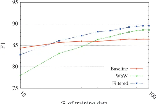
5.2.2 The Effect of Data Size.Given how the filtered classifier treats the set of cues as a closed class, a reasonable concern is its sensitivity to the size of the training set. In order to further assess this effect, we computed learning curves showing how classifier per-formance on the development data changes as we incrementally include more training examples (see Figure 1). For reference we also include learning curves for the word-by-word classifier using the identical feature configuration, as well as the majority usage baseline.

As expected, we see that classifier performance steadily improves as more training data is included. Although additional data would no doubt be beneficial, we reassur-ingly observe that the curve seems to start gradually flattening out somewhat. If we instead look at the performance curve for the WbW classifier we find that, while having roughly the same shape as that of the filtered classifier, although consistently lower, it nonetheless appears to be more sensitive to the size of the training set. Interestingly, we see that the baseline model seems to be the one that is least affected by data size. It actually outperforms the standard WbW model for the first three increments, but at the same time it seems unable to benefit much at all from additional data.

5.2.3 Error Analysis.When looking at the distribution of errors at the cue-level (totaling just below 700 across the 10-fold run), we find that roughly 74% are false negatives. Rather than being caused by legitimate cue words being filtered out during training, however, the FNs mostly pertain to a handful of high-frequency words that are also highly ambiguous. When sorted according to error frequency, the top four candidates alone constitute almost half the total number of FNs:or (24% of the FNs),can(10%),

could(7%), andeither(6%). Looking more closely at the distribution of these words in

Figure 1

Learning curves showing the effect on token-level F1for speculation cues when withdrawing

the training data, it is easy to see how they pose a challenge for the learner. For example, whereas orhas a total of 1,215 occurrences, only 153 of these are annotated as a cue. Distinguishing the different usages from each other can sometimes be difficult even for a human eye, as testified also by the many inconsistencies we observed in the gold-standard annotation of these cases.

Turning our attention to the other end of the tail, we find that just over 40 (8%) of the FNs involve tokens for which there is only asingleoccurrence as a cue in the training data. In other words, these would first appear to be exactly the tokens that we could never get right, given our filtering scheme. We find, however, that most of these cases regard tokens whose one and only appearance as a cue is as part of a multiword cue, although they typically have a high number of othernon-cue occurrences as well. For example, although numberoccurs a total of 320 times, its one and only occurrence as a cue is in the multiword cueaddress a number of questions. Given that this and several other equally rare patterns are not currently covered by our MWC rules in the first place, we would not have been able to get them right even if all the individual tokens had been classified as cues (recall that a true positive at the cue-level requires an exact match of the entire span). In total we find that 16% of the cue-level FNs corresponds to multiword cues.

When looking at the frequency of multiword cues among the false positives, we find that they only make up roughly 5% of the errors. Furthermore, a manual inspection reveals that they can all be argued to be instances of annotation errors, in that we believe these should actually be counted as true positives. Most of them involveindicate thatand

not known, as in the following examples (where the cues assigned by our system are not annotated as cues in BioScope):

(7) In contrast, levels of the transcriptional factor AP-1, which isnot known to be important in B cell Ig production, were reduced by TGF-beta.

(8) Analysis of the nuclear extracts [. . . ]indicated thatthe composition of NF-kappa B was similar in neonatal and adult cells.

All in all, the errors in the FP category make up 26% of the total number of errors. Just as for the FNs, the frequency distribution of the cues involved is quite skewed, with a handful of highly frequent and highly ambiguous cue words accounting for the bulk of the errors: The modalcould (20%), and the adjectives putative(11%), possible

(6%),potential(6%), and unknown(5%). After manually inspecting the full set of FPs, however, we find that at least 60% of them should really be counted as true positives. The following are just a few examples where cues predicted by our classifier are not annotated as such in BioScope and therefore counted as FPs.

(9) IEF-1, a pancreatic beta-cell type-specific complexbelievedto regulate insulin expression, is demonstrated to consist of at least two distinct species, [. . . ]

(10) Wehypothesizethat a mutation of the hGR glucocorticoid-binding domain is the cause [. . . ]

(11) Antioxidants have beenproposedto b e anti-atherosclerotic agents; [. . . ]

One interesting source of real FPs concerns “anti-hedges,” which in the training data appear with a negation and as part of a multiword cue, for exampleno proof. During testing, the classifier will sometimes wrongly predict a word likeproof to be a specu-lation cue, even when it is not negated. Because we already have MWC rules for cases like this (see Section 5.1) it would be easy to also include a check for “negative context,” making sure that such tokens are not classified as cues if the required multiword context is missing.

Before rounding off this section, a brief look at the BioScope inter-annotator agree-ment rates may offer some further perspective on the results discussed here. Note that when creating the BioScope data, the decisions of two independent annotators were merged by a third expert linguist who resolved any differences. The F₁ of each set of annotations toward the final gold-standard cues are reported by Vincze et al. (2008) to be 83.92 / 92.05 for the abstracts and 81.49 / 90.81 for the full papers. (Recall from Table 3 that our cue-level F1for the cross-validation runs on the abstracts and papers is 89.11.) When instead comparing the decisions of the two annotators directly, the F1is reported to be 79.12 for the abstracts and 77.60 for the papers.

5.3 Held-Out Results for Identifying Speculation Cues

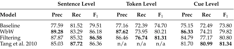
Table 4 presents the final evaluation of the various cue classifiers developed in this section, as applied to the held-out BSE test data. In addition to the evaluation results for our own classifiers, Table 4 also includes the official test results for the system described by Tang et al. (2010). The sequence classifier developed by Tang et al. (2010)—combining a CRF classifier and a large-margin HMM model—obtained the best results for the official Shared Task evaluation for Task 1 (i.e., sentence-level uncertainty detection), as well as the highest cue-level scores.

As seen from Table 4, although the model of Tang et al. (2010) still achieves a slightly higher F₁ (81.34) than our filtered disambiguation model for the cue-level, our model achieves a slightly higher F₁ (86.58) for the sentence-level (yielding the best-published result for this task so far, to the best of our knowledge). The differences are not deemed statistically significant by a two-tailed sign-test, however (p = 0.37). It is interesting to note, however, that the two approaches appear to have somewhat different strengths and weaknesses: Whereas our filtering classifier consistently shows stronger precision (and the WbW model even more so), the model of Tang et al. (2010) is stronger on recall. The sentence-level recall of our filtered classifier is still better than any of the remaining 23 systems submitted for the Shared Task evaluation, however, and, more interestingly, it improves substantially on the recall of the full WbW classifier.

Table 4

Held-out results for identifying speculation cues: Applying the cue classifiers to the 5,003 sentences in BSE— the biomedical papers provided for the CoNLL-2010 Shared Task evaluation.

Sentence Level Token Level Cue Level

Model Prec Rec F1 Prec Rec F1 Prec Rec F1

Baseline 77.59 81.52 79.51 77.16 72.39 74.70 75.15 72.49 73.80

WbW 89.28 83.29 86.18 87.62 73.95 80.21 86.33 74.21 79.82

Filtering 87.87 85.32 86.58 86.46 76.74 81.31 84.79 77.17 80.80

We find that, just as for the development data, the reformulation of the cue clas-sification task as a simple disambiguation problem improves F1 across all evaluation levels, consistently outperforming the WbW classifiers. When computing a two-tailed signed-test for the token-level decisions (where the WbW and filtering model achieves an F1of 80.21 and 81.31, respectively) the differences are not found to be significant (p = 0.12). As discussed in Section 5.2, however, it is important to bear in mind that the size and complexity of the filtered “disambiguation” model is greatly reduced compared to the WbW model, using a much smaller number of features and relevant training examples.

While on the topic of model complexity, it is also worth noting that many of the systems participating in the CoNLL-2010 Shared Task challenge used fairly complex and resource-heavy feature types, being sensitive to properties of document structure, grammatical relations, deep syntactic structure, and so forth (Farkas et al. 2010). The fact that comparable or better results can be obtained using a relatively simplistic approach as developed in this section, with surface-oriented features that are only sensitive to the immediate lexical context, is an interesting result in its own right. In fact, even the simple majority usage baseline classifier proves to be surprisingly competitive: Comparing its sentence-level F1to those of the official Shared Task evaluation, it actually outranks 7 of the 24 submitted systems.

A final point that deserves some discussion is the drop in F1that we observe when going from the development results to the held-out results. There are several reasons for this drop. Section 2.3 discussed how certain overfitting effects might be expected from the GENIA-based pre-processing. In addition to this, it is likely that there are MWC patterns in the held-out data that were not observed in the training data, and that are therefore not covered by our MWC rules. Another factor that may have slightly inflated the development results is the fact that we used a sentence-level rather than a document-level partitioning of the data for cross-validation.

6. Resolving the Scope of Speculation Cues

Once the speculation cue has been determined using the cue detection system described here, we go on to determine the scope of the speculation within the sentence. This task corresponds to Task 2 of the CoNLL-2010 Shared Task. Example (13), which will be used as a running example throughout this section, shows a scope-resolved BioScope sentence where speculation is signaled by the modal verbmay.

(13) {The unknown amino acidmaybe used by these species}.

6.1 A Rule-Based Approach Using Dependency Structures

Øvrelid, Velldal, and Oepen (2010) applied a small set of heuristic rules oper-ating over syntactic dependency structures to define the scope for each cue. In the following we will provide a detailed description of these rules and the syntactic gen-eralizations they provide for the scope of speculation (Section 6.1.2). We will evalu-ate their performance using both gold-standard cues and cues predicted by our cue classifier (Section 6.1.3), in addition to providing an in-depth manual error analysis (Section 6.1.5). We start out, however, by presenting some specifics about the processing of the data; introducing the stacked dependency parser that produces the input to our rules (Section 6.1.1) and quantifying the effect of using a domain-adapted PoS tagger (Section 6.1.4).

6.1.1 Stacked Dependency Parsing.For syntactic analysis we use the open-source Malt-Parser (Nivre, Hall, and Nilsson 2006), a platform for data-driven dependency parsing. For improved accuracy and portability across domains and genres, we make our parser incorporate the predictions of a large-scale, general-purpose Lexical-Functional Gram-mar parser. A technique dubbedparser stackingenables the data-driven parser to learn from the output of another parser, in addition to gold-standard treebank annotations (Martins et al. 2008; Nivre and McDonald 2008). This technique has been shown to provide significant improvements in accuracy for both English and German (Øvrelid, Kuhn, and Spreyer 2009), and a similar set-up using an HPSG grammar has been shown to increase domain independence in data-driven dependency parsing (Zhang and Wang 2009). The stacked parser used here is identical to the parser described in Øvrelid, Kuhn, and Spreyer (2009), except for the preprocessing in terms of tokenization and PoS tagging, which is performed as detailed in Sections 2.1–2.2. The parser combines two quite different approaches—data-driven dependency parsing and “deep” parsing with a hand-crafted grammar—and thus provides us with a broad range of different types of linguistic information to draw upon for the speculation resolution task.

MaltParser is based on a deterministic parsing strategy in combination with treebank-induced classifiers for predicting parse transitions. It supports a rich feature representation of the parse history in order to guide parsing and may easily be extended to take into account additional features. The procedure to enable the data-driven parser to learn from the grammar-driven parser is quite simple. We parse a treebank with the XLE platform (Crouch et al. 2008) and the English grammar developed within the ParGram project (Butt et al. 2002). We then convert the LFG output to dependency structures, so that we have two parallel versions of the treebank—one gold-standard and one with LFG annotation. We extend the gold-standard treebank with additional information from the corresponding LFG analysis and train MaltParser on the enhanced data set. For a description of the parse model features and the dependency substructures proposed by XLE for each word token, see Nivre and McDonald (2008). For further background on the conversion and training procedures, see Øvrelid, Kuhn, and Spreyer (2009).

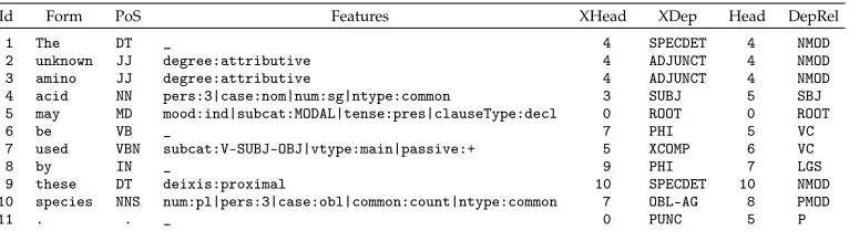
Table 5

Stacked dependency representation of the sentence in Example (13), lemmatized and annotated with GENIA PoS tags, Malt parses (Head, DepRel), and XLE parses (XHead, XDep), as well as other morphological and lexical semantic features extracted from the XLE analysis (Features).

Id Form PoS Features XHead XDep Head DepRel

1 The DT _ 4 SPECDET 4 NMOD

2 unknown JJ degree:attributive 4 ADJUNCT 4 NMOD 3 amino JJ degree:attributive 4 ADJUNCT 4 NMOD 4 acid NN pers:3|case:nom|num:sg|ntype:common 3 SUBJ 5 SBJ 5 may MD mood:ind|subcat:MODAL|tense:pres|clauseType:decl 0 ROOT 0 ROOT

6 be VB _ 7 PHI 5 VC

7 used VBN subcat:V-SUBJ-OBJ|vtype:main|passive:+ 5 XCOMP 6 VC

8 by IN _ 9 PHI 7 LGS

9 these DT deixis:proximal 10 SPECDET 10 NMOD

10 species NNS num:pl|pers:3|case:obl|common:count|ntype:common 7 OBL-AG 8 PMOD

11 . . _ 0 PUNC 5 P

to dependency format (Johansson and Nugues 2007) and extended with XLE features, as described previously. Parsing uses the arc-eager mode of MaltParser and an SVM with a polynomial kernel. When tested using 10-fold cross validation on the enhanced PTB, the parser achieves a labeled accuracy score of 89.8, which is lower than the current state-of-the-art for transition-based dependency parsers (to wit, the 91.8 score of Zhang and Nivre 2011, although not directly comparable given that they test exclusively on WSJ Section 23), but with the advantage of providing us with the deep linguistic information from the XLE.

6.1.2 Rule Overview.Our scope resolution rules take as input a parsed sentence that has been further tagged with speculation cues. We assume thedefault scopeto start at the cue word and span to the end of the sentence (modulo punctuation), and this scope also provides the baseline when evaluating our rules.

In developing the rules, we made use of the information provided by the guidelines for scope annotation in the BioScope corpus (Vincze et al. 2008), combined with manual inspection of the training data in order to further generalize over the phenomena discussed by Vincze et al. (2008) and work out interactions of constructions for various types of cues. In the following, we discuss broad classes of rules, organized by categories of speculation cues. An overview is also provided in Table 6, detailing the source of the syntactic information used by the rule; MaltParser (M) or XLE (X). Note that, as there is no explicit representation of phrase or clause boundaries in our dependency universe, we assume a set of functions over dependency graphs, for example, finding the left- or rightmost (direct)dependentof a given node, or recursively selecting left- or rightmost

descendants.

Coordination. The dependency analysis of coordination provided by our parser makes the first conjunct the head of the coordination. For cues that are coordinating conjunc-tions (PoS tag CC), such as or, we define the scope as spanning the whole coordinate structure, that is, start scope is set to the leftmost dependent of the head of the coordina-tion, and end scope is set to its rightmost dependent (conjunct). This analysis provides us with coordinations at various syntactic levels, such as NP and N, AP and AdvP, or VP as in Example (14):

Table 6

Overview of dependency-based scope rules with information source (MaltParser or XLE), organized by the triggering PoS of the cue.

PoS Description Source

cc Coordinations scope over their conjuncts M

in Prepositions scope over their argument with its descendants M

jj

attr Attributive adjectives scope over their nominal head and its descendants M

jj

pred Predicative adjectives scope over referential subjects and clausal arguments, M, X if present

md Modals inherit subject-scope from their lexical verb and scope over their M, X

descendants

rb Adverbs scope over their heads with its descendants M

vb

pass Passive verbs scope over referential subjects and the verbal descendants M, X

vb

rais Raising verbs scope over referential subjects and the verbal descendants M, X * For multiword cues, the head determines scope for all elements

* Back off from final punctuation and parentheses

Adjectives.We distinguish between adjectives (JJ) inattributive(nmod) function and

adjec-tives inpredicative(prd) function. Attributive adjectives take scope over their (nominal)

head, with all its dependents, as in Example (15):

(15) The{possibleselenocysteine residues}are shown in red, [...]

For adjectives in a predicative function the scope includes the subject argument of the head verb(the copula), as well as a (possible) clausal argument, as in Example (16). The scope does not, however, include expletive subjects, as in Example (17).

(16) Therefore,{the unknown amino acid, if it is encoded by a stop codon, is

unlikelyto exist in the current databases of microbial genomes}. (17) [...] it is quite{likelythat there exists an extremely long sequence that is

entirely unique to U}.

Verbs.The scope of verbal cues is a bit more complex and depends on several factors. In our rules, we distinguishpassiveusages from active usages,raisingverbs from non-raising verbs, and the presence or absence of a subject-control embedding context. The scopes of both passive and raising verbs include the subject argument of their head verb, as in Example (18), unless it is an expletive pronoun, as in Example (19).

(18) {Genomes of plants and vertebratesseemto be free of any recognizable Transibtransposons}(Figure 1).

(19) It has been{suggestedthat unstructured regions of proteins are often involved in binding interactions, particularly in the case of transient interactions}77.

In general, the end scope of verbs should extend over the minimal clause that contains the verbin question. In terms of dependency structures, we define the clause boundary as comprising the chain of descendants of a verb which is not intervened by a token with a higher attachment in the graph than the verbin question.

Prepositions and Adverbs. Cues that are tagged as prepositions (including some com-plementizers) take scope over their argument, with all its descendants, Example (20). Adverbs take scope over their head with all its (non-subject) syntactic descendants Example (21).

(20) {Whetherthe codon aligned to the inframe stop codon is a nonsense codon or not}was neglected [...]

(21) These effects are{probablymediated through the 1,25(OH)2D3 receptor}.

Multiword Cues.In the case of multiword cues, such asindicate thatoreither. . . or, we set the scope of the unit as a whole to the maximal scope encompassing the scopes of both units.

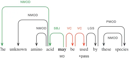
As an illustration of processing by the rules, consider our running Example (13), with its syntactic analysis as shown in Table 5 and the dependency graph depicted in Figure 2. This example invokes a variety of syntactic properties, including parts of speech, argumenthood, voice, and so on. Initially, the scope of the speculation cue is set to default scope. Then the subject control rule is applied, it checks the properties of the verbal argument used, going through a chain of verbal dependents (VC) from the modal verb may (indicated in red in Figure 2). Because it is marked as passive in the LFG analysis (+pass), the start scope is set to include the subject of the cue word (the leftmost descendant [NMOD] of itsSBJdependent, indicated in green in Figure 2).

6.1.3 Evaluating the Rules.Table 7 summarizes scope resolution performance (viewed as a subtask in isolation) against both the CoNLL-2010 shared task training data (BSA and BSP) and held-out evaluation data (BSE), usinggold-standard cues. First of all, we note that the default scope baseline, that is, unconditionally extending the scope of a cue to the end of the sentence, yields much better results for the abstracts than the full papers. The main reason is simply that the abstracts contain almost no cases of sentence final bracketed expressions (e.g., citations and in-text references). Our scope rules improve on the baseline by only 3.8 percentage points on the BSA data (F₁ up from 69.84 to

Figure 2

Table 7

Resolving the scope of gold-standard speculation cues in the development and held-out data using the dependency rules. ForDefault, the scope for each cue is always taken to span rightwards to the end of the sentence.

Data Configuration F1

BSA

Default 69.84

Dependency Rules 73.67

BSP

Default 45.21

Dependency Rules 72.31

BSE

Default 46.95

Dependency Rules 66.60

73.67). For BSP, however, we find that the rules improve on the baseline by as much as 27 points (up from 45.21 to 72.31). Similarly for the papers in the held-out BSE data, the rules improve the F1by 19.7 points (F1up from 46.95 to 66.60).

Comparing to the result on the training data, we observe a substantial drop in performance on the held-out data. There are several possible explanations for this effect. First of all, there may well be some degree of overfitting of our rules to the training data. The held-out data may contain speculation constructions that are not covered by our current set of scope rules, or annotation of parallel constructions may in some cases differ in subtle ways (see Section 6.1.5). The overfitting effects caused by the data dependencies introduced by the various GENIA-based domain adaptation steps, as described in Section 2.3, must also be taken into account.

6.1.4 PoS Tagging and Domain Variation.As mentioned in Section 6.1.1, an advantage of stacking with a general-purpose LFG parser is that it can be expected to aid domain portability. Nonetheless, substantial differences in domain and genre are bound to negatively affect syntactic analysis (Gildea 2001), and our parser is trained on financial news. MaltParser presupposes that inputs have been PoS tagged, however, leaving room for variation in preprocessing. In this article we have aimed, on the one hand, to make parser inputs conform as much as possible to the conventions established in its PTB training data, while on the other hand taking advantage of specialized resources for the biomedical domain.

To assess the impact of improved, domain-adapted inputs on our scope resolution rules, we contrast two configurations: Running the parser in the exact same manner as Øvrelid, Kuhn, and Spreyer (2009)—the first configuration uses TreeTagger (Schmid 1994) and its standard model for English (trained on the PTB) for preprocessing. In the second configuration the parser input is provided by the refined GENIA-based preprocessing described in Section 2.2. Evaluating the two modes of preprocessing on the BSP subset of BioScope using gold-standard speculation cues, our scope resolution rules achieve an F1of 66.31 when using TreeTagger parser inputs, and 72.31 (see Table 7) using our GENIA-based tagging and tokenization combination. These results underline the importance of domain adaptation for accurate syntactic analysis.

thescope-levelF1of the two annotators toward the gold standard to be 66.72 / 89.67 for BSP. Comparing the decisions of the two annotators directly (i.e., treating one of the annotations as gold-standard) yields an F1of 62.50.

Using gold-standard cues, our scope resolution rules fail to exactly replicate the target annotation in 185 (of 668) cases in the papers portion of the training material (BSP), corresponding to an F1 of 72.31 as seen in Table 7. Two of the authors, who are both trained linguists, performed a manual error analysis of these 185 cases. They classify 156 (84 %) as genuine system errors, 22 (12 %) as likely3 annotation errors, and the remaining 7 cases as involving controversial or seemingly arbitrary decisions (Øvrelid, Velldal, and Oepen 2010). Out of the 156 system errors, 85 (55%) were deemed as resulting from missing or defective rules, and 71 system errors (45%) resulted from parse errors. The latter were annotated as parse errors even in cases where there was also a rule error.

The two most frequent classes of system errors pertain to (a) the recognition of phrase and clause boundaries and (b) not dealing successfully with relatively superficial properties of the text. Examples (22) and (23) illustrate the first class of errors, where in addition to the gold-standard annotation we use vertical bars (‘|’) to indicate scope predictions of our system.

(22) [. . . ]{the reverse complement|mR of m will beconsideredto . . . ]|}

(23) This|{mightaffect the results}if there is a systematic bias on the composition of a protein interaction set|.

In our syntax-driven approach to scope resolution, system errors will almost always correspond to a failure in determining constituent boundaries, in a very general sense. In Example (22), for instance, the parser has failed to correctly locate the head of the subject. Example (23), however, is specifically indicative of a key challenge in this task, where adverbials of condition, reason, or contrast frequently attach within the depen-dency domain of a speculation cue, yet are rarely included in the scope annotation. For these system errors, the syntactic analysis may well be correct, although additional information is required to resolve the scope.

Example (24) demonstrates our second frequent class of system errors. One in six items in the BSP training data contains a sentence-final parenthesized element or trailing number (e.g., Examples [18] or [19]); most of these are bibliographic or other in-text references, which are never included in scope annotation. Hence, our system includes a rule to ‘back out’ from trailing parentheticals; in cases such as Example (24), however, syntax does not make explicit the contrast between an in-text reference versus another type of parenthetical.

(24) More specifically,{|the bristle and leg phenotypes arelikelyto result from reduced signaling by Dl|(and not by Ser)}.

Moving on to apparent annotation errors, the rules for inclusion (or not) of the subject in the scope of verbal speculation cues and decisions on boundaries (or internal structure) of nominals seem problematic—as illustrated in Examples (25) and (26).4

(25) [. . . ] and|this is also{thoughtto be true for the full protein interaction networks we are modeling}|.

(26) [. . . ]|redefinition of{one of them isfeasible}|.

Finally, the difficult corner cases invoke non-constituent coordination, ellipsis, or NP-initial focus adverbs—and of course interactions of the phenomena discussed herein. Without making the syntactic structures assumed explicit, it is often very diffi-cult to judge such items.

6.2 A Data-Driven Approach Using an SVM Constituent Ranker

The error analysis indicated that it is often difficult to use dependency paths to define phenomena that actually correspond to syntactic constituents. Furthermore, we felt that the factors governing scope resolution would be better expressed in terms of soft con-straints instead of absolute rules, thus enabling the scope resolver to consider a range of relevant (potentially competing) contextual properties. In this section we describe experiments with a novel approach to determining the in-sentence scope of speculation that, rather than using manually defined heuristics operating on dependency structures, instead uses adata-drivenapproach, ranking candidate scopes on the basis ofconstituent trees. More precisely, our parse trees are licensed by the LinGOEnglish Resource Gram-mar(ERG; Flickinger [2002]), a general-purpose, wide-coverage grammar couched in the framework of an HPSG (Pollard and Sag 1987, 1994). The approach rests on two main assumptions: Firstly, that the annotated scope of a speculation cue corresponds to a syntactic constituent and secondly, that we can automatically learn a ranking function that selects the correct constituent.

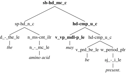
Our ranking approach to scope resolution is abstractly related to statisticalparse selection, and in particular work on discriminative parse selection for unification based grammars, such as those by Johnson et al. (1999), Riezler et al. (2002), Malouf and van Noord (2004), and Toutanova et al. (2005). The overall goal is to learn a function for ranking syntactic structures, based on training data that annotates which tree(s) are correct and incorrect for each sentence. In our case, however, rather than discriminating between complete analyses for a given sentence, we want to learn a ranking function over candidatesubtrees(i.e., constituents) within a parse (or possibly even within several parses). Figure 3 presents an example derivation tree that represents a complete HPSG analysis. Starting from the cue and working through the tree bottom–up, there are three candidate constituents to determine scope (marked in bold), each projecting onto a substring of the full utterance, and each including at least the cue. Note that in the case of multiword cues the intersection of each word’s candidates is selected, ensuring that all cues appear within the scope projected by the candidate constituents.

The training data is then defined as follows. Given a parsed BioScope sentence, the subtree that corresponds to the annotated scope for a given speculation cue will

Figure 3

An example derivation tree. Internal nodes are labeled with ERG rule identifiers; common HPSG constructions near the top (e.g., subject-head, head-complement, adjunct-head), and lexical rules (e.g., passivization of verbs or plural formation of nouns) closer to the leaves. The preterminals are so-called LE types, corresponding to fine-grained parts of speech and reflecting close to a thousand lexical distinctions.

be labeled as correct. Any other remaining constituents that also span the cue are labeled as incorrect. We then attempt to learn a linear SVM-based scoring function that reflects these preferences, using the implementation of ordinal ranking in the SVMlight toolkit (Joachims 2002). Our definition of the training data, however, glosses over two important details.

Firstly, the grammar will usually license not just one, but thousands or even hun-dreds of thousands of different parses for a given sentence which are ranked by an underlying parse selection model. Some parses may not necessarily contain a subtree that aligns with the annotated scope. We therefore experiment with defining the training data relative ton-best lists of available parses. Secondly, the rate of alignment between annotated scopes and constituents of parsing results indicates the upbound per-formance: For inputs where no constituents align with the correct scope substring, a correct prediction will not be possible. Searching the n-best parses for alignments enables additional instances of scope to be presented to the learner, however.

In the following, Section 6.2.1 summarizes the general parsing setup for the ERG, as well as our rationale for the use of HPSG. Section 6.2.2 provides an empirical assessment of the degree to which ERG analyses can be aligned with speculation scopes in BioScope and reviews some frequent sources of alignment failures. After describing our feature types for representing candidate constituents in Section 6.2.3, Section 6.2.4 details the tuning of feature configurations and other ranker parameters. Finally, Section 6.2.5 provides an empirical assessment of stand-alone ranker performance, before we discuss the integration of the dependency rules with the ranking approach in Section 6.3.

representation—HPSG derivation trees, as depicted in Figure 3—where all contextual information that we expect to be relevant for scope resolution is readily accessible.

For parsing biomedical text using the ERG, we build on the same preprocessing pipeline as described in Section 2. A lattice of tokens annotated with parts of speech and named entity hypotheses contributed by the GENIA tagger is input to the PET HPSG parser (Callmeier 2002), a unification-based chart parser that first constructs a packed forest of candidate analyses and then applies a discriminative parse ranking model to selectively enumerate ann-best list of top-ranked candidates (Zhang, Oepen, and Carroll 2007). To improve parse selection for this kind of data, we re-trained the discriminative model following the approach of MacKinlay et al. (2011), combining gold-standard out-of-domain data from existing ERG treebanks with a fully automated procedure seeking to take advantage of syntactic annotations in the GENIA Treebank. Although we have yet to pursue domain adaptation in earnest and have not systemat-ically optimized the parse selection component for biomedical text, model re-training contributed about a one-point F1improvement in stand-alone ranker performance over the parsed subset of BSP (compare to Table 8).

As the ERG has not previously been adapted to the biomedical domain, unknown word handling in the parser plays an important role. Here we build on a set of somewhat underspecified “generic” lexical entries for common open-class categories provided by the ERG (thus complementing the 35,000-entry lexicon that comes with the grammar), which are activated on the basis of PoS and NE annotation from preprocess-ing. Other than these, there are no robustness measures in the parser, such that syntactic analysis will fail in a number of cases, to wit, when the ERG is unable to derive a complete, well-formed syntactic structure for the full input string. In this configuration, the parser returns at least one derivation for 91.2% of all utterances in BSA, and 85.6% and 81.4% for BSP and BSE, respectively.

6.2.2 Alignment of Constituents and Scopes.The constituent ranking approach makes ex-plicit an assumption that is also present at the core of our dependency-based heuristics (viz., the expectation that scope boundaries align with the boundaries of syntactically meaningful units). This assumption is motivated by general BioScope annotation prin-ciples, as Vincze et al. (2008) suggest that the “scope of a keyword can be determined on the basis of syntax.” To determine the degree to which ERG analyses conform to this expectation, we computed the ratio of alignment between scopes and constituents (over parsed sentences) in BioScope, considering various sizes of n-best lists of parses. To improve alignment we also apply a small number of slackening heuristics. These rules allow (a) minor adjustments of scope boundaries around punctuation marks

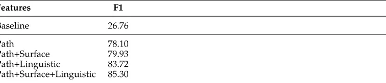
Table 8

Ranker optimization on BSP: Showing ranker performance for various feature type combinations compared with a random-choice baseline, only considering instances where the gold-standard scope aligns to a constituent within the 1-best parse.

Features F1

Baseline 26.76

Path 78.10

Path+Surface 79.93

Path+Linguistic 83.72

(specifically, utterance-final punctuation is never included in BioScope annotations, yet the ERG analyzes most punctuation marks as pseudo-affixes on lexical tokens; see Fig-ure 3). Furthermore, the slackening rules (b) reduce the scope of a constituent to the right when it includes a citation (see the discussion of parentheticals in Section 6.1.5); (c) re-duce the scope to the left when the left-most terminal is an adverband is not the cue; and (d) ensure that the scope starts with the cue when the cue is a noun. Collectively, these rules improve alignment (over parsed sentences) in BSP from 74.10% to 80.54%, when only considering the syntactic analysis ranked most probable by the parse selection model. Figure 4 further depicts the degree of alignment between speculation scopes and constituents in then-best derivations produced by the parser, again after application of the slackening rules. Alignment when inspecting only the top-ranked parse is 84.37% for BSA and 80.54% for BSP. Including the top 50-best derivations improves alignment to 92.21% and 88.93%, respectively. Taken together with an observed parser coverage of 85.6% for BSP, these results mean that for only about 76% of all utterances in BSP can the ranker potentially identify a constituent matching the gold-standard scope.

To shed some light on the cases where wefailto find an alignment, we manually inspected all utterances in the BSP segment for which there were (a) syntactic analyses available from the ERG and (b) no candidate constituents in any of the top-fifty parses that mapped onto the gold-standard scope (after the application of the slackening rules). The most interesting cases from this non-alignment analysis are ones judged as “non-syntactic” (25% of the total mismatches), which we interpret as violating the assumption of the annotation guidelines under any possible interpretation of syntactic structure. Following are select examples in this category:

(27) This allows us to{address a number of questions: what proportion of each organism’s protein interaction network [. . . ] can b e attrib uted to a known domain-domain interaction}?

(28) As{suggestedin 18, by making more such data sets available, it will be possib le to [. . . ] determine the most likely human interactions}.

Figure 4