Localization dynamics in a binary two dimensional cellular automaton: The Diffusion Rule

Photocopying permitted by license only a member of the Old City Publishing Group

Localization Dynamics in a Binary

Two-dimensional Cellular Automaton:

the Diffusion Rule

Genaro J. Martínez1,2, Andrew Adamatzky2 and Harold V. McIntosh3

1_{Departamento de Posgrado, Escuela Superior de Cómputo,}

Instituto Politécnico Nacional, México E-mail: [email protected]

http://uncomp.uwe.ac.uk/genaro/

2_{Faculty of Computing, Engineering and Mathematical Sciences,}

University of the West of England, Bristol, United Kingdom E-mail: [email protected]

http://uncomp.uwe.ac.uk/adamatzky/

3_{Departamento de Aplicación de Microcomputadoras, Instituto de Ciencias,}

Universidad Autónoma de Puebla, Puebla, México E-mail: [email protected] http://delta.cs.cinvestav.mx/∼mcintosh/

Received: August 6, 2006. Accepted: December 2, 2006.

We study a two-dimensional cellular automaton (CA), called Diffusion

Rule (DR), which exhibits diffusion-like dynamics of propagating patterns.

In computational experiments we discover a wide range of mobile and stationary localizations (gliders, oscillators, glider guns, puffer trains, etc), analyze spatio-temporal dynamics of collisions between localizations, and discuss possible applications in unconventional computing.

Keywords: Cellular automata, Diffusion Rule, semi-totalistic rules, particle collisions, mean field theory, reaction-diffusion, unconventional computing.

1 INTRODUCTION

state 1 belongs to another specified interval.

From 1296 cell-state transition rules, we selected a set of rules with complex behavior [4]. Amongst the complex rules, namely inG-class of morphological classification [4], we located so-called Diffusion Rule. CA governed by this rule often exhibits slowly non-uniformly growing patterns, resembling diffu-sive patterns in chemical systems with non-trivial coefficients of diffusion, or reaction-dependent diffusion coefficients, so the name of the rule.

The rule simulates sub-excitable [36] medium-like mode of perturbation propagation—cell in state 0 takes state 1 if there are exactly two neighbors in state 1, otherwise the cell remains in state 0, and, conditional inhibition—cell in state 1 remains in state 1 if there are exactly seven neighbors in state 1, otherwise the cell switches to state 1.

In present paper we are trying to answer the following questions. Is there a reaction-diffusion binary-state CA that express complex dynamic? Can we demonstrate that CA exhibits non-stationary growth of reaction-diffusion pat-terns? Do stationary or mobile generators of localizations, glider guns, exist in binary-state reaction-diffusion CA? Can the reaction-diffusion CA simulate an effective procedure and therefore be universal?

CA with space-time dynamics similar to that in spatially extended chem-ical systems are studied from early days of CA theory and applications [35], however most rules discovered so far lack minimality (some of the rules employ dozens of cell-states). Methods of selecting the rules also widely vary depending on theoretical frameworks, e.g. probabilistic spaces [20, 38] and genetic algorithms [14, 32]. Therefore, we envisage a strong need for a sys-tematic analysis of propagating patterns like those observed in the Diffusion Rule. The propagating patterns are of upmost importance in modern com-puter science because such patterns play a vital role in developing novel and emerging computing paradigms and architectures, particularly collision-based computing [1, 3, 23].

We must mention that various authors have already obtained pioneering results in the studied rule. Magnier et al. discovered three primary gliders [33]. David Eppstein found four gliders known, already incorporated in our frame-work, and four new gliders which were novel for us (Fig. 4 (q) (t) and (u)).1The glider traveling along diagonals of the lattice (Fig. 4 (v)) was firstly recorded by Amling in 2002 (see Eppstein’s web site). Finally, a glider gun and three puffer trains were discovered by Wótowicz.2

Diffusion Rule CA is just one of many complex CA3 exhibiting mobile localizations. Other famous examples include semi-totalistic rules as the Game of Life [10, 17], Brain’s-brain and Critters rules [34], High Life [9], Life 1133 [22], Life Without Death [18], and Life variantB35/S236.4Other variant is with Larger than Life [16] and the Beehive and Spiral rules hexagonal CA [5,6,39], more recent candidates were proposed by George Maydwell with Hexagonal Life and Hexagonal Long Life rules.5Amongst 3D binary state CA supporting gliders Life 4555 and Life 5766 by Carter Bays [7, 8] are most widely known. In 1D there are Rule 110 [13,26,30,37] and Rule 54 [11,21,25] CA, which support an impressive range of mobile localizations.

Our paper is structured as follows. In Sect. 2 we introduce basic concepts of CA model under investigation. Section 3 introduces results of statistical analysis of the Diffusion Rule using mean field theory. In Sect. 4 we present basic structures discovered in the Diffusion Rule CA. Section 5 compiles a catalogs of non-trivial interactions between mobile localizations, which could be used to designing basic elements of collision-based computers. In Sect. 6 we highlight our achievements in analysis of the Diffusion Rule and prospects for future studies.

2 BASIC NOTATIONS

We study family of 2D binary-state cellular automaton (CA) defined by tuple Z2_{, , u, f, whereZis the set of integers, every cellx ∈ Z}2 _{has eight} neighbors, orthogonal and diagonal (i.e. classical Moore’s neighborhood) u(x)= {y∈Z:x=yand|x−y| ≤1}, = {0,1}is the set of states, and f is a local transition function defined as follows:

xt+1=f (u(xt))

=

1, if(xt =0 andσ_xt ∈ [θ1, θ2])or(xt =1 andσ_xt ∈ [δ1, δ2])

0, otherwise

(1)

whereσ_xt = |{y∈u(x):yt =1}|, andθ1, θ2, δ1, δ2are some fixed parameters such that 0≤θ1≤θ2≤8 and 0≤δ1≤δ2≤8.

We can write the rule asR(δ1δ2θ1θ2)or likeBθ1· · ·θ2/Sδ1· · ·δ2more traditional code. Also, the rule can be interpreted as a simple discrete model

3_{http://uncomp.uwe.ac.uk/genaro/otherRules.html} 4_{http://www.ics.uci.edu/∼eppstein/ca/b35s236/}

Game Life, when intervals[δ1, δ2]and[θ1, θ2]are interpreted as intervals of survival and birth, respectively.

In our previous paper [4] we morphologically classified all 1296 rules, and studied how changes in parametersR(δ1δ2θ1θ2)of cell-state transition rule influence space-time dynamics. For example, we discovered [4] a small subset of rules Life 2c22,62≤c≤8, which could be interpreted as quasi-chemical precipitating systems. For parameter set[θ1, θ2] = [22][1, 4], the system is transformed into 2+-medium, CA model of excitable system in sub-excitable mode.

We have found a cluster of semi-totalistic rules supporting structures of the Diffusion Rule. They areB2/S2. . .8 called Lifedc227whered andctake values between 2 and 8, andd≤c. Therefore, we found that the ruleB2/S7 orR(7722)exhibits most reach dynamics of localized patterns amongst all the rules studied by us. Rules of the local transition are simple:

1. A cell in state 0 will take state 1 if it has exactly two neighbors in state 1, otherwise cell remains in state 0.

2. A cell in state 1 remains in state 1 if it has exactly seven neighbors in state 1, otherwise cell takes state 0.

3 MEAN FIELD APPROXIMATION

Mean field theory is a proved technique for discovering statistical properties of CA without analyzing evolution spaces of individual rules [12, 20, 28]. The method assumes that elements of the set of states are independent, uncor-related between each other in the rule’s evolution space. Therefore we can study probabilities of states in neighborhood in terms of probability of a sin-gle state (the state in which the neighborhood evolves), thus probability of a neighborhood is the product of the probabilities of each cell in the neigh-borhood. Using this approach we can construct mean field polynomial for a semi-totalistic evolution rule [24] as follow:

pt+1=

δ2

v=δ1

n−1 v

pv_t+1q_tn−v−1+

θ2

v=θ1

n−1 v

pv_tq_tn−v (2)

wheren represents the number of cells in neighborhood, v indicates how often state 1 occurs in Moore’s neighborhood,n−vshows how often state 0

(a) (b) (c)

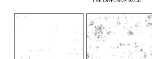
FIGURE 1

Three random initial densities for the Diffusion Rule: (a) 0.004, (b) 0.013 and (c) 0.995 respectively, on lattices of 200×200 to 18 generations.

occurs in the neighborhood,pt is a probability of cell being in state 1,qt is a

probability of cell being in state 0.

On the basis of outcomes of computational experiments we can sug-gest intervals of extreme densities of initial random configurations which leads to the emergence of localizations in the Diffusion Rule. In the lower limit best densitiesd are 0.004< d <0.015 and in the upper limit they are 0.992< d <0.997 for the first 15–20 steps of evolution (Fig. 1). CA start-ing its evolution in random configuration with lower density of 1-states exhibit stationary or mobile self-localizations (like gliders or oscillators) at the beginning of the evolution, however in many cases collisions between mobile localizations leads to catastrophes, when 1-state patterns spread all over the lattice. Random initial configurations with higher (upper limit) den-sity of 1-states produce either vanishing reactions between localizations or symmetrical growing patterns emerged as unions of two or more gliders.

Thus, the mean field polynomial for the Diffusion Rule is following:

pt+1=8p_t8qt+28pt2qt7 (3)

The fixed point is 0.236 that represents configurations with large density of 1-states emerging from any random initial condition (we should note that the fixed point for Conway’s Game of Life is 0.37); this represents global density of 1-states necessary for evolution dynamics to stabilize. Also, we can see an unstable fixed point 0.05 (Fig. 2), that implies the existence of regions with unpredictable behavior or complex dynamic [28].

FIGURE 2

Diagram of mean field polynomial for the Diffusion Rule.

We must also mention that the probability to find ‘interesting’ behavior is very low, about 0.05. Perhaps, this may be the reason why the Diffusion Rule was not studied before – when observing evolution from random configuration one more likely (with probability 0.3) to encounter a catastrophe (e.g. when placing three cells anywhere in Moore’s neighborhood, just not in one line) then stable mobile localization.

4 THE DIFFUSION RULE UNIVERSE

In present section we uncover a range of basic structures, stationary and mobile localizations, generators of localizations and polymer-like structures formed of the mobile localizations.

4.1 Mobile self-localizations

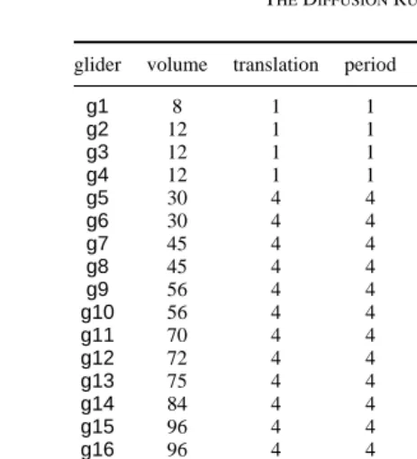
In computational experiments with the Diffusion Rule CA we discovered 26 mobile self-localizations—gliders or particles—traveling orthogonally or diagonally in the lattice. Properties of the gliders, including volume, speed, direction of motion are listed in Table 1.

glider volume translation period speed weight move

g1 8 1 1 c/1 4 orthogonal

g2 12 1 1 c/1 4 orthogonal

g3 12 1 1 c/1 4 orthogonal

g4 12 1 1 c/1 4 orthogonal

g5 30 4 4 c/1 7 orthogonal

g6 30 4 4 c/1 7 orthogonal

g7 45 4 4 c/1 14 orthogonal

g8 45 4 4 c/1 14 orthogonal

g9 56 4 4 c/1 14 orthogonal

g10 56 4 4 c/1 14 orthogonal

g11 70 4 4 c/1 24 orthogonal

g12 72 4 4 c/1 14 orthogonal

g13 75 4 4 c/1 18 orthogonal

g14 84 4 4 c/1 24 orthogonal

g15 96 4 4 c/1 18 orthogonal

g16 96 4 4 c/1 22 orthogonal

g17 96 4 4 c/1 26 orthogonal

g18 96 4 4 c/1 30 orthogonal

g19 112 4 4 c/1 26 orthogonal

g20 126 4 4 c/1 26 orthogonal

g21 144 4 4 c/1 26 orthogonal

g22 144 4 4 c/1 30 orthogonal

g23 210 4 4 c/1 38 orthogonal

g24 338 2 4 c/2 52 orthogonal

g25 405 2 4 c/2 79 orthogonal

g26 576 2 8 c/4 75 diagonal

TABLE 1

Properties of gliders in the Diffusion Rule CA

(a) (b) (c) (d)

FIGURE 3

Configurations of minimal, or primary, gliders in the Diffusion Rule: (a)g1glider, (b)g2glider, (c)g3glider and (d)g4glider.

period. Fifth column shows the speed =c/period, wherecis the maximum speed. Sixth column is the weight that represents the number of cells with state 1 within glider’s volume. The last column indicates whether or not glider moves along columns and rows, or diagonals.

There are two types of gliders—primary and compound [26, 38]: a primary glider can not be decomposed into smaller mobile localizations, a compound glider is made of at least two primary gliders.

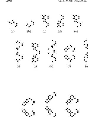
4.2 Oscillators

(a) (b) (c) (d) (e) (f) (g) (h)

(i) (j) (k) (l) (m) (n) (o)

(p) (q) (r) (s) (t)

(u) (v)

FIGURE 4

Twenty two compound gliders in the Diffusion Rule CA: (a)g5, (b)g6, (c)g7, (d)g8, (e)g9, (f)g10, (g)g11, (h)g12, (i)g13, (j)g14, (k)g15, (l)g16, (m)g17, (n)g18, (o)g19, (p)g20, (q)g21, (r)g22, (s)g23, (t)g24, (u)g25and (v)g26gliders, respectively.

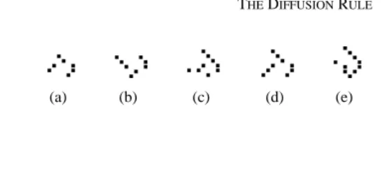
Flip-flop configurations areo1ando2oscillators both structures flipping at 45◦. Blinkers of period four areo3,o4ando5oscillators. Table 2 shows basic characteristics of each oscillator.

(a) (b) (c) (d) (e)

FIGURE 5

Five oscillators in the Diffusion Rule CA: (a)o1and (b)o2are flip-flops, (c)o3, (d)o4and (e)o5are blinkers, respectively.

oscillator volume period weight

o1 4 2 2

o2 9 2 3

o3 10 4 4

o4 16 4 4

o5 30 4 8

TABLE 2

Properties of oscillators in the Diffusion Rule CA

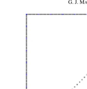
4.3 Avalanches

Avalanches are novel structures, have not described before in related stud-ies. They are assembles of adjacent gliders that cause explosive growth of rhomboid shaped patterns with deterministic edges and quasi-chaotic interior. Avalanches can be constructed from various compositions of adjacent gliders. Figure 6 shows an avalanche produced in composition of two g1 glid-ers, adjacent at 90◦; this avalanche pattern grows diagonally inside the third quadrant. The minimal volume of an avalanche is 4×4 with eight cells in state 1.

(a) (b) (c)

FIGURE 6

(a) (b)

FIGURE 7

Construction of the symmetrical avalanches: (a) symmetrical growth initiated by twog4gliders, configuration at 237th step of evolution, (b) avalanche pattern with non-trivial internal symmetries produced by assembly of twog2glider and twog3gliders, configuration at 237th step of evolution.

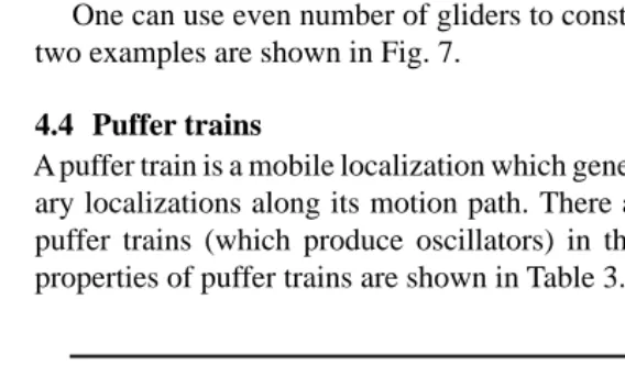
One can use even number of gliders to construct symmetrical avalanches, two examples are shown in Fig. 7.

4.4 Puffer trains

A puffer train is a mobile localization which generate (leaves traces) of station-ary localizations along its motion path. There are 16 known types of stable puffer trains (which produce oscillators) in the Diffusion Rule CA. Basic properties of puffer trains are shown in Table 3.

puffer train produce volume translation period speed weight move

p1 o3 30 4 4 c/1 7 orthogonal

p2 o1 35 4 4 c/1 8 orthogonal

p3 o1 42 4 4 c/1 9 orthogonal

p4 o1 42 4 4 c/1 9 orthogonal

p5 o1 42 4 4 c/1 10 orthogonal

p6 o1 54 4 4 c/1 13 orthogonal

p7 o1 56 4 4 c/1 9 orthogonal

p8 2×o1 63 4 4 c/1 14 orthogonal

p9 o1 63 4 4 c/1 15 orthogonal

p10 2n×o1 65 4 4 c/1 14 orthogonal

p11 2×o1 80 4 4 c/1 17 orthogonal

p12 o1 84 4 4 c/1 11 orthogonal

p13 2×o1 90 4 4 c/1 11 orthogonal

p14 2×o1 105 4 4 c/1 15 orthogonal

p15 2n×o1 120 4 4 c/1 28 orthogonal

p16 o1∨ 242 4 4 c/1 22 orthogonal

TABLE 3

(a) (b) (c) (d) (e) (f) (g) (h)

(i) (j) (k) (l) (m) (n) (o)

FIGURE 8

Fifteen puffer trains observed in evolution of the Diffusion Rule CA: (a)p1, (b)p2, (c)p3, (d)p4, (e)p5, (f)p6, (g)p7, (h)p8, (i)p9, (j)p10, (k)p11, (l)p12, (m)p13, (n)p14and (o)p15

puffer trains, respectively.

(a) (b) (c)

(d) (e) (f)

FIGURE 9

Specialp16puffer train similar to spaceships.

A particular case of puffer train is shown in Fig. 9. This puffer bears frag-ments ofg4glider. All configurations of the puffer are displayed in Fig. 9, and there we can see that configurations shown in Fig. 9(c) (d) (e) and (f) can be interpreted as spaceships.

Moreover, the Diffusion Rule CA exhibits dozens of non-stable puffer trains. In the Fig. 10 we see five non-stable puffer trains, which produce asymmetrically growing, or quasi-chaotic, patterns. All discovered non-stable puffer trains have speed 1/cand period four.

4.5 Mobile glider guns

(a) (b) (c) (d) (e)

FIGURE 10

Some non-stable puffer trains.

gun produce volume translation period speed weight move

gun1 g1 30 4 4 c/1 7 orthogonal

gun2 g4 50 4 4 c/1 9 orthogonal

gun3 g4 50 4 4 c/1 9 orthogonal

gun4 g4 60 4 4 c/1 9 orthogonal

gun5 g4 60 4 4 c/1 9 orthogonal

gun6 g4 72 4 4 c/1 15 orthogonal

gun7 g2∧g3 72 4 4 c/1 16 orthogonal

gun8 2×g4 80 4 4 c/1 14 orthogonal

gun9 2×g4 90 4 4 c/1 14 orthogonal

gun10 g1∧g4 143 4 4 c/1 15 orthogonal

gun11 2×g1 154 4 4 c/1 24 orthogonal

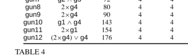
gun12 (2×g4)∨g4 176 4 4 c/1 19 orthogonal

TABLE 4

Characteristics of glider guns in the Diffusion Rule CA. Second column of the table shows what type of glider each glider gun produces

(a) (b) (c) (d) (e) (f) (g) (h) (i) (j) (k)

FIGURE 11

Configurations of glider guns in the Diffusion Rule CA.

Basic parameters of the twelve glider guns are shown in Table 4 and gun’s configurations in Fig. 11. The most remarkable feature is that all primary gliders can be produced by glider guns. Some glider guns can generate two types of gliders at once, thusgun7(Fig. 11f) generatesg2andg3gliders at the same time, however both gliders travel coupled in pairs.

(a) (b) (c)

FIGURE 12

Extendable glider gun in the Diffusion Rule CA.

So far we did not find glider guns which produce diagonally-moving streams of gliders, neither guns generating compound gliders or station-ary guns.

4.6 Glider gun and puffer train

There is at least one special mobile structure that combines in itself properties of both glider gun and puffer train. Figure 13 shows glider gun producingg1 glider ando1oscillator each 4th step of CA evolution. This puffer-gun moves orthogonally, has a volume of 70 cells and weights 12 units.

4.7 Avalanche gun

Avalanche gun is another remarkable example of mobile generators (Fig. 14). The mobile gun produces an avalanche every 4th step of CA evolution.

However, life-time of the gun producing each avalanche is short: when avalanche produced by the gun it grows and then destroys the next avalanche produced.

t=0 t=1 t=2 t=3 t=4

FIGURE 13

Configurations of puffer-gun in the Diffusion Rule CA.

t=0 t=1 t=2 t=3 t=4

(a)

t=40

(b)

FIGURE 14

mously rich dynamics of collisions between mobile and stationary objects. This section studies the outcomes of the collision reactions.

5.1 Forming diffusing patterns by collisions

Gliders colliding in the Diffusion Rule CA can produce an explosively growing diffusion-like pattern, the diffusive patterns do usually have non-stationary boundaries and they exhibit quasi-chaotic internal dynamics.

Two most distinct examples are shown in Fig. 15. In first example (Fig. 15(a)),g4glider collides withg3andg2gliders, diffusion pattern pro-duced is ‘lead’by three gliders and puffer train. In second example (Fig. 15(b)), twog4gliders collides with twog1gliders. The reaction produces multiple gliders, puffer trains, oscillators, and even vertical glider guns during their collision dynamics.

5.2 Reactions between propagating patterns 5.2.1 Soliton-like reaction

In certain initial conditions gliders collide similarly to solitons, namely they restore their structure and velocity vector after collisions. In Fig. 16 we can see snapshots of the head-on collision dynamics between twog4gliders (begin at even distance before collision). When the gliders collide they temporarily lose their stability, produce varieties of transient structures. After few steps of evolution the gliders are restored and transient structures are annihilated.

(a) (b)

FIGURE 15

Examples of diffusion-like patterns produced in collision between gliders in the Diffusion Rule CA. (a) pattern produced at 260th step of evolution after collision betweeng4,g2gliders and

t=0 t=1 t=2 t=3 t=4 t=5 t=6 t=7

t=8 t=9 t=10 t=11 t=12

t=13 t=14 t=15 t=16

FIGURE 16

Soliton-like reaction between twog4gliders.

At the moment, there is only a reaction soliton-like perhaps some others examples exist with more bigger gliders but initially have not more examples.

5.2.2 Eater reaction

Eaters are stationary localizations which destroy gliders colliding into them. The most simple eater is built witho1oscillator. This eater destroysg1gliders but is shifted four cells along the glider’s initial direction of motion. Both g1and g2gliders are destroyed when they collide with the eater built of o3oscillator. In Fig. 17(a) you can see an eater made of twoo3oscillators destroyingg1andg4gliders. A ‘universal’ eater, which destroys all types of primary gliders is illustrated in Fig. 17(b).

Using eaters one can control glider streams emitted by glider guns, thus in Fig. 18 we can see how the eater eliminatesg1gliders produced bygun1. There is at least one mobile eater of gliders, this is g24 glider that eats g1gliders.

5.2.3 Delay reaction

The basic delay reaction can be implemented wheng3glider collides with g4glider and changed tog4glider in the result of collision, and the original

(a) (b)

FIGURE 17

Examples of eater configurations in the Diffusion Rule CA.

t=0 t=1 t=2 t=3 t=4 t=5 t=6

FIGURE 18

FIGURE 19

Delay reaction in the Diffusion Rule CA: (a) initial position of gliders before collision, (b) final result of delay operation, the glider traveling west delayed and translated southward.

g4glider delayed for two time steps but also translated southward one cell per collision (Fig. 19).

5.2.4 Multiplication and reduction reactions

A typical reaction of glider multiplication is shown in Fig. 20(a): twog4gliders are involved in head-on collision, with odd distance between glider heads before collision, four newg4gliders are produced in result of the collision. Reduction is implemented as multiplication of gliders, where gliders in the multiplied columns are in proximity of each other. As shown in Fig. 20(b), when we collide two rows ofg4gliders, four gliders in each row (eight gliders in total are involved in the collision), then just four new gliders are produced. Adjusting distance between gliders in colliding columns of gliders we can achieve almost any (but odd) result of multiplication (Fig. 20(c)).

Using multiplication reactions we can also construct arbitrary packages of gliders. For example, to construct a stream of packages, six gliders per package, we collide stream of four-glider g4packages traveling west with a pair ofg4gliders traveling east (Fig 21(a)). Sequentially, all four-glider packages are transformed to six-glider packages (Fig. 21(b)), the operation is halted by pairg3gliders.

5.2.5 Reflection reaction

We discovered nine types of reflection-type collisions between stationary and mobile self-localizations. Let us discuss some examples shown in Fig. 22. When twog1gliders collide with each other (head-on collision, even distance, with slight shift between gliders along south-north axis) twog4gliders are

t=0 t=8

(a)

t=0 t=8

(b)

t=0 t=8

(c)

FIGURE 20

(a)

(b)

FIGURE 21

Constructing packages ofg4gliders by multiplication reaction. (a) initial configuration, (b) final configuration, recorded after 186th steps of evolution.

t=0 t=7

(a)

t=0 t=6

(b)

t=0 t=6

(c)

t=0 t=6

(d)

t=0 t=5

(e)

t=0 t=9

(f)

FIGURE 22

Collisions leading to reflections: (a) twog1gliders collide with each other, (b)g4glider collides witho1oscillator, (c)g2glider collides witho1oscillator, (d)g3glider collides witho1oscillator, (e)g1glider collides witho5oscillator, (f)g3glider collides witho3oscillator.

generated; theseg4gliders move in the direction perpendicular to original trajectories of colliding gliders (Fig. 22(a)). Glider colliding witho1oscillator is reflected at the angle 90◦, as shown for collision ofg2,g4andg3gliders witho1oscillator (Fig. 22(b) (c) (d)).

Gliders can also be derived in addition of reflections, when colliding with stationary localizations. Thus, when ag1glider collides with ao5oscillator, twog1gliders (going in opposite directions to each other) are generated and follow trajectories perpendicular to original trajectory of collidedg1gliders (Fig. 22(e)).8Similarly, wheng3glider collides witho3oscillator, twog4 gliders are produced (Fig. 22(f)).

5.2.6 Annihilation reaction

Significant amount of collisions between localizations in the Diffusion Rule CA leads to annihilation of colliding patterns. Few examples of initial

(a) (b) (c) (d) (e) (f)

(g) (h) (i) (j) (k)

FIGURE 23

Initial positions of colliding gliders and oscillators leading to annihilation reaction. (a)–(f) binary collisions, (g)–(k) multiple collisions.

configurations of colliding objects (leading to annihilation) are shown in Fig. 23, for binary collisions between gliders (Fig. 23(a)–(f)) and multiple collisions between gliders and oscillators (Fig. 23(g)–(k)).

5.3 Computation in the Diffusion Rule

Basic operations necessary to implement a functionally complete set of logical gates can be derived from collision dynamics presented in Fig. 22. Follow-ing paradigms of collision-based computFollow-ing [2] we encode logicalTruthby presence of a glider or an oscillator, while absence of mobile or stationary objects corresponds to logicalFalsity.

Namely, Fig. 22(b) (c) (d) demonstrate that stationary localizations, oscil-lators, can play a role of mirrors thus deflecting gliders from their original trajectory. The mirrors can be used to route signals. Signals can be deleted, erased by placing eaters along trajectories of gliders, representing the signals. Signals can be also delayed in collisions with other gliders or oscillators.

Collisions used to construct_fanoutgate are shown in Fig. 22(e) (f), a glider collides to stationary localization, and two new gliders are produced in result of the collision.

Dynamics displayed in Fig. 22(a) shows a typical collision gate, where inputsx andy are represented by trajectories of gliders traveling East and West, respectively. While trajectories of new gliders, traveling South and North, encode value ofx and y. ConstantTruthis made up of ceaseless stream of gliders, generated by glider guns.

5.3.1 Constructing a memory device

FIGURE 24

Constructing a memory device in the Diffusion Rule CA. Snapshots of the configurations. Time increases from right to left and from top to bottom. The domain where the bit of information (o1

oscillator) is written to is represented by a shaded zone.

FIGURE 25

Scheme ofxnorandxorgate.

newo1oscillator is formed at some distance from the memory unit). Then the bit is erased as a result of the reading operation. To write down the bit one can send anotherg1glider (in Fig. 24 this ‘writing’ glider travels West) toward now empty memory unit and associatedo1oscillator. Bothg1glider and associated oscillator are destroyed, howevero1oscillator is restored in memory unit (shaded region in Fig. 24), i.e., we write a bit again.

5.3.2 Asynchronousxnorandxorgate

Exploiting some features of the interaction betweeng1glider ando1oscillator (Fig. 24) we can implement an asynchronous device which calculatesxnor andxoroperation at once (Fig. 25). Such a gate is designed by a scheme similar to that outlined in [6]. Oscillator in position shaded by gray in Fig. 24 represents logical valueTrue and absence of the oscillator—value False of logical operationxnor, exclusivenoroperation. An auxiliary oscillator (generated when oscillator in shade position is annihilated) represents results ofxoroperation, exclusiveoroperation.

0 0 0

0 g1 0 o1

g1 0 0 o1

g1 g1 o1 0

whereo1andg1stay for oscillator and glider, 0 means absence of the objects.

6 DISCUSSION

Findings discussed in the paper are based on computational experiments with the Diffusion Rule CA and, particularly, exhaustive search of mobile and stationary localizations emerged in spatio-temporal dynamics of the automaton.

Amongst known 2D CA supporting localizations, the Diffusion Rule CA is the minimal model because cell-state transitions depend not on intervals of ‘cell sensitivity’ but on singletons, i.e. transition 0→1 occurs if there is exactly two neighbors in state 1, and transition 1→1 if there exactly seven neighbors in state 1. Moreover, we are not aware of any other CA which exhibits so large variety of mobile localizations (gliders) and high diversity of outcomes of collisions between mobile and/or stationary localizations. Despite

FIGURE 26

B2/S4567, 105 times, 48564 cells

B2/S23, 105 times, 68156 cells B2/S2, 105 times, 46564 cells Diffusion Rule, 105 times, 24394 cells

FIGURE 27

Virus propagation in the Diffusion Rule and three mutations in the same initial condition. Evolution rules and data are given below snapshots.

of trying to undertake exhaustive study of localization dynamics we never-theless missed several important points that could form objectives of future studies.

A simple but interesting physical simulation was made setting a reaction like luminescence. Using packages of both diagonal lines of 50 cells everyone. The luminescence phenomenon was obtained over the evolution in densities of cells in small intervals as illustrated the Fig. 26. The final state is dominated by blinkers or oscillators. This simulations are developed by the group of researchers iGEM-México at the MIT.9

FIGURE 28

Simulating the evolution of a cell of the ECA Rule 18 or Rule 90 with the Diffusion Rule.

It is not a trivial problem to find large stable patterns constructed with big complex structures. Cell colonies damaged by a virus is one of such configurations (Fig. 27).

Diffusion Rule can simulate the evolution of a cell like the elemental cel-lular automata (ECA) Rule 18 or Rule 90. For example, we take a diagonal line with 503 cells in the initial condition. During the evolution original line is multiplied in lines less and less small producing oscillators. Finally, the evolution space is dominated by oscillators that represent exactly a cell alive in 1D case. However, there is generated a second evolution of the same type as illustrated in Fig. 28. In this example, it took 512 steps of evolution to reach the configuration of 7,596 living cells.

FIGURE 29

Simultaneous annihilation across of four particles produced by four glider guns in the Diffusion Rule. The evolution shows a global configuration in 36 steps with 118 live cells.

gliders. In this case, twog1gliders and twog4gliders come into quadruple collision shown in Fig. 29.

We envisage that important open problems to be solved include imple-mentation of quasi-chemical reactions between gliders, studies of grammars derived and implementation of a full effective decision procedures based on glider collisions. It will be also worth to demonstrate intrinsic universality and self-reproduction. Another project would be to use de Bruijn diagrams [29] to check if there are any still undiscovered gliders with velocity one or still life configurations, and besides to use algorithms specialized in automatic search for complicated or big gliders [15], oscillators, glider guns or more configurations. Also we are planning to make an exploration of the cluster of semi-totalistic rules originated by the Diffusion Rule.10 Finally, the last but not least open problem is to decide if all types of gliders can be constructed in collision with other gliders, a closure property with respect to set of gliders.

for their valuable comments. We also grateful to Dave Greene for fruitful discussions about complex constructions in the Diffusion Rule. First author still thanks support of EPSRC (grant EP/D066174/1).

REFERENCES

[1] Adamatzky, A. (2001) Computing in Nonlinear Media and Automata Collectives, Institute of Physics Publishing, Bristol and Philadelphia.

[2] Adamatzky, A. (Ed.) (2003) Collision-Based Computing, Springer.

[3] Adamatzky, A., De Lacy Costello B., & Asai T. (2005) Reaction-Diffusion Computers, Elsevier.

[4] Adamatzky, A., Martínez, G.J., & Seck Tuoh Mora, J.C. (2006) Phenomenology of reaction-diffusion binary-state cellular automata, Int. J. Bifurcation and Chaos 16 (10) 1–21. [5] Adamatzky, A., Wuensche, A. & De Lacy Costello, B. (2005) Glider-based computing in

reaction diffusion hexagonal cellular automata, Chaos, Solitons & Fractals.

[6] Adamatzky, A. & Wuensche, A. (2006) Computing in spiral rule reaction-diffusion cellular automaton, Complex Systems 16 (4).

[7] Bays, C. (1987) Candidates for the game of life in three dimensions, Complex Systems 1 373–400.

[8] Bays, C. (1991) New game of three-dimensional life, Complex Systems 5 15–18. [9] Bell, D.I. (1994) High Life—An interesting variant of life, http://www.tip.net.au/∼dbell/. [10] Berlekamp, E.R., Conway, J.H., & Guy, R.K. (1982) Winning Ways for your Mathematical

Plays, Academic Press, (vol. 2, chapter 25).

[11] Boccara, N., Nasser, J., & Roger, M. (1991) Particle like structures and their interactions in spatio-temporal patterns generated by one-dimensional deterministic cellular automaton rules, Physical Review A 44 (2) 866–875.

[12] Chaté, H. & Manneville, P. (1991) Evidence of collective behavior in cellular automata,

Europhysics Letters 14 409–413.

[13] Cook, M. (2004) Universality in elementary cellular automata, Complex Systems, 15 (1) 1–40.

[14] Das, R., Mitchell, M. & Crutchfield, J.P. (1994) A genetic algorithm discovers particle-based computation in cellular automata, Lecture Notes in Computer Science 866 344–353. [15] Eppstein, D. (2002) Searching for spaceships, MSRI Publications 42 433–452. [16] Evans, K.M. (2003) Replicators and larger-than-life examples, (in ref. [19]).

[17] Gardner, M. (1970) Mathematical Games—The fantastic combinations of John H. Conway’s new solitaire game Life, Scientific American 223 120–123.

[18] Griffeath, D. & Moore, C. (1996) Life Without Death is P-complete, Complex Systems 10 437–447.

[19] Griffeath, D. & Moore, C. (Eds.) (2003) New constructions in cellular automata, (Santa Fe Institute Studies on the Sciences of Complexity) Oxford University Press.

[20] Gutowitz, H.A. & Victor, J.D. (1987) Local structure theory in more that one dimension,

Complex Systems 1 57–68.

[22] Heudin, J.-K. (1996) A new candidate rule for the game of two-dimensional life, Complex

Systems 10 367–381.

[23] Jakubowski, M.H., Steiglitz, K., & Squier, R. (2001) Computing with Solitons: A Review and Prospectus, Multiple-Valued Logic, Special Issue on Collision-Based Computing 6 (5–6).

[24] Martínez, G.J. (2000) Teoría del Campo Promedio en Autómatas Celulares Similares a The Game of Life, Tesis de Maestría, CINVESTAV-IPN, México.

[25] Martínez, G.J., Adamatzky, A. & McIntosh, H.V. (2006) Phenomenology of glider collisions in cellular automaton Rule 54 and associated logical gates, Chaos, Fractals and Solitons 28 100–111.

[26] Martínez, G.J., McIntosh, H.V., & Seck Tuoh Mora, J.C. (2006) Gliders in Rule 110, Int. J.

Unconventional Computing 2 (1) 1–49.

[27] McIntosh, H.V. (1988) Life’s Still Lifes, http://delta.cs.cinvestav.mx/∼mcintosh [28] McIntosh, H.V. (1990) Wolfram’s Class IV and a Good Life, Physica D 45 105–121. [29] McIntosh, H.V. (1994) Phoenix, http://delta.cs.cinvestav.mx/∼mcintosh/oldweb/pautomata

.html

[30] McIntosh, H.V. (1999) Rule 110 as it relates to the presence of gliders, http://delta.cs. cinvestav.mx/∼mcintosh/oldweb/pautomata.html

[31] Minsky, M. (1967) Computation: Finite and Infinite Machines, Prentice Hall.

[32] Mitchell, M. (2001) Life and evolution in computers, History and Philosophy of the Life

Sciences 23 361–383.

[33] Magnier, M., Lattaud, C., & Heudin, J.-K. (1997) Complexity Classes in the Two-dimensional Life Cellular Automata Subspace, Complex Systems 11 (6) 419–436. [34] Tommaso, T. & Norman, M. (1987) Cellular Automata Machines, The MIT Press,

Cambridge, Massachusetts.

[35] von Neumann, J. (1966) Theory of Self-reproducing Automata (edited and completed by A. W. Burks), University of Illinois Press, Urbana and London.

[36] Sedi ˝na-Nadal, I., Mihaliuk, E., Wang, J., Pérez-Mu˝nuzuri, V., & Showalter, K. (2001) Wave propagation in subexcitable media with periodically modulated excitability, Phys. Rev. Lett. 86 1646–49.

[37] Wolfram, S. (2002) A New Kind of Science, Wolfram Media, Inc., Champaign, Illinois. [38] Wuensche, A. (1999) Classifying cellular automata automatically, Complexity 4 (3) 47–66. [39] Wuensche, A. (2004) Self-reproduction by glider collisions: the beehive rule, Alife9