A case study in estimating avionics availability from field reliability data

(1)

Title page

i

A case study in estimating avionics

availability from field reliability data

Ettore Settanni*, Linda B. Newnes, Nils E. Thenent

Department of Mechanical Engineering, University of Bath, Bath, UK

Daniel Bumblauskas

College of Business Administration, University of Northern Iowa, USA

Glenn Parry

Faculty of Business & Law, UWE Frenchay Campus, Bristol, UK

Yee Mey Goh

Wolfson School of Mechanical and Manufacturing Engineering, Loughborough University, Loughborough, UK

Acknowledgments: The authors gratefully acknowledge the support provided by the Department of Mechanical Engineering at the University of Bath, the Innovative electronics Manufacturing Research Centre (IeMRC) and the EPSRC for funding the research. We are also grateful to Prof. Glen Mullineux from the University of Bath for the helpful discussions on some algorithmic aspects of availability modelling.

*_{Corresponding author. E-mail:}_{[email protected]}_{; Postal address: Department of Mechanical Engineering,}

(2)

2

A case study in estimating avionics

availability from field reliability data

Abstract

Under incentivized contractual mechanisms such as availability-based contracts the support service provider and its customer must share a common understanding of equipment reliability baselines. Emphasis is typically placed on the Information Technology-related solutions for capturing, processing and sharing vast amounts of data. In the case of repairable fielded items scant attention is paid to the pitfalls within the modelling

assumptions that are often endorsed uncritically, and seldom made explicit during field reliability data analysis. This paper presents a case study in which good practices in reliability data analysis are identified and applied to real-world data with the aim of supporting the effective execution of a defence avionics availability-based contract. The work provides practical guidance on how to make a reasoned choice between available models and methods based on the intelligent exploration of the data available in practical industrial applications. Keywords: Field reliability; statistical data analysis; availability; avionics; case study

1 Introduction

As the economy shifts from valuing a product to valuing performance focus shifts to “service” availability1. Service availability is typically associated with incentivised

contractual mechanisms known as availability-based contracts2. An example is Typhoon

Availability Service (TAS), a £446m worth, long-term service contract aiming to ensure that the UK Royal Air Force’s operational requirements are met by their fleet of Eurofighter

Typhoon fast jets3. Since the requirements to be met under such contracts are defined in terms

of levels of field reliability to be achieved through an equipment support program, the service

provider and customer must share an understanding of present reliability baselines4.

Successful implementation of an availability-based contract requires that consensus is built around the metrics used to flow-through performance accountability across the organisations involved5.

Recent trends such as eMaintenance in aviation6,and Industrial Product-Service-Systems

networks in manufacturing7 prioritise the collection and distribution of large data-sets via

specific software architecture over the computation of reliability metrics from empirical data. Bringing forward the case of Rolls-Royce’s aero-engine fleet services management, Rees and

van den Heuvel8 demonstrate that capturing and sharing vast amount of data is only one facet

(3)

3

The research presented in this paper aims to contribute to the improvement of the understanding of reliability baselines for the effective execution of availability-based

contracts by providing practical guidance on how to perform analysis on real-world reliability data obtained from defence avionics fielded repairable items. The work enables the analyst to make a reasoned choice between available models and methods based on an intelligent exploration of data that are typically available in most industrial applications.

The paper continues with a brief overview of the literature, leading to the choice of a specific strategy for a meaningful reliability data analysis outlined in the materials and methods section. The findings from the application of such a strategy to a real-life case study are then shown and discussed. The paper closes by addressing the limitations of the proposed analysis, as well as the areas in which further research is needed.

2 Literature overview

A familiar way of understanding the reliability of a product that, upon failure, can be restored to operation is the relationship between the expected number of confirmed failure

occurrences and metrics such as the Mean Time Between Failures (MTBF). MTBF is a

maintenance performance metric common in both academic literature9, and industrial

practice. For example, in Jane’s avionics, amongst the specifications of an Identification

Friend-or-Foe (IFF) transponder for the Eurofighter Typhoon is “MTBF: >2,000 h”10. What

is implicitly understood whenever product reliability is succinctly expressed as an MTBF is that the product lifetime is a random variable which is exponential-distributed, and that the probability per unit time that a failure event occurs at time t, given survival up to time t—

known as the hazard function11—is a constant, and it is equal to the reciprocal of the

MTBF12.

The problems related to these assumptions are well-known. Blackwell and Hausner13

demonstrate through a case study in defence avionics that uncritical acceptance of a constant MTBF developed in ‘laboratory’ conditions may hinder the identification of supportability

issues for fielded items. Wong14 highlights that common assumptions regarding the shape of

the hazard function can undermine decision-making, especially for electronic products, and discourage the use of engineering fundamentals and quality control practices. Pecht and

Nash15 show that, historically, the rationale underpinning the use of the ‘exponential’ lifetime

(4)

4

such a conservative approach is very likely to produce variable, and overly pessimistic assessments.

Often, the alternatives to the exponential-distributed lifetimes are just as well chosen a priori rather than grounded on evidence obtained from empirical data. For example, in suggesting a mathematical expression for maintenance free operating period as an alternative way of

modelling aircraft reliability Kumar16 assumes Weibull rather than exponential-distributed

product lifetimes. Other models can be found in case studies concerning sectors such as oil and gas17, industrial equipment manufacturing18, microelectronics19, process industry20, and aviation21, 22.

Another way is to formulate and test hypothesis regarding reliability models by applying statistical analysis to quantitative empirical data, rather than making model assumptions

upfront. A wide range of techniques is available for this purpose23, 24. However, the

employment of such techniques does not guarantee per se that a meaningful interpretation of

empirical data is obtained. Evans25 warns that in the absence of a preliminary investigation of

the meaning of the data impeccable mathematics is likely to lead to ‘stupid’ statistics. Hence,

modelling decisions based purely on mathematical fit can be misleading24.

One aspect often overlooked in the literature is how to analyse empirical data obtained from multiple copies of fielded repairable items, whilst avoiding the pitfalls of uncritically

endorsing common assumptions. It has long been noted that reasons for the lack of

understanding of basic concepts and simple techniques for repairable items can easily trigger a self-sustaining ‘vicious circle’ in which incorrect concepts lead to the adoption of

ambiguous terminology and mathematical notation which conceal the incorrect concepts26.

Ascher27 demonstrates with practical examples that most of the insidiousness of such a

vicious circle lie in the analyst’s inability to appreciate the difference between a

‘set-of-numbers’ deprived of its context and a ‘data-set’. Newton28 humorously points out that to try

to fit a probability distribution to empirical data about repairable items seems to have become something of a ‘reflex reaction’ for reliability engineers, preventing them from realising that contradictory results may easily be obtained from the same data. These limitations are

particularly evident in Baxter29 which, to the authors’ knowledge, is amongst the few works

showing how to estimate availability from empirical data.

(5)

5

how, why and when to employ such capabilities. This is evident in Sikos and Klemeš30, for

example, who compare different reliability software without assessing whether the empirical data used for their comparison support the assumptions implicitly adopted upfront.

3 Approach adopted

Based on the overview outlined in the previous section, the key methodological aspects for the research presented in this paper are:

 The adoption of non-ambiguous terminology, concepts and notation26;

 The identification of a sound strategy for the statistical analysis of reliability data23.

3.1 Terminology

With regards to terminology, the term ‘failure’ itself requires some clarification. Yellman31

denotes ‘functional failure’ as an item performing unsatisfactorily in delivering its intended output when demanded to function. This does not necessarily correspond to the detection of an undesired physical condition—a ‘material failure’. The distinction between functional and material failure is of practical relevance since metrics such as the MTBF may reflect

confirmed ‘material failures’ only, not the total number of units returned for repair. As Smith4

points out, metrics such as the MTBF would be inadequate within an availability-based contract, because to determine a service provider’s level of effort one should take into account the returned items for which the suspected malfunctioning could not be duplicated— commonly referred to as No Fault Found (NFF).

Another terminological aspect is related to whether the item the data refers to is repairable or nonrepairable. Such a distinction determines whether failure events are most appropriately

described by a survival model or a recurrence model11, 23. The use of the term ‘failure rate’ to

indiscriminately indicate “…anything and everything that has any connection whatsoever with the frequency at which failures are occurring” has in this regard traditionally caused

great confusion26, 28. Ascher27 shows that the hazard function (or force of mortality) described

(6)

6

For repairable items availability can be thought of as a ‘quality indicator’ that compares an item’s inherent ability to fulfil its intended function when called upon to do so (what could be performed, though may not be called upon) with some exogenously imposed requirements for

performance levels32. Conceptually, there is a clear link between availability and the notion

of ‘functional failure’. In practice, it may not be straightforward to express the desired

outputs for equipment such as avionics33. Also, assets may take multkrykryiple states, and

hence may be considered available if in many states providing they are able to perform above

some quantifiable threshold1. Table 1 summarises different analytical formulations of

availability taken from the literature1, 12, 16, 32, 34–36. All assume a priori the existence of a criterion to distinguish a state in which an item is performing ‘satisfactorily’.

Table 1 HERE

3.2 Strategy

To the authors’ knowledge, Meeker and Escobar23 is amongst the few textbooks to point out

the importance of explicitly identifying a sound strategy for the statistical analysis of

reliability data. Settanni et al.37 outline one such strategy building on often overlooked good

practices in analysing empirical data obtained from multiple copies of fielded items. Of particular relevance is the preliminary exploration of data to identify apparently trivial aspects which may undermine even a mathematically correct analysis.

The strategy adopted for the research presented in this paper builds on such previous works, and is illustrated schematically in Figure 1. In the remainder of this paper, the strategy is illustrated through its application to the case study described below.

Figure 1 HERE

4 Case study

The main aspects related to the case study considered in this paper are the following:

 The provision of adequate context for the empirical data employed27, 28;

 The creation of a data-set out of case-specific raw data.

4.1 Case study setting

The case study setting is the support provision for a piece of defence avionic equipment as

part of an availability-based long-term service agreement38 (LTSA) for a modern fighter jet.

(7)

7

“AvionicSupp” here. AvionicSupp manufactures and supports the piece of avionic equipment of interest, amongst other elements included in the avionic suite of the aircraft platform for which JetProv acts as a system integrator. JetProv also takes on responsibility for providing aircraft-related service availability with respect to the air force of a Country in virtue of an LTSA. The equipment is one of the Line Replaceable Items (LRIs) rolled up in the aircraft, whilst several replaceable modules are rolled up in each LRI. An LRI failure occurrence

usually means that one or more of its modules have failed39. The repair roughly follows a

typical logistic support scheme40: upon occurrence of failure, an LRI is removed from the

aircraft, replaced—provided that a spare item is available in stock—and preliminarily examined at the airbase test facility to decide whether to ship it back to AvionicSupp for repair. Investigation at AvionicSupp may lead either to the identification of which modules have failed, or to an NFF. The main addition to this scheme is that LRIs of the same kind may belong to different customers of JetProv’s, with whom different support solutions may have been agreed. In the case of availability-based LTSA, JetProv’s performance

requirement is flowed-through to AvionicSupp is in terms of an average repair turnaround time for the LRI.

4.2 Data-sets

The materials provided within the case study consist of excerpts from JetProv’s Failure

Reporting Analysis & Corrective Action System—FRACAS41_{—as well as from}

AvionicSupp’s repair database, both in the form of MS Excel® spreadsheets. To provide the raw data with more context clarification was sought from personnel involved in the creation and usage of such data within the organisations. The relevant fields of the original databases were identified, leading to the creation of the data-sets shown in Table 2, Table 3 and Table 4 with sensitive information masked or omitted, and discussed below.

Table 2 HERE Table 3 HERE Table 4 HERE

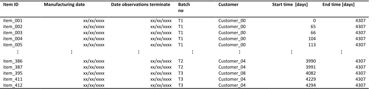
4.2.1 Items data-set

(8)

8

from records capturing failure occurrences. Table 2 shows some of the items in the data-set; their manufacturing date; the date the observations ended; the batch the item belongs to, which reflects different development standards; and the customer the item is assigned to. Most information was obtained from the AvionicSupp’s repair database excerpt. Unlike single sample failure data obtained in test rig conditions, it is common for field data that the

observation ceased before all possible failure events could be observed24. In this case, the

date the observations ended corresponds to the date the last entry was logged in the

FRACAS. This choice reflects the absence of better knowledge with regards to whether any item had been permanently discarded before such date.

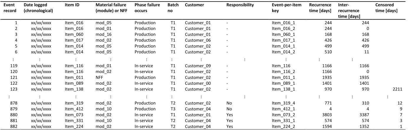
4.2.2 Failures data-set

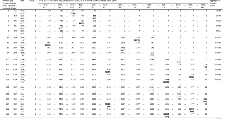
The ‘failure’ data-set provides recurrence data for multiple copies of a fielded repairable item. Table 3 shows some of the 1045 chronological logs of functional failures that have resulted in the removal of any copy of the LRI of interest. In the table, events logged on the same date for different items, or for different modules within the same item are reported on

separate lines. Failure events occurring on the last recording date are omitted42. It is worth

noting that an NFF occurring along with the detection of modules failure denotes a situation in which the malfunction originally suspected could not be confirmed and a different problem was detected, instead. Qualitative data in the free text fields of the FRACAS database were also explored to gain additional insight when data about which module failed or whether an NFF occurred were ambiguous, or absent. The values under the “recurrence times” and “interrecurrence times” headings were not part of the original data. Recurrence times were computed for each item as the difference between the date the event was logged and the item’s manufacturing date, which served as a proxy for the date the item was considered in-service. Hence, in Table 3 the recurrence times denote the item’s age at failure. Different items enter the in-service phase at different calendar dates, hence they are not considered at

risk of failing before such date. Such a situation is known as staggered entry23, or

left-truncation of lifetimes11. Due to the presence of staggered entries, the series of recurrence

times in Table 3 is not magnitude-ranked. Interrecurrence times are computed as the difference between successive recurrences for a certain item. Finally, a value under the “censoring times” heading indicates that the next recurrence time for an item is known to be greater than a certain value, but is not known exactly because the observation terminates before any additional event is recorded. Such a situation is commonly referred to as

(9)

9

censorings has dramatic repercussions in the choice of the analytical formulation of a model24, and ignoring it may lead to overly pessimistic reliability estimates28.

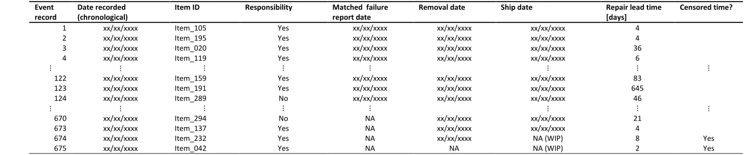
4.2.3 Repairs data-set

Table 4 shows some of the 512 chronological logs of actions completed in response to the reported functional failures of any LRI included in Table 2, the ‘repair’ data-set. Unlike the failure data-set, whether one or more modules were replaced or an NFF arose is indicated in the repair data-set aggregately on a single line, in a free text field. Hence, multiple lines in the failure data-set have only one line as a counterpart in the repair data-set. Analysis of the free text ensured consistency between the repair data-set and the failure data-set with regards to which modules had failed when the information was ambiguous. The “Removal date” provided a proxy date for events occurred after the last record in the FRACAS database.

The repair lead-time is computed as the difference between the outbound shipment date and the date the item is checked-in at AvionicsSupp (recording date). Most of the item-specific information contained in AvionicsSupp’s repair database is already shown in Table 1.

4.2.4 Data-sets alignment

The data-sets described above contain events about LRIs that are present in both JetProv’s FRACAS and AvionicSupp’s repair database. However, it was found that for certain LRIs some events were logged in FRACAS earlier than the manufacturing date. In the absence of additional information such a mismatch with regards to the events’ time origin reduced the number of useful records in the failure data-set to 867. After the update, the number of items for which at least one record existed in the failure data-set reduced to 362.

(10)

10

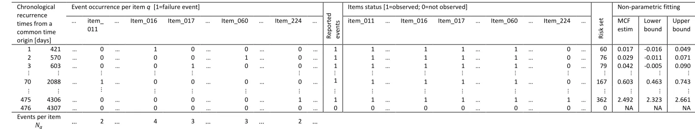
sample pattern of a stochastic process of point events in time. Such a layout is shown in Table 5 using a few items for illustrative purposes.

Table 5 HERE

Table 5 is obtained from Table 2 by complementing the use of spreadsheet with scripts

created in the open-source statistical computing language R43. The first column in Table 5

shows the chronologically ranked recurrence times obtained by superposing the recurrence times measured from the individual items’ time origin onto a common timescale. The time origin for such a timescale is the earliest date an item is fielded, hence the common timescale

measures the time-on-study rather than the items’ age11. Each recurrence time corresponds to

either a failure or an observation ceasing event, denoted respectively by 1 or 0 under the “status” heading. Hence, the times to non-failure recorded under the “censoring times” heading in Table 2 appear as additional lines in Table 5. Which item is affected by an event, at which age, and how long after the previous recurrence can be read column-wise.

For example, the first failure occurs at 421 days, when “Item_016” (affected) is aged 244 days, “Item_011” 268 days, “Item_014” 263 days etc. Observations for different items may start or stop at different times. At each recurrence the number of items observed, and hence be at risk of becoming a failure event, can be read under the “risk set size” heading in Table 5. For example, 60 items are in the risk set when the first failure occurs, whilst such items as “Item_073”, “Item089” etc. have not been fielded yet. Depending on which timescale is

chosen the risk set size, and the results of the analysis may change11. Multiple events

recorded on the same date for the same item in Table 2 (the lines with zero interrecurrence times) are skipped in Table 5. Information about which module failed, whether an NFF arose, etc. previously recorded on different lines in Table 2 is recorded on a single line in Table 5. It corresponds to the categorical explanatory variables that can be read column-wise. Multiple events logged on the same date for different items qualify as simultaneous failures but appear as separate lines. Simultaneous logs can be treated as distinct since they may be due to

coarseness in the timescale rather than genuine cascade-type failures44.

5 Findings

(11)

11

5.1 Failure data exploration

The data layout presented in Table 5 allows exploring reliability data for structure, especially

trends. Ascher26 has shown that “eyeball analysis” of a given set of times between successive

failures for a repairable item may be sufficient to reveal that failures are occurring more, less or as frequently, depending on their order. Fitting a parametric lifetime distribution to such failure times assuming a priori they are identically and independently distributed (i.i.d.) will cause the loss of such information.

In the presence of data obtained from multiple copies of fielded repairable items with

staggered entries and censoring times one should use aggregated times and number of failures

as shown in Table 5 to perform graphical and analytical tests for trends such as28:

 Plotting aggregate number of failures against the aggregated times. In the absence of

trend one would expect a plot that approximates a straight line; and

 Performing a Laplace (or centroid) test on the sequence of aggregate times. A positive

score, if significant, gives evidence that reliability deteriorates over time.

By using the case-specific figures partially shown in Table 5, one obtains the plot shown in Figure 2.

Figure 2 HERE

A visual inspection suggests that the slope of the plot increases over time. One can verify such trend analytically by using the Laplace test. A possible formulation of the test score for

𝑛 recurrence times 𝑥₁, 𝑥₂, … , 𝑥_𝑛 from the same time origin observed over a period of length

𝑡_𝑎, where 𝑡_𝑎 ≠ 𝑥_𝑛 is the following:

𝑈 =√12𝑛 𝑡_𝑎 (

∑𝑛 𝑥_𝑖

𝑖=1

𝑛 − 𝑡_𝑎

2) (1)

From the layout partially shown in Table 5, and considering only unique recurrence times

(𝑛 = 475 out of 624 failure events) one obtains: ∑𝑖=1𝑛 𝑥𝑖 = 231,279,108; 𝑡𝑎 = 833,526; and

𝑈 = 6.35. The test score is positive, and provides evidence that the interrecurrence times are tending

to become smaller – a situation colloquially known as a “sad” repairable item26_{. Such tendency is said}

to be statistically significant at 100𝛼% if 𝑈 exceeds the value 𝑧 such that 𝜙(𝑧) = 1 − 𝛼 2⁄ , where

(12)

12

Another graphical check for trends to plot autocorrelation coefficients between

interrecurrence times at different time lags, known as correlograms44. For the case considered

here, the coefficients are computed following Makridakis et al.45 up to 8 time lags, and are

shown in Figure 3.

Figure 3 HERE

Although it is not the case that all the coefficients are zero, as it would be expected from a

series of random numbers, all the values lie within the critical values ± 1.96 √𝑛⁄ = ±0.899

(𝑛 = 475) which seems to suggest ‘white noise’ data rather than a particular pattern.

Walls and Bendell44 suggest performing similar data exploration for repair times, too. In

principle, if considered as a set-of-number repair times can be treated analogously to failure times. Often, such terms as ‘failures’ and ‘repairs’ are used as synonyms to describe a generic

event of interest23. In the case of repairs, recurrence times are the items’ ages at completion of

each repair intervention. Hence, the time between successive recurrences is broader than the repair lead time.

Censoring times were found to affect repair times, too. In particular, there were entries in the repair database for which a date of completion was not yet available. Hence, the repair lead times for these interventions were not known, except for being greater than the difference between the repair log date and the date the observation terminated. In the absence of specific examples in the literature, trend analysis was performed as shown earlier, but using repair

completion times, where available, instead of failure times. The Laplace test score is 𝑈 =

−8.08 providing evidence of increasing repair times at 5% of statistical significance.

To rule out other elements that may affect the gap between two consecutive repair completion events, the same analysis was also performed using the lead times only, rather than the entire time between consequent repair completions. The corresponding Laplace test score is

𝑈 = −2.46, still negative and statistically significant.

5.2 Fitting models to data

Options for fitting models to empirical data can be parametric or non-parametric in nature, depending on whether or not they embed assumptions on certain features of the population

being studied23, 24. In the following sub-sections some of the options that are more appropriate

(13)

13

broad distinction is made between recurrence time models; interrecurrence time models; and regression models.

5.2.1 Recurrence times models

The preliminary data exploration suggests that, considering multiple copies altogether the LRI under investigation is a “sad” repairable item, hence, a model characterised by a

non-stationary (i.e., evolving over time) ROCOF should be fitted to the data26, 27. The main

parametric and nonparametric alternatives for the statistical analysis of recurrence data where recurrence times may not be i.i.d.are, respectively23:

 A population’s Mean Cumulative recurrence Function—MCF; and

 Point stochastic processes such as the Poisson process.

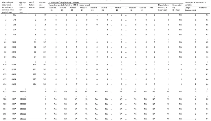
To illustrate the implementation of such models, the data layouts for the item data-set and the failure data-set are expanded as shown in Table 6 and Table 7 using a few selected items.

Table 6 HERE Table 7 HERE

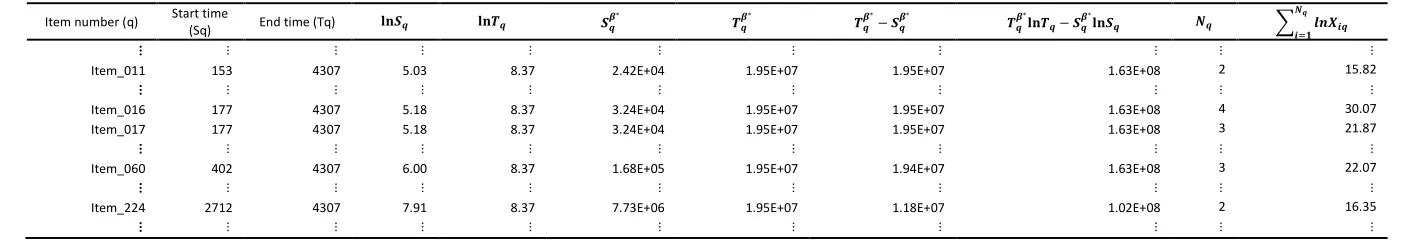
Table 6 presents additional columns compared to Table 2 which are necessary to estimate the parameters of a point stochastic process by numerical approximation, as shown later. Table 7 uses the same timescale as Table 5 to reflect staggered entries, however, it focuses on the unique times at which failure or observation ending events occur. At each unique recurrence time (row) and for each item (column) it is indicated whether the item is observed and part of the risk-set and whether it is affected by the failure occurrence.

Meeker and Escobar23 provide a detailed computational procedure to obtain a nonparametric

MCF estimator as the expected number of failures across a population of repairable items observed from individual time origins until failure, along with 95% confidence bounds. According to the procedure, at each unique recurrence time, ranked by magnitude, one computes the mean of the distribution of failure events experienced by the items that are in the risk set at that time. The non-parametric MCF estimator is then obtained by summing up the sample mean number of events up to that time. The relevant results are shown on the rightmost side of Table 7.

(14)

14

procedure was framed as shown in Figure 4 and implemented as a script for the computing language R.

Figure 4 HERE

In the algorithm, the vectors ‘reported.events’ and ‘riskset’ correspond to the ominous columns in Table 7, whilst the matrices ‘status.matrix’ and ‘events.matrix’ refer to the columns under the headings ‘Items status’ and ‘Event occurrence per item’ in Table 7.

Figure 5 shows graphically the estimated nonparametric MCF and 95% confidence envelope for the case considered here.

Figure 5 HERE

[image:14.595.159.485.599.714.2]

Since the model is nonparametric, to obtain a ROCOF one should divide the difference between the values taken by the MCF at successive times by the length of the time interval. Figure 5 also shows a parametric approximation which is typically recommended in the presence of trends: a non-stationary point stochastic process known as the Non Homogeneous

Poisson Process—NHPP26, 44.

One analytical formulation of the NHPP which is widely used in practice is the ‘power law’

NHPP, characterised by a non-constant ROCOF that is expressed as function 𝜈(𝑡, 𝜽) =

𝜆𝛽𝑡𝛽−1_{of time t and a vector}_{𝜽 = [𝛽, 𝜆]}_{of unknown parameters}23_{. The particular situation}

considered here is one in which recurrence data are obtained from 𝑘 copies of an item; each

item 𝑞(𝑞 = 1, … , 𝑘) is observed continuously from time 𝑆𝑞 to time 𝑇𝑞; during such period

each item experiences 𝑁_𝑞 failures, each failure 𝑖(𝑖 = 1, … , 𝑁_𝑞) occurring at a certain time

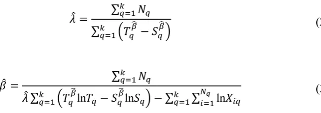
𝑋𝑖𝑞. In such a situation Crow46 expresses the maximum likelihood estimators of a power law

NHPP’s parameters 𝜆̂ and 𝛽̂ as the following set of equations:

𝜆̂ = ∑ 𝑁𝑞

𝑘 𝑞=1

∑𝑘 (𝑇_𝑞𝛽̂ − 𝑆_𝑞𝛽̂)

𝑞=1

(2)

𝛽̂ = ∑ 𝑁𝑞

𝑘 𝑞=1

𝜆̂ ∑ (𝑇_𝑞𝛽̂ln𝑇𝑞− 𝑆𝑞𝛽 ̂

ln𝑆𝑞) − ∑𝑘𝑞=1∑𝑁_𝑖=1𝑞 ln𝑋𝑖𝑞 𝑘

𝑞=1

(3)

Equations (2) and (3) are not in a closed form, but can be solved numerically with the aid of

(15)

15

arbitrarily chosen for 𝛽̂ on the rightmost side of equations (2) and (3). For example, 𝛽∗= 1

yields in our case ∑312_𝑞=1(𝑇_𝑞𝛽∗− 𝑆_𝑞𝛽∗)= 833,526; and ∑312(𝑇_𝑞𝛽̂ln𝑇_𝑞− 𝑆_𝑞𝛽̂ln𝑆_𝑞)= 7,349,788.4

𝑞=1 .

Considering that 𝑛 = ∑𝑘𝑞=1𝑁𝑞= 624 and ∑𝑘𝑞=1∑𝑁_𝑖=1𝑞 ln𝑋𝑖𝑞 = 5,003.2 one obtains 𝛽̂=1.25 form

equation (3). Ideally, the difference between 𝛽∗ and 𝛽̂ should be zero, but this might be unrealistic. Hence, the problem is to find a value 𝛽∗ > 0 such that the difference 𝑧 = 𝛽̂ − 𝛽∗_is

minimized subject to such a constraint as, for example 0 ≤ 𝑧 ≤ 0.000001. The value

𝛽∗= 2.012≅ 𝛽̂ which satisfies the constraints is found iteratively by using the Solver embedded in MS Excel®. The estimate obtained is greater than one, consistently with the

evidence of a “sad” item provided by the exploration of failure data for trend. Given 𝛽̂, one

obtains 𝜆̂= 1.217 × 10−7 from equation (2). The expected (mean) number of failures over a

time interval (0, 𝑡) is 𝐸(𝑁_𝑡) = 𝜆̂𝑡𝛽̂_{, and it is shown as a curve in Figure 5. The same analysis}

can be carried outdistinguishing between three different development standards (batches) of the LRI of interest, as shown in Figure 6.

Figure 6 HERE

In practical terms, the graphs shown in Figures 5 and 6 indicate the total number of functional failures resulting io a removal, that is experienced on average by an LRI over a certain time period. The underpinning function’s ROCOF is increasing which indicates that the time it takes, on average, an LRI to require an additional support intervention gets shorter the longer it has been in the field. This trend does not seem to by affected by the development standard a product belongs to.

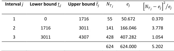
Crow46 provides a ‘goodness-of-fit’ statistic for the power law NHPP that is suitable when

the observations start time is not zero for all the item’s copies the data are obtained from:

 Identify at least 𝑚 = 3 time intervals, characterised in terms of upper and lower

bounds 𝑇_𝑗 = (𝑡_𝑗, 𝑡̅_𝑗)(𝑗 = 1, . . , 𝑚), containing at least five total failure occurrences;

 Compute the expected failures over each interval as 𝑒_𝑗 =𝜆̂𝑡̅_𝑗𝛽̂ − 𝜆̂𝑡_𝑗𝛽̂_{, where}_𝜆̂_and_𝛽̂

are the estimated parameters, and indicate the actual data number of failures as 𝑁_𝑇_𝑗;

 Compute the statistics 𝑋2 _{= ∑} _[𝑁

𝑇𝑗 − 𝑒𝑗]

2

𝑒_𝑗 ⁄

𝑚

𝑗=1 and compare it with the critical

value of a Chi-distribution (e.g., via lookup tables). Typically, 𝑚 − 1 degrees of

(16)

16

For the case considered here a critical value of 𝑋2 _{= 5.20}_{is obtained as shown in Table 8.}

Table 8 HERE

Its attained level of statistical significance, or p-value, from a Chi-distribution with 2 degrees of freedom is between 0.10 and 0.05, confirming the hypothesis that the observed values follow an NHPP with the estimated parameters.

5.2.2 Interrecurrence time models

As anticipated in Section 2, fitting parametric lifetime distributions is an appropriate way of modelling single sample data referring to items that fail only once, as in test rig conditions. However, this procedure is commonly applied to model repairable items, too, if there is no

strong evidence against the hypothesis of i.i.d. failure times47. Although the empirical data

considered here are characterised by the presence of trends, a complementary, distribution-fitting is of practical relevance, especially for estimating availability29. Also, it has been demonstrated that under certain circumstances the hazard functions of traditional lifetime

distributions can be used to model an NHPP’s ROCOF48.

When modelling the reliability of electronic products Weibull distributions are a common

choice12. However, to try to model the reliability of a repairable item by distribution-fitting

makes sense only if interrecurrence times are being analysed, since this amounts to

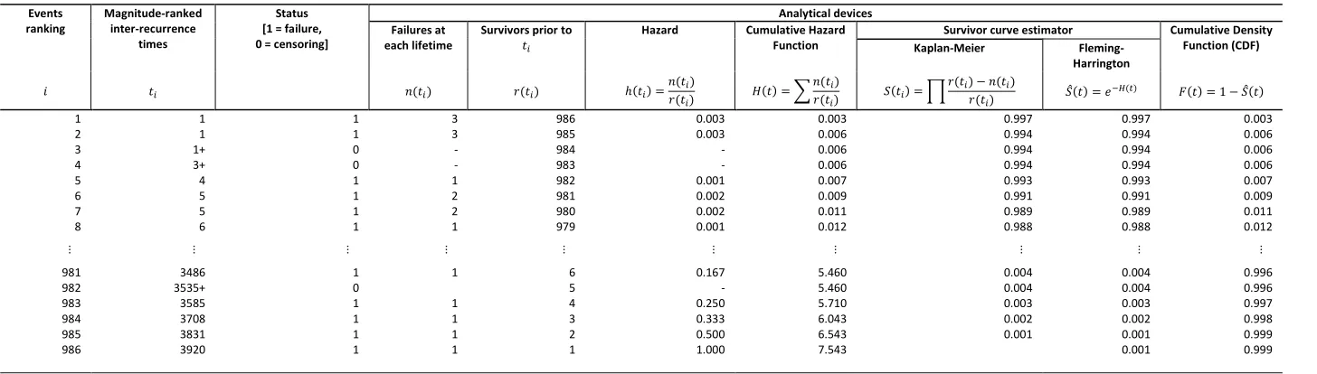
non-repairable component analysis28. One way to fit a Weibull distribution is by graphical

approach. The approach is based on magnitude-ranked interrecurrence times, and the estimation of their Cumulative Distribution Function (CDF) to obtain the coordinates of a

Weibull plot to which a straight line is fitted28. For the case considered here, there relevant

values and statistics are given in Table 9, and plotted as shown in Figure 7.

Table 9 HERE Figure 7 HERE

Unlike recurrence data analysis, the risk set in Table 9 is not the number repairable items being observed, but a number of fictitious non-repairable items which is equivalent to the number of failure events. From the slope and intercept of the line shown Figure 7 the estimators for the distribution’s shape and scale parameter are found to be, respectively,

𝛽̂_graph = 1 0.9915⁄ = 1.02 and 𝜃̂_graph = 𝑒6.658 _{= 731.15}_{. Another approach is to estimate}

the distribution’s parameter by maximum-likelihood. Venables and Ripley49 provide a robust

(17)

17

package for the statistical computing software R. Due to the presence of censoring times,

however, a modified version available in the “fitdistrplus” package50 has been used. The

interrrecurrence times and status data in Table 9 provide the inputs for the algorithm which

yields 𝛽̂_mle = 1.17 and 𝜃̂_mle = 1333.03. The empirical and estimated probability density

function (pdf) and cumulative distribution function (cdf) are shown in Figure 8.

Figure 8 HERE

A similar procedure can be carried out for each module rolled up in the LRI. For example, the module with most occurrences, “module_02” has a rather short characteristic life, expressed

by the scale parameter osrif the fitted lifetime distribution 𝜃̂mod_02 = 12.9 [days].

Finally, the lognormal distribution is often considered appropriate for modelling repair times29, 34. From the empirical data about repair lead times, the mean 𝜇̂_mle = 3.55 and

standard deviation 𝜎̂_mle = 1.15 of a lognormal distribution were estimated by maximum

likelihood using the “fitdistrplus” package for R. Figure 9 shows the empirical and estimated probability density function and cumulative distribution function.

Figure 9 HERE

The presence of censoring in the data prevents the straightforward application of testing procedures to assess the fit of the empirical data to the estimated distributions such as the

Kolmogorov-Smirnov (K-S) test. Modified K-S procedures for censored data are available51,

but only apply to the case in which censored observations are all greater than the largest observed value. In the absence of adequate alternatives, it is suggested to proceed by visually

inspecting the empirical and theoretical cumulative distribution functions50.

5.2.3 Regression models

A common trait of the models discussed above is that the items the data is gathered from are deemed indistinguishable. Especially when a large number of items is available for analysis heterogeneities (e.g., in configuration, operating conditions etc.) are known to affect the reliability of each copy. Regression type of analysis is appropriate in such a situation, and is less affected than other methods by such special conditions of reliability analysis as the

presence of censored data, and the arbitrary choice of lifetime distributions52. In particular,

the Cox ‘Proportional Hazard’—CPH model is a semi-parametric regression model of

survival analysis widely used in biometrics49, 52, with extensions that can be applied to the

(18)

18

determines how the hazard function varies from a common baseline between groups within the population being investigated by specifying explanatory variables that reflect the heterogeneous conditions under which data were collected. In the presence of variables the value of which may change over time for a given item—called time-dependent explanatory variables—an ‘extended’ Cox model, based on a layout in which each recurrence event is defined in terms of its ‘start’ and ‘stop’ time, is required11. For the case considered here the relevant explanatory variables are shown in Table 5. Some such variables, named ‘event-specific’, are inherently dependent whilst other, named ‘item-‘event-specific’, are

time-independent. The recurrence times in Table 5 serve as the ‘stop’ times, whilst the ‘start’ times can be obtained for each event for a given item by retrieving the previous event’s recurrence time. Once the empirical data are suitably arranged a Cox model for recurrence events can be

fitted via the “coxph” function provided with the survival package for R11, 49. By applying

this procedure one obtains regression coefficients corresponding to each explanatory variable included in the model and, for each such coefficient, a p-value for testing its significance and an Hazard Ratio (HR) for measuring the strength of the association between variables.

Statistically significant (p-values < 5%) associations were found for four modules

(“module_02”; “module_06”; and “module_10”), one customer (“customer_07”), and the phases the failure event occurs (coded as 1 for the in-service stage and 0 for production). The

estimated coefficients were, respectively: 𝛿mod_02 = −0.383; 𝛿mod_06 = −0.398; 𝛿mod_10 =

−0.749; 𝛿_{mod_14} = 1.338; 𝛿_{customer_07} = 0.715; and 𝛿_phase= −0.757. The interpretation of

such coefficients for inherently time-dependent explanatory variables is based on their HR11.

For example, the HR of the explanatory variable “phase” is 𝑒𝛿phase = 0.47_{, meaning that at}

any given time the hazard for an item which has not yet failed in-service (but may) is

approximately 1 0.47⁄ ≅ 2 times the hazard for an item which has already failed in-service

by that time. Similarly, the hazard for an item which has not yet experienced a material

failure in “module_02” at a given time is 1 𝑒_⁄ −0.383_{≅ 1.5}_{times the hazard for an item which}

has already experienced it by that time. By contrast, the customer variable is

time-independent. Hence, the value 1 𝑒_⁄ 0.757 _{≅ 0.5}_{means that the hazard for other customers is}

0.5 times the hazard for “Customer_07”.

5.3 Availability estimation

(19)

19

typically interpreted as the ratio of satisfactory operations to downtime, the most popular amongst the definitions given in Table 1 is static availability. Static availability is the limit of another function, called instantaneous or point availability also shown in Table 1.

Baxter29 provides an example of availability estimation from empirical data by numerical

evaluation of the following formulation of instantaneous availability:

𝐴(𝑡) = 𝐹̅(𝑡) + 𝐹̅(𝑡) ∗ ∑∞ 𝐹𝑛_{(𝑡) ∗ 𝐺}𝑛_(𝑡)

𝑛=1 (4)

where 𝐹(𝑡) is the distribution function corresponding to the interrecurrence times’ pdf; 𝐺(𝑡)

is the distribution function corresponding to the repair lead times’ pdf; 𝐹̅(𝑡) = 1 − 𝐹(𝑡) is the

probability that the item functioned without failure up to time t.

At the heart of equation (4) is an operation called Stieljes convolution, denoted by the operator “*”, of two distribution functions which yields the distribution function of the sum of the two underlying random variables. Superscript “n” in equation (4) denotes the n-fold

recursive convolution of a certain distribution function. Baxter29 suggests using cubic splines

approximations of the function to be convoluted. Ruckdeschel and Kohl53 provide a generic

algorithm for R to execute the convolution between two distributions based on Fast Fourier Transforms. Although such concepts may sound familiar to the mathematically literate, it was felt by the authors that the implementation of such approaches, although still possible via “black boxes”, would have required dealing with theories which go beyond the scope of this

paper. A more pragmatic approach to the evaluation of equation (4) described by Mullineux54

and implemented as shown in Figure 10 was chosen.

Figure 10 HERE

The algorithm divides the abscissa into a series of intervals of equal width h (e.g., 1). It employs R built-in commands to evaluate the estimated pdfs and cdfs over the discrete timeline t thus obtained (e.g., for the Weibull distribution function such commands are

“pwebiull” and “dweibull”, respectively). A subroutine named “deriv.approx(A)” is employed

to approximate the derivative of a generic function 𝐴(𝑡) evaluated along t by numerical

differentiation, that is, by computing the slope of a nearby secant line through two points. Another subroutine called “convolve.trapez(A, b)” performs the Stieljes convolution between

(20)

20

function 𝑏(𝑡) = 𝑑𝐵(𝑡)_𝑑𝑡 is preliminarily obtained via the “deriv.approx(A)” subroutine already

mentioned. Then, 𝐴(𝑡 − 𝑢) and 𝑏(𝑢) are evaluated and the results multiplied. Finally, the

integral of the function defined by the sequence of numbers thus obtained is computed in a simplified way by approximating the area underneath the function as a trapezoid. Both subroutines are described concisely as algorithms in the Appendix.

To evaluate equation (4) for the case considered here, the focus was on those subsets of the repair and FRACAS datasets that overlap. In such a way it was possible to associate each repair intervention on a certain item with the uptime that followed, measured as the difference between the outward shipping date and the next date a failure was logged in for that item. In this case, the interrecurrence times are identified with the uptimes only, not with the whole difference between two consecutive recurrence dates. Also, censored

interrecurrence times arise in those situations in which a repair intervention is known to be completed beyond the last recorded event in the failure database, but before the last recorded event in the repair database. Finally, by focusing only on the matched failure and repair events it was possible to compute ‘empirical’ availability as the number of items no failed a certain number of days after each completed repair.

Figure 11 shows the point availability function estimated applying the algorithm in Figure 10 to the matched failure and repair data (solid line); the point availability function obtained from all the available data (dashed line); and the empirical availability at each ‘time after repair completion’.

Figure 11 HERE

When using the matched failure and repair data, the function 𝐴(𝑡) appears to remain close to

its asymptote lim𝑡→∞𝐴(𝑡) ≅ 0.981 after roughly 502 days. When using all data, instead, the

function settles down to a limiting value of 0.949 at roughly 2,424 days. The limiting value, or “static availability”, can be computed also directly in a relatively straightforward way once the estimated pdfs’ parameters are known.

For example, knowing that the expected (mean) values of the estimated failure and repair

times’ pdfs estimated in the previous section are, respectively, 𝜇₁ = 1260.96 and 𝜇₂ = 67.49

(21)

21

6 Discussion

The implementation of a specific strategy for the analysis of empirical data obtained from fielded items is an often overlooked aspect. The theoretical grounds for such a strategy are touched in principle by nearly any reliability engineering handbook. However, in the

presence of a limited number of practical examples and applications to real-life case studies it is not always clear how one should proceed when the incumbent ways to go about reliability data analysis do not apply. Such aspects range from organising empirical data in a suitable layout, through their preliminary exploration, to the identification and implementation of alternative formulations of a model to be fitted to the data.

The importance of the data layout is seldom treated explicitly and in sufficient detail.

Kleinbaum and Klein11 offer extensive discussion with regards to the survival analysis of

recurrent events. Meeker and Escobar23 give examples for the non-parametric MCF

estimator. An appropriate data layout accommodates the presence of censored data, including both right-censoring, and the staggered entry into service of different copies of an item. Such an aspect is often neglected when it comes to practical implementation since works make almost without exception the assumption that recurrence times are measured from a common

origin. Newton28 is amongst the few authors demonstrating how insidious this can be. The

“methods” section of this paper has dealt with obtaining ‘data-sets’ form the raw company-provided data, rather than focusing directly on a ‘set-of-numbers’ deprived of context.

The preliminary exploration of the empirical data is acknowledged as a necessary step to prevent the uncritical acceptance of the hypothesis that the sequence in which failure events occur is of no importance. The Laplace or centroid test is mentioned, amongst others, in most

handbooks23, 42. Newton28 provides indication on how to proceed in the presence of multiple

copies, staggered entries and censored data. In practical applications, however, whether a choice is made for modelling the reliability of a repairable item as an NHPP or by fitting some parametric distribution to recurrence data is not grounded on empirical data

exploration. Either no test is performed on the available data17, 22 or, if performed, such tests

typically lead conclude that no structure is identified18, 47. This results in a lack of practical guidance on how to interpret and follow up the results of preliminary data exploration.

(22)

22

treated as two facets of the same coin—some “relevant” event—in the statistical analysis of

recurrence data23. To the authors’ knowledge, they are typically not subject to separate

analyses. In the absence of further guidance, it was chosen to fit a parametric recurrence time model, and a non-parametric recurrence time model to failure recurrence data only.

Non-parametric recurrence times models such as the MCF estimator are seldom applied to

case studies. An exception is Bumblauskas et al.55, who present a case study in electric power

equipment. However, the use of a specific software package for reliability analysis does not allow a detailed discussion on how staggered entries were dealt with. Hence the choice was

made here to implement the algorithm in Meeker and Escobar23 from first principles. The

MCF plots were used to compare items from different design developments. Regardless the group the items belong to, evidence seems to be against reliability growth. The power-law NHPP was chosen as the parametric recurrence time model. Its most popular analytical

formulations is a closed form which assumes a single item only17, 26. If multiple copies of an

item are considered, it tends to be assumed they have the same observations’ start and end

time22. In the case considered here, the non-closed form equations that apply in all other

cases, which are characteristic of field reliability data, have been chosen, and numerically solved using resources available in common electronic spreadsheets.

In practical terms, recurrence time analysis via MCF or power-law NHPP provides insights into good and poor performing items in the field that can be filtered by model years,

development standard, production lot numbers etc. One may be interested, for example, in which model years within an installed base have performed well to identify best practices, or which ones performed poorly to identify whether a design review is needed. A word of caution, however, is necessary. A product design review might show increased reliability under the test rig conditions. Yet, as Figure 6 shows, it is not the case that product design reviews alone can be expected to affect the total number of support interventions demanded, on average, by an LRI once fielded. In such cases insight into the whole socio-technical support system including maintenance practices is necessary. For example, a previous case study employing interviews demonstrated that differences in the maintenance philosophy between different aircraft led to coding analogous LRI removal events differently, as an NFF in one case and as a repair in another, thus affecting the quantitative analysis’ results13.

(23)

23

the most common probability distributions to data are available, the presence of censoring times requires careful selection of which procedure to apply. Despite its importance, such an aspect remains mostly unaddressed in case studies where probability distributions are the

model of choice for empirical data18, 29, 47. Also, the assessment of the goodness-of-fit of the

estimate obtained considering censored times is still problematic, except for a particular kind of right-censoring which mostly occurs in test rig conditions.

Semi-parametric regression models for recurrence data were also considered as an

appropriate way to overcome the simplifying assumption that multiple copies of a fielded item are identical, as well as dealing with censored recurrence times. Applications of such an approach to repairable systems under fixed-price maintenance and repair contracts include

Lugtigheid et al.56. However, the existing application provides little practical guidance since

the chief purpose of using a Cox’s PH model was that of estimating the intensity function of a power-law NHPP rather (a practice which can be controversial in the light of the discussion

in Ascher27) than as an autonomous model. Also, no mention of the ‘modified’ Cox model

which may be necessary when the explanatory variables are time-dependent (and hence the ‘proportionality’ assumption the PH model relies on no longer holds) is made. In the case presented here, both time-dependent and time-independent explanatory variables were identified, and this required particular attention to the interpretation of the results of the Cox model fitted to the empirical data.

Finally, the estimation of availability from empirical data appears to be extremely rare, rather, most academic works focus on the theoretical refinement of availability modelling and on

simulation12. In any case, availability estimation requires known probability distributions of

failure and repair times as a starting point. The need to follow one of the few procedures for

the numerical evaluation of point availability29 has diverted the attention towards parametric

lifetime distribution rather than to models of recurrence data that are deemed appropriate for repairable items. Also, such operations as convolution and derivations had to be approached pragmatically to avoid introducing mathematical concepts that are seldom applied within the scope of the analysis presented in this paper. Visualising empirical data against an estimated theoretical point availability function as in Figure 11 is not common practice, and required focus on a subset for which failure and repair data matched. In the electricity supply industry it is common for companies to report metrics such as the System Average Interruption Duration Index (SAIDI) which expresses the average duration of outages experienced per

(24)

24

theoretically to determine an optimal inventory policy for transformer assets, by adopting the common assumption of a constant failure rate upfront. Since the theoretical availability results thus obtained are not linked with empirical data, their usefulness for drawing conclusions on real-life problems is limited.

7 Conclusion

In this paper, a strategy for the statistical analysis of field reliability data has been outlined and applied to a case study underpinned by real-life data in defence avionics. Some ‘forgotten lessons’ in field reliability data analysis have been identified and taken into account

throughout as a guidance for improving the understanding of reliability baselines. Especially for the effective execution of availability-based contracts, field reliability data analysis is an essential step towards a defensible attribution of operational unavailable time to the

organizations involved. However, incumbent practices in reliability engineering seem to hinder the analyst’s ability to choose between available modelling options based on an intelligent exploration of data ‘in context’.

The research presented in this paper has devoted particular attention to providing data with context. The expected benefit is to allow practitioners to appreciate the differences between models that are meant for non-repairable items, such as parametric lifetime distributions, and those meant for repairable items that, by contrast, focus on a sequence of times to failures. Such aspects as organising data according to an appropriate layout; the preliminary

exploration of data for trends; and the need to deal with the presence of staggered entries and right-censored data have been considered. Such aspects are often taken for granted although they can have major repercussions on the models of choice as well as the most adequate analytical formulation of such a model. Although it is acknowledge that increasingly sophisticated analytical functionalities are offered by reliability engineering software

packages, it appears that in the implementation of such functionalities common assumptions remain largely concealed and hence not questionable by practitioners.

(25)

25

evident through the application of each model to the specific case study. The need for

industrial practice of approaching reliability baselines with more awareness of the diversity of methods of analysis available in the literature, rather than chasing some ideally truest, ‘one-size-fits-all’ solution is perhaps most effectively expressed in the words of Evan’s:

“We all use models all the time. We use them, not because they are great, but in spite of their being lousy […] All we can ask of our models in any of these situations is that the

model we are using be adequate for the purposes at hand”59.

Even if an appropriate model is selected the uncritical interpretation of the model’s results may trigger tension between suppliers, manufacturers, and customers/end users. In the context of availability contracting, a superficial interpretation of a model’s outcomes may lead to undesirable outcomes from breaches in contract terms and conditions, which can in turn lead to litigation. Future research should support a more constructive use of the results obtained from field reliability data analysis as a basis on which different stakeholders can build through collaboration the necessary agreement underpinning performance and quality improvement.

This research has limitations mainly due the absence of detailed guidance from previous applications of models other than those prescribed by the incumbent practices. In the absence of such guidance the researchers have experienced difficulties in the identification,

application and interpretation of models and their analytical formulation that seemed more adequate to reflect the context of the data at hand. Examples include the implementation of a non-closed form of the equations to estimate a power-law NHPP’s parameters; and the

difficulties of providing a goodness-of-fit statistic for probability distributions in the presence of censored data.

Another limitation of the analysis is that the focus was deliberately confined on models for which guidance on the use of empirical field reliability data commonly gathered by industry was available, rather than attempting to comprehensively cover theoretical refinements. As a consequence, the approaches presented were almost exclusively time-based. Although it can be argued that a focus on time as the only relevant independent variable in reliability analysis is always appropriate, alternative modelling approaches for equipment maintenance support,

(26)

26

It was beyond the scope of this research to employ the models fitted to the data to make predictions regarding the case study at hand. As most other words, the statistical analysis of field reliability data presented here provides a retrospective analysis of ‘parts that broke’. A word of caution seems necessary with regards to drawing conclusions about such a complex system as the enterprise executing an availability contract from the analysis in hindsight of

the some of the physical components involved. As Dekker61 has observed, a technology that

may appear tidy on the drawing board can easily turn out to be unruly once it hits the field, thus undermining the predictive power of retrospective analysis.

References

1. Zio E. Reliability engineering. Old problems and new challenges. Reliability

Engineering & System Safety 2009;94:125-141.

2. Baines T, Lightfoot H. Made to serve. How manufacturers can compete through servitization and product-service systems. Wiley: Hoboken, NJ, 2013.

3. BAE Systems. BAE Systems wins £446M Typhoon contract, 2012.

http://www.baesystems.com/article/BAES_045629/446m-typhoon-contract-will-help-sustain-600-uk-jobs [Oct 15, 2014].

4. Smith TC. Reliability growth planning under performance based logistics. In

Proceedings of the Annual Reliability and Maintainability Symposium 2004;418-423. 5. Hollick LJ. Achieving shared accountability for operational availability attainment. In Proceedings of the Annual Reliability and Maintainability Symposium 2009;247-252. 6. Candell O, Karim R, Soderholm P. eMaintenance-Information logistics for maintenance

support. Robotics and Computer-Integrated Manufacturing 2009;25:937-944.

7. Meier H, Uhlmann E, Krug C, Völker O, Geisert C, Stelzer C. Dynamic IPS2 networks and operations based on software agents. CIRP Journal of Manufacturing Science and

Technology 2010;3:165-173.

8. Rees JD, van den Heuvel J. Know, Predict, Control: A Case Study in Services

Management. In Proceedings of the Annual Reliability and Maintainability Symposium 2012;1-6.

9. Simões JM, Gomes CF, Yasin MM. A literature review of maintenance performance measurement: A conceptual framework and directions for future research. Journal of

Quality in Maintenance Engineering 2011;17:116-137.

(27)

27

11. Kleinbaum DG, Klein M. Survival Analysis. A self-learning text. Springer: New York, 2012.

12. Sandborn P. Cost Analysis of Electronic Systems. World Scientific: Singapore, 2013. 13. Blackwell P, Hausner E. The redefinition of supportability and its role as a systems

engineering tool. Naval Engineers Journal 1999;111:269-277.

14. Wong KL. The bathtub does not hold water any more. Quality and Reliability

Engineering International 1988;4:279-282.

15. Pecht MG, Nash FR. Predicting the reliability of electronic equipment. Proceedings of

the IEEE 1994;82:992-1004.

16. Kumar DU. New trends in aircraft reliability and maintenance measures. Journal of

Quality in Maintenance Engineering 1999;5:287-295.

17. Crespo Márquez A, Parra Márquez C, Gómez Fernández J, López Campos M, González-Prida Díaz V. Life Cycle Cost Analysis. In Asset Management, Van der Lei T, Herder P, Wijnia Y (eds). Springer: Amsterdam 2012;81-99.

18. Waghmode L, Sahasrabudhe A. Modelling maintenance and repair costs using stochastic point processes for life cycle costing of repairable systems. International Journal of

Computer Integrated Manufacturing 2012;25:353-367.

19. Held M, Fritz K. Comparison and evaluation of newest failure rate prediction models:

FIDES and RIAC 217Plus. Microelectronics Reliability 2009;49:967-971.

20. Hauptmanns U. Reliability data acquisition and evaluation in process plants. Journal of

Loss Prevention in the Process Industries 2011;24:266-273.

21. Bowman RA, Schmee J. Pricing and managing a maintenance contract for a fleet of

aircraft engines. Simulation 2001;76:69-77.

22. Weckman GR, Marvel JH, Shell RL. Decision support approach to fleet maintenance

requirements in the aviation industry. Journal of Aircraft 2006;43:1352-1360.

23. Meeker WQ, Escobar LA. Statistical methods for reliability data. Wiley: New York, NY, 1998.

24. Phillips MJ. Statistical methods for reliability data analysis. In Handbook of reliability engineering, Pham H (ed). Springer: London 2003;475-492.

25. Evans RA. Stupid statistics. IEEE Transactions on Reliability, 1999;48:105.

26. Ascher H. Discussion of "point processes and renewal theory: a brief survey". In

(28)

28

27. Ascher HE. A set-of-numbers is NOT a data-set. IEEE Transactions on Reliability,

1999;48:135-140.

28. Newton DW. Some pitfalls in reliability data analysis. Reliability Engineering & System

Safety 1991;34:7-21.

29. Baxter LA. A case study in availability forecasting. Microelectronics Reliability

1985;25:927-942.

30. Sikos L, Klemeš J. Evaluation and assessment of reliability and availability software for securing an uninterrupted energy supply. Clean Technologies And Environmental Policy

2010;12:137-146.

31. Yellman TW. Failures and related topics. IEEE Transactions on Reliability, 1999;48:

6-8.

32. Rijsdijk C. Predicting availability. Maintworld 2013;5:24-26.

33. Reich P. Problems in the investigation of reliability-associated life-cycle costs of military airborne systems. In Methodology for control of Life Cycle Costs for avionic systems. AGARD/NATO: Neuilly-sur-Seine CEDEX, 1979;5.1-5.21.

34. Blanchard BS. Logistics engineering and management. Prentice-Hall: Englewood Cliffs, NY, 1992.

35. BS EN IEC 60300-3-16:2008 Dependability management. Application guide. Guide to the specification of dependability requirements. BSI: London, 2009.

36. Rai RN, Bolia N. Availability-based optimal maintenance policies for repairable systems in military aviation by identification of dominant failure modes. Proceedings of the Institution of Mechanical Engineers, Part O: Journal of Risk and Reliability

2014;228:52-61.

37. Settanni E, Thenent NE, Newnes LB, Parry G, Goh YM. A strategy for field reliability data analysis for use in performance-based support contracts. Manuscript submitted for publication.

38. BS EN IEC 60300-3-16:2008 Dependability management. Application guide. Guidelines for specification of maintenance support services. BSI: London, 2009.

39. Curry EE. STEP: a tool for estimating avionics life cycle costs. IEEE Aerospace and

Electronic Systems Magazine, 1989;4:30-32.

40. Kiang T. The development and implementation of Life Cycle Cost methodology. In Methodology for control of Life Cycle Costs for avionic systems. AGARD/NATO: Neuilly-sur-Seine CEDEX: 1979;3.1-3.25.

(29)

29

42. O'Connor PD. Practical reliability engineering. Wiley: Chichester, 1991.

43. R Development Core Team. R: A Language and Environment for Statistical Computing, 2012. Vienna, Austria. http://www.R-project.org/.

44. Walls LA, Bendell A. The structure and exploration of reliability field data: What to

look for and how to analyse it. Reliability Engineering 1986;15:115-143.

45. Makridakis SG, Wheelwright SC, Hyndman RJ. Forecasting. Methods and applications. Wiley: New York, 1998.

46. Crow LH. Evaluating the reliability of repairable systems. In Proceedings of the Annual Reliability and Maintainability Symposium 1990;275-279.

47. Tsarouhas PH. Reliability Analysis into Hospital Dialysis System: A Case Study.

Quality and Reliability Engineering International 2013;29:1235-1243.

48. Krivtsov VV. Practical extensions to NHPP application in repairable system reliability

analysis. Reliability Engineering & System Safety 2007;92:560-562.

49. Venables WN, Ripley BD. Modern applied statistics with S. Springer: New York, NY, 2007.

50. Delignette-Muller ML, Dutang C. Fitting parametric univariate distributions to non censored or censored data using the R fitdistrplus package.

http://www.icesi.edu.co/CRAN/web/packages/fitdistrplus/vignettes/intro2fitdistrplus.pdf [October 15, 2014].

51. D'Agostino RB, Stephens MA. Goodness-of-fit techniques. Dekker: New York, NY, 1986.

52. Ascher H. Regression analysis of repairable systems reliability data. In Electronic Systems Effectiveness and Life Cycle Costing, Skwirzynski JK (ed). Springer-Verlag: Berlin Heidelberg, 1983;119-133.

53. Ruckdeschel P, Kohl M. General Purpose Convolution Algorithm in S4-Classes by

means of FFT. Journal of Statistical Software 2010;59:1-25.

54. Mullineux G. Discretized distributions notes: FCALC. Unpublished manuscript. University of Bath, Department of Mechanical Engineering, 2014.

55. Bumblauskas D, Meeker W, Gemmill D. Maintenance and recurrent event analysis of circuit breaker data. International Journal of Quality & Reliability Management

2012;29:560-575.

56. Lugtigheid D, Jardine AKS, Jiang X. Optimizing the performance of a repairable system under a maintenance and repair contract. Quality and Reliability Engineering

(30)

30

57. IEEE 1366-2003. Guide for Electric Power Distribution Reliability Indices. IEEE: New York, NY, 2004.

58. Mielczarski W, Khan ME, Sugianto LF. Management of inventory to reduce outages in supply feeder. In Proceedings of International Conference on Energy Management and Power Delivery 1995;222-227.

59. Evans RA. Models Models Everywhere - And Not A One To Want. IEEE Transactions

on Reliability, 1995;44:537.

60. Bender A, Pincombe AH, Sherman G. D. Effects of decay uncertainty in the prediction of life-cycle costing for large scale military capability projects. In Proceedings of the 18th World IMACS / MODSIM Congress 2009;1573-1579.

(31)

31