Towards data centric control of sensor networks through Bayesian dynamic linear modelling

Towards data-centric control of sensor networks

through Bayesian dynamic linear modelling

Lei Fang

School of Computer Science University of St Andrews, UK

Email: [email protected]

Simon Dobson

School of Computer Science University of St Andrews, UK Email: [email protected]

Abstract—Wireless sensor networks usually operate in dy-namic, stochastic environments. While the behaviour of indi-vidual nodes is important, they are better seen as contributors to a larger mission, and managing the sensing quality and performance of these missions requires a range of online decisions to adapt to changing conditions. In this paper we propose an self-adaptive, self-managing and self-optimising sensing framework grounded in Bayesian dynamic linear models. Experimental results show that this solution can make sound scheduling decisions while also minimising energy usage.

Index Terms—self-management, adaptive sampling, sensor net-works, machine learning, energy efficiency

I. INTRODUCTION

Wireless sensor networks (WSNs) offer several motivating challenges for self-organising systems. A typical objective of a sensor deployment is to sample an environment at a desired pace and send the observations back to a “sink” location. The whole process needs to take energy efficiency into account. Centralised control has been the dominating approach in the literature where either management decisions are made at the sink or some top-down co-ordination is used. Although these solutions have only lightweight local computation, they suffer from scalability problems and potentially a single point failure. More importantly, the power used in node-server communica-tion might outweigh the power saved through minimising local computation.

A bottom-up, self-organising solution is therefore desirable. Ideally one would like local decisions to be made indepen-dently, with little (or no) communication overhead. A globally optimal result might not be achieved this way: but “good” results should be expected if sound local decisions are made. As a data-driven application, sensor nodes need to under-stand a certain extent of the physics which they are tasked to measure in order to achieve well-founded local control. This is not always straightforward. Firstly, the physics is usually very hard to model. Specific models do exist for some applications, such as flooding or meteorology. However, these models are usually too complicated to be included at sensor level, and also too specific to be reusable in other more general settings.

Secondly, the physics is fundamentally uncertain and is further confused by measurement error, outside perturbations that go unobserved, the (often unavoidable) degradation of sensor ca-pabilities over time, and the impact of management decisions such as energy-saving on sensor fidelity.

Understanding and addressing these issues requires that we adopt a management approach that is grounded both in the engineering of sensor networks and in the behaviour being observed. One approach is to use machine learning to track observations and make control decisions in response. While machine learning is often too heavyweight to be deployed on compute-constrained nodes, there are approaches that are appropriate for such settings.

In this paper, we explore Bayesian Dynamic Linear Models (DLM) as an approach to local decision-making that can take place at an affordable cost. DLMs tailored to general sensor platforms together with the efficient model inference procedures are derived. The benefits of employing DLMs are their formal basis in Bayesian inference; their general-ity; their robustness to missing and perturbed observations; and their distribution efficiency that allows for purely local implementation. To put the model into use, we investigate the practical-sampling scheduling problem where each sensor node decides autonomously when to sample and how the data can be recovered. We show how DLM inference allows sensor nodes to decide the sampling time locally, and that a globally “good” result can be achieved out of this bottom-up, self-organising design: all the results are achieved without any form of centralised liaison. The paper concludes with further applications and benefits of using DLMs, and some notes for the future.

II. RELATEDWORK

problem and single point failure. Another paradigm also called replicated models solution features keeping synchro-nised models both at the sink and network. PAQ [2], [3], for example, employs an autoregressive (AR) model for sensor data modelling. However, ARIMA model usually requires computational intensive learning phase; moreover, the learning cannot be done on-line. Low-Energy Adaptive Clustering Hier-archy (LEACH) [4] and Adaptive Sampling Approach to Data Collection (ASAP) [5] fall into the category of cluster-based in-network aggregation method. The cluster based solutions usually require some form of intra-cluster co-ordination, and the overhead on cluster head node could be significant.

Regarding sampling control, some similar solutions have been put forward. An decentralised adaptive sampling control method is proposed in [6] where Fisher Information and Gaus-sian process (GP) regression are used. The solution targets at a specific application with specialised hardware platform that can handle intensive learning task of GP. Other similar solutions include [7], where the authors present a utility-based adaptive sampling solution. A piecewise linear function is used to model the sensor data. But the model learning requires storing of the learning data locally, and the model update is not straightforward. A prediction-based geometric data stream monitoring solution is proposed in [8]. The solution aims at reducing sink-node communication. However, the solution tar-gets at triggering event detection where a non-linear function of the distributed data source is of interest.

III. BAYESIANDYNAMICMODELLING

Bayesian Dynamical Linear Models (DLMs) have been successfully applied in analysing financial time series [9], [10], and some others like medicine, ecology data [11], [12]. How-ever, the close linkage between DLMs and sensor platforms has not been well discovered. In this section, the backbone of the proposed solution: DLMs is introduced with a focus on its connection with sensors.

A. Model Definition

Sensor data can be viewed as a collection of (multivariate) time series; let yit, a p-variate vector, denote the sensor data

measured at time t by node i; then Yi = {yi

t, t ≥ 1}

represents the time series collected by node i. A dynamic linear model is a probabilistic time series model which can be formulated as follows (node idiis dropped for convenience):

Definition 1 (Bayesian Dynamic Linear Model).

Sensor model: yt=Ftθt+vt, vt∼Np(0,Σt) (1a)

Process model: θt=Gtθt−1+wt,wt∼Nm(0,Ωt), (1b)

together with a prior forθ0

θ0∼Nm(m0,C0); (1c)

where Gt (of order m×m) and Ft (p×m) are scalar

matrices,Np(µ,Σ)denotes ap-variate Gaussian distribution with mean and covariance matrixµand Σ respectively, and

vt,wtare independent to each other for all t.

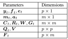
The dimensions of the relevant parameters are summarised in Table I.

TABLE I

PARAMETERS OF ADLMMODEL Parameters Dimensions yt,ft,et p×1

mt,at m×1

Ct,Rt,W,Gt m×m

Qt,V p×p

Ft p×m

A DLM can be completely specified by a quadruple:

{Ft,Gt,Σt,Ωt},

plus the initial prior parameters {m0,C0} for θ0, where

Ft and Gt are usually fixed matrices that depend on the

model of choice; however the two covariance matricesΣtand

(especially) Ωt, the unobserved state evolution variance, are

unknown.

B. DLM for sensors (univariate)

A DLM model suits the sensor context particularly well. Equation (1b), which is a first-order Markovian stochastic process, can be actually viewed as the model for the hidden physical phenomenon of interest (for example temperature). The model assumes the physical process is stochastically evolving over the time and its current state depends on its previous state subject to some linear transformation Gt and

some stochastic small changes wt. Intuitively, this process

assumption is appropriate for most physical variables: for instance, the current temperature develops upon its previous state plus some small change either positive or negative. Equation (1a) represents the sensor or observation model, where sensor measurements yt are formed by “observing”

the hidden processθt, again plus some unbiased observation

errors. Figure 1 shows the DLM definition graphically: the round nodes represent the hidden physical process whose value depends on its previous state; while the square nodes are the sensor observations of the corresponding hidden process.

θ0 θ1 θ2 θ3 θ4

y1 y2 y3 y4

1) process model assumption for sensors: The legitimacy of the process model can be further established as follows. Assume the physical process can be formed as a real-valued continuous function of time, say, φ(t). Note the assumption applies to most sensor settings. The process then can be modelled by setting θt as an m-component random vector

(with the corresponding Ft = (1,0, . . . ,0)′ and Gt as a m×m upper triangular matrix of unit elements), leading to the m-order polynomial trend DLM. For example, a second-order polynomial DLM (also called local linear trend model, hereafter referred to as simply trend model) is formed with a hidden state θt= (µt,βt)′, and

yt=µt+vt, vt∼N(0,σv2), (2a) µt=µt−1+βt−1+wt,1, wt,1∼N(0,σw,2 1), (2b)

βt=βt−1+wt,2, wt,2∼N(0,σw,2 2), (2c)

which is equivalent to a DLM with the following settings:

Ft:=E= [1 0], Gt:=L=

!_{1 1}

0 1 "

,

andwt= (wt,1, wt,2)′,Ωt=diag(σw,2 1,σ2w,2).The model can be simplified by setting Ωt = σ2

v ·diag(Wt,1, Wt,2), where Wt,i = σw,i2 /σ2v is the corresponding variance ratio. Define Wt =diag(Wt,1, Wt,2), the corresponding model quadruple

is

M2: [E,L,σ2v,Wt]. (2d)

Other DLMs with different orders can be formed similarly, although in real world data analysis only the first two orders are relevant. To see the connection between the model and the physical process φ(t), apply the Taylor expansion toφ(t) at time ti: the function atk-unit time step forward can then be

written as

φ(ti+k)≈φ(ti) +φ′(ti)k+. . .=

∞ #

n=0 ˜

φ(in)kn,

where φ˜(_in) = φ(n)_(t

i)/i!1. The m-order polynomial DLM

actually corresponds to the m-order Taylor expansion of the physical process function with φ˜(_in) matches the (n+ 1)th element of θt, where the unknown polynomial coefficients

˜

φ(in) are stochastic and subject to random noise rather than

being fixed. For most sensor data, linear approximations (i.e. 1st- or 2nd-order DLMs) are sufficient to capture the future evolvement of the process; higher order models with complicated polynomial growth are usually not appropriate unless that specific growth is knowna priori.

1_{This argument holds as long asf is continuous and differentiable}

C. Multivariate DLM extension

For most WSN applications the deployed nodes have more than one type of sensor, and the intra-node variates are usually correlated. Figure 2, for example, shows temperature and humidity observations that are negatively correlated. To model multivariate sensor data, an easy extension could have been treating yi,t for i ∈ {1, . . . , p} as independent components.

However, this extension ignores the inter-variate correlations and also excludes the important “borrowing strength” of the multivariate model.

A more realistic model can be built based upon the univari-ate DLMs. Assume each univariunivari-ate sensor data yi,t admits a

polynomial DLM model (i.e. local level or trend model):

yi,t=Ftθi,t+vi,t, vi,t∼N(0,σii2); (3) θi,t=Gtθi,t−1+wi,t, wi,t∼Nm(0,Wtσii2). (4)

The multivariate model can be constructed as follows:

yt= (Ft⊗Ip)θt+vt, vt∼Np(0,Σ); (5a) θt= (Gt⊗Ip)θt−1+wt. wt∼Nmp(0,Wt⊗Σ), (5b)

where yt = (y1,t, . . . , yp,t)′, vt = (v1,t, . . . , vp,t)′, In

is a n-order identity matrix, ⊗ is the Kronecker product,

Σ= (σ2

ij)p×p is the (symmetric, positive-definite) covariance

matrix ofvt; andθt=vec(Θt′),wt=vec(Ω′t), where Θt= (θ1,t, . . . ,θp,t), Ωt= (w1,t, . . . ,wp,t),

and vec is the standard vec-operator which stacks the columns of am×pmatrix into ampcolumn vector. This multivariate DLM model still conforms to the general DLM definition, with a modified quadruple

[Ft⊗Ip,Gt⊗Ip,Σ,Wt⊗Σ]. (5c)

Among the four elements, only Σ, and Wt are unknown

(whose learning algorithm is discussed in the next section). The inter-variate correlation is introduced by the measurement covariance Σ: e.g. off-diagonal covariances with larger mag-nitude indicate a stronger linkage between the two variates.

To summarize, with the help of the above formalisms, various sensor data, univariate or multivariate, can be modelled by first selecting the appropriate univariate DLM quadruple and then transforming it to a multivariate model by (5).

38.8 39.0 39.2 39.4

18.0

18.5

19.0

Humidity (%)

T

e

m

p

e

r

a

t

u

r

e

(

°

C

)

(a) Node 1

39.4 39.8 40.2

18.0

18.5

19.0

19.5

Humidity (%)

T

e

m

p

e

r

a

t

u

r

e

(

°

C

)

(b) Node 2

Fig. 2. The intra-node attributes correlation: humidity versus temperature

Relying on the distributions, informed decisions about future data collection can be made.

For a DLM with a known quadruple, the seminal Kalman filter [13] can be used to estimate the predictive distribution. However, in real sensor applications, the covariance matrices of the quadruple are unknown until the data is actually observed. Traditional maximum-likelihood estimation might be used [14]: however, such estimation requires an iterative optimisation procedure.

Instead, we use conjugate Bayesian learning that treats unknown quantities as random variables to achieve an afford-able inference engine. To simplify the illustration, only the multivariate DLM result is presented; however, the univariate case can be easily recovered as a special case. To achieve this computational efficiency, the conjugate prior for{Σ,θ0} (the unknown quantities of a DLM2_{) is assumed. An}

Inverse-Wishart (IW) distribution is the natural conjugate prior dis-tribution for (matrix valued) variance. There exist different IW distribution functions in the literature [15], [16], [17], [9], [18]: in this paper, we adopt the definition used in [17]:

Σ∼IW(ν,S)with density

p(Σ)∝C×|Σ|−(ν+p+1)/2_exp $

−1

2tr(SΣ −1₎

%

,

where C=&

2νp/2_πp(p−1)/4'p

i=1Γ &ν+1−i

2 ((−1

· |S|−ν/2 _is a constant that is independent of Σ3.

Theorem 1 (Bayesian conjugate learning). Adopt the

follow-ing prior distribution for θ0,Σ|∅:

p(θ0,Σ) =p(θ0|Σ)p(Σ) =N(m0,C0⊗Σ)IW(n0,S0) (6)

!N IW⊗(m0,C0, n0,S0) (7)

2_{Efficient specification ofW}

t is detailed in the following section

3_{Quintana [19] and West [12] use a different form of IW which lead to}

different estimation update rules forν andS. The benefit of our definition is that the estimation algorithm for S is completely recursive and can be calculated without re-scaling.

for some pre-determined parameters m0,C0, n0,S0 in the multivariate sensor DLM model specified in(5).

for t >0:

1) Evolution stept:

θt|Σ,y1:t−1∼Nmp(at,Rt⊗Σ)

where

at= (Gt⊗Ip)mt−1, Rt=GtCt−1G′t+Wt (8a)

2) Conditional predictive:

yt|Σ,y1:t−1∼Np(ft, QtΣ),

with unconditional predictive

y_t|y_1:t−1∼Tp(f_t, QtSt−1 nt−1−p+ 1

, nt−1−p+ 1)

where

ft= (Ft⊗Ip)at, Qt=FtRtF′t+ 1 (8b)

3) Updated Posterior att:

θt,Σ|y1:t∼N IW⊗(mt,Ct, nt,St),

with marginal

Σ|y_1:t∼IW(nt,St)

where

mt=at+ (Kt⊗Ip)e′t, Ct=Rt−KtK′tQt,

nt=nt−1+ 1, et=yt−ft

Kt=RtF′t/Qt, St=St−1+ete′t/Qt

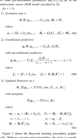
(8c) Figure 3 shows the Bayesian learning procedures graphi-cally. Without concrete prior knowledge, the prior is usually set diffusive or non-informative. Note the posterior distribution is adapted or learnt when more data is admitted; and the diffusive prior is shrinking as more data is learnt. In this work, non-informative priors are always used. According to Theorem 1, the predictive distribution is ap-variate Student T distributed. A Student T is similar to a Gaussian distribution but with heavier tail. The following useful results are listed. First, any subset of a multivariate T-random vector is still Student T distributed with model parameters immediately available from the joint distribution. This result allows one to infer on each individual sensor observation without any further computational effort.

Result 1 (Marginal T Distribution). Let x =

!

x1

x2 "

be

dis-tributed as Tp(µ,Σ,ν) withµ= !

µ1

µ2 "

, Σ= !_Σ

11 Σ12

Σ21 Σ22

"

and |Σ22|>0, whereµ1andµ2arep1,p2 dimensional ran-dom vectors andp1+p2=p. Then the marginal distribution,

xi,i= 1,2, is also T distributed; Specifically,

xi∼Tpi(xi;µi,Σi,ν).

Second, the conditional distribution, on the other hand, provides a more informed distribution that takes inter-variate correlations into account. For example, when partial observa-tion x2 is available, the conditional distribution onx1can be obtained by:

Result 2 (Conditional T Distribution). The conditional

distri-bution,x1|x2, isp1-variate T distributed:

x1|x2∼Tp₁(x1;µ1|2,Σ1|2,ν1|2),

where

ν1|2=ν+p2 (9a)

µ_1|2=µ₁+Σ12Σ−122(x2−µ2) (9b)

Σ1|2=

ν+ (x2−µ2)TΣ−122(x2−µ2)

ν+p2

&

Σ11−Σ12Σ−122Σ21(.

(9c) Note the conditional distribution is essentially an update upon the marginal densities where the “update” is provided by the partial observation.

A. Specification of Wtby Discount Factor

Theorem 1 only works whenWtis pre-specified. In reality,

the matrix that represents the variance ratios also needs to be learnt from data. Unfortunately, this complicated model (with essentially two unknown variance matrices {Σ,Wt}) has no closed form solution [14]. To resolve the problem, we adopt the common practice of specifying Wt dynamically as

a discount factor of Pt=GtCt−1G′t, Wt= 1

−δ

δ Pt, (10)

whereδ∈(0,1]is the discount factor selected by the modeller [12], [9], [20]. δ actually represents the percentage of the precision lost astincrements. For routine analysis,δis usually selected between the range [0.9,0.99] [12]; in this work, a

δ = 0.9 is used. We adopt the method not only because it achieves good forecasting results but also there is no need to store Wt specifically, as it is implicitly defined by Pt,

an existing parameter used in Theorem 1. This “parsimony” property is important for sensor nodes with limited storage capacity. The following theorem shows that the Bayesian conjugate analysis with discount factor specification is efficient in both a time and a space sense.

Theorem 2. For a DLM model(5)with unknownΣand

dis-count factor specification ofWt, the algorithm in Theorem 1

has constant O(1) space complexity and linear O(n) time

0 50 100 150

22

23

24

25

26

time

Filter

ing le

vel estimates

Sensor Observations DLM Filtering Hidden State 90% Filtering Interval

−10 0 10 20 30

0.00

0.05

0.10

0.15

0.20

0.25

Temperature

Density

t=0 t=1 t=4 t=8 t=32

Fig. 3. Bayesian conjugate inference with a noninformative prior

complexity, where nis the point the update stops or the size of the time series.

Proof. Note the recurrent relationship between (8a) and (8c): there is no need to store at,Rt specifically as they can

be updated directly upon {mt−1,Ct−1}. At each time in-stance t, the procedures require the exact local storage of

et,ft,Qt,Kt,St, n, and no historic sensor data need to be

stored; therefore, the space complexity is constant at each time instance. For time complexity, we calculate the complexity of each step in Theorem 1: at eacht, (8a) is ofO((mp)2_+m3_); (8b) is ofO(p×mp+m2_{); (8c) is ofO(m}2_+mp×p+m2_+p2_); the total isO((mp)2_+m3_+mp2_{) =O(max(m, p)}4_{). Note} when a DLM is chosen, m, p are both constant integers: therefore the time complexity is constant at each t, leading to a linear growth astincrements.

B. Model update with missing observation

Sensor nodes are unreliable, not only in the sense that sensor observations might be faulty, but that they may not be available from time to time. In both cases, the rational practice is to treat the observation as missing. Fortunately, model update with missing observation can be performed easily with Bayesian learning. To deal with a missing observation at t – so yt is

missing – one simply adopts the following update procedures to replace Equation (8c):

mt=at;Ct=Rt;nt=nt−1;St=St−1; (11a)

the procedures follow becausep(θt,Σ|y1:t−1,yt=NULL) = p(θt,Σ|y1:t−1), the new observation provides no real update to the model. At the(t+ 1)th evolution step after the update step, the following evolution procedure is adopted instead of Equation (8a):

at+1= (Gt+1⊗Ip)mt, Rt+1=Gt+1CtG′t+1+Wt,

0 20 40 60 80 100

0.6

0.8

1.0

1.2

Sensor data

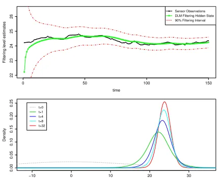
Sensor Observations DLM Forecast 90% Forecast Interval

Fig. 4. Filtering when observation are missing

where Wt= 1_δPt is the previous evolution matrix specified

at t. Note the update actually maintains a constant step-ahead evolution matrix, Wt+1 = Wt. This modification

prevents the explosion of the evolution variance Rt when

multiple k consecutive observations are missing. To see this, if {yt+1:t+k} are missing, the ordinary evolution step (8a)

would lead to

Rt+k =GkCtGk′/δk,

where Gk ! Gt+kGt+k−1· · ·Gt+1. Since δ lies in (0,1],

Rt+k will increase exponentially as k accumulates, which

contradicts the linear form of DLM [12]. Figure 4 demon-strates graphically the model update procedures with missing observations. Note the forecast interval (model uncertainty) automatically adjusts when data is missing.

h-step-ahead forecast: Theorem 1 provides the algorithm for calculating the one-step-ahead forecast distribution. The general h-step-ahead forecast distribution with h > 1 can actually be easily obtained by treating the future observations

{yt+1:t+h−1} as missing. The result is true because the following identity

p(yt+h|y1:t) =p(yt+h|y1:t,yt+1:t+h−1=null). (12) V. SENSORCONTROL WITHDLM

To show the practical use of DLM, we investigate the sampling scheduling problem of WSNs. An DLM based data collection framework featuring adaptive sampling and guaranteed sampling accuracy is proposed and evaluated in this section. The framework forms a self-organizing distributed solution where each node determines locally the sampling decisions with the help of DLMs and global good results can be achieved out of this self-managed scheme.

A. Problem Statement

Let ϵ be the precision required of the sensor data. For example, if the true signal is s ∈ R, then any value within the range of [s−ϵ, s+ϵ] is satisfactory. The problem is to determine the sampling time for each sensor node such that

the sampled and collected data meet the precision requirement with small computational overhead. As pointed out by Alippi et al. [21], the energy spent on sensing is comparable to other intensive sensor activities including RF communication. However, blindly reducing sensing will lead to insufficient samples, which in turn results in inadequate data collection. Therefore, the trade-off between accuracy (resolution) and energy efficient needs to be resolved by the autonomic control.

B. Overview

The proposed solution starts with a one-offmodel learning phasein which each sensor node learns its local DLM model according to Theorem 1 until a pre-determinedNlnumber of

sensor observations have been learnt or the model parameters have stabilised. To ease the computation burden for the sensor nodes, only univariate DLM models are maintained for each sensor data series. For the convergence test, we examine the prediction’s variance

Λt= QtSt−1

nt−1−p+ 1

and stop the learning phase if

|Λt−Λt−1|

Λt−1 <0.01.

The objective of this phase is to obtain a functioning DLM model with learnt and stabilised model parameters. Note that to communicate the learned result, the nodes are not required to send back the learning data to the sink but only the posterior model parameters. After receiving the model parameters, the sink has the synchronised DLM models maintained in the network.

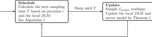
The operational phase commences after the learning phase. Figure 5 shows the procedures in the operational phase graph-ically. Each node first decides the next sampling time, T, by making inference on the DLM model. The sampling schedule decision is made such that only those “valuable” or “interest-ing” samples are taken, and the rest is lost during the period in between. The nodes then act according to the sampling schedule: upon time T, the node takes a series of Iupdate

Schedule

Calculate the next sampling

timeTbased on precisionϵ

and the localDLM;

See Algorithm 1

Update

SampleIupdatereadings;

Update the localDLMand

server model by Theorem 1

Sleep untilT

Fig. 5. Dynamical linear model based data collection framework flow chart

C. DLM Based Sampling Scheduling

According to Theorem 1 and (12), an h-step ahead predic-tion distribupredic-tion is still Student T distributed:

yt+h|y1:t∼T(f(h), Q(h),ν(h)).

Therefore, a prediction interval can be derived:

P)f(h)−tα,ν(h)

*

Q(h)<

yt+h< f(h) +tα,ν(h) *

Q(h)+= 1−2α, (13) where tα,ν(h) is the critical percentile value for the Stu-dent T random variable. For example, when α = 2.5% is used, the future observation yt+h will fall in the envelope

,

f(h)−t0.025,ν(h) *

Q(h), ft(h) +t0.025,ν(h) *

Qt(h)

-with a 95% level of confidence, conditional on all the historic data. As hrolls forward, the uncertainty accumulates so the in-terval expands. In view of this, a sensor node applies a greedy algorithm to decide when to sample again: as long as the confidence interval is smaller than the user-specified precision interval [f(h)−ϵ, f(h) +ϵ], there is no motivation to sample the environment as the future observations are likely with high confidence to be within the forecast interval; meanwhile its precision is also satisfactory. Algorithm 1 summarises this scheduling decision making procedure.

Algorithm 1 Sampling scheduling greedy algorithm

Input: Precision ϵ (ϵ > 0); Forecast limit H; Forecasting

confidence levelα

1: h←1

2: whileh≤H do

3: Calculate Q(h),ν(h)based on Theorem 1 and (12)

◃Calulate the h-step ahead prediction interval 4: if tα,ν(h)

*

Q(h)>ϵthen

5: break outer while loop

6: end if

7: h←h+ 1

8: end while

9: T ←h−1

D. Model Update

Upon the scheduled sampling point T, the sensor node reaches the model update stage, in which the node samples the

environment and updates the local model again. This update stage is necessary as the accumulating uncertainty has reached a threshold such that model inference cannot satisfy user’s precision requirement.

We denote the sampling size asIupdate, i.e. at T the sensor node takesIupdate consecutive samples. These sensor readings need to be reported back to the sink so that both the local node and the sink update their DLM models according to The-orem 1.Iupdatemay be defined by the user as a fixed constant. However, it can also be determined dynamically on an on-demand basis: the update stage finishes when the predictive interval shrinks and falls below a threshold, say the user-defined precisionϵagain.

E. Data restoration at the sink

For data collection applications, the sink needs to report all the sensor measurements for end users. This means the sink needs to recover those missing observations that were not taken due to the adaptive sampling policy.

With the DLM formalism, the data restoration can be achieved with little computational effort. Assume observation

yt is missing. Since the local and server models are always

synchronized during the update phase; therefore, the sink can simply supply the one-step-ahead point forecast ft from

Theorem 1 as the missing values for each of the univariate DLM it maintains. In other words, the missing values are replaced by ft = Eyt|y_1:t₋₁[yt]. Note it can be shown that the point forecast has the smallest expected squared loss,

Eyt|y_1:t₋₁[(yt−ft)

2_{] =}. _(y

t−ft)2p(yt|y1:t−1)dyt,

which means the estimator has the smallest squared dis-crepancy between the missing observation according to the posterior distribution, making it the best estimator for the missing valueyt.

An alternative method is to train an additional multivariate DLM model out of the received but incomplete data so that the cross sectional correlations can also be used to interpolate the missing data. The multivariate DLM learning result Theorem 1 can be used to learn the model. Since each univariate DLM is operated independently; therefore, the received data might happen to complement each other: at each time instance t:

1) the whole observation vectory_tis missing; or

2) some subsetyt,1 of it is missing while the restyt,2 are observed, whereyt= (yt,1,yt,2)′;

To summarize, apart from the data transmission during the model update phase, there is no other server-sensor commu-nication is required. First, the scheduling decisions are self-determined at each local sensor node; and the data restoration at the server works purely on the data already received without any further query from the sensors. Therefore, the solution is indeed bottom-up and self-organizing.

VI. EVALUATION

We present an evaluation in two parts. Firstly we show that the update procedures can all be feasibly implemented on a platform of the capabilities typically used for sensor networks. Secondly, we simulate the behaviour of our system against commonly-used trace data. We defer evaluation of a deployment in the wild to future work.

A. Implementation

To demonstrate the algorithm is a feasible solution for resource constrained sensors, we have implemented the frame-work in nesC on TinyOS 2.1.0 [22] and evaluated it using IEEE 802.15.4 complaint TMote Sky mote. It consists of an processor running at maximum 8MHz and RAM of 10 KB [23]. The relative small RAM size becomes a major hindrance for the system and application program. The pro-posed solution with two univariate DLM models embedded (assumed to be temperature and humidity) is implemented. The implementation has a footprint of 584 RAM (in bytes) and 21432 ROM (in bytes), which only account for5.7%and 43.6%of the total size.

B. Simulation Results

We drive our simulations from sensor data collected as part of a real-world deployment [24]. The simulation is written in R [25] and the results reported are summarized over ten independent runs with sensor data series (temperature, humidity and voltage sensors) randomly selected from the data set. Our method is assessed from two aspects: data collection accuracy, and communication saving. The former assessment shows the quality of the autonomously made decision; the latter demonstrates how sensor nodes can benefit from the sound decisions. We compare the results against the fixed rate sampling schedule which is currently the most widely used scheduling solution regarding the two aspects.

1) Assessment on decision making: To assess the autonomic control, we examine the quality of the collected data that is sampled based on the DLM enhanced scheduling algorithm. Two metrics,Mean Absolute Difference(MAD) andPrecision Satisfactionare used. The metrics are defined as

Mean Absolute Difference= 1

N N

#

i=1

|d˜i−di|, (14)

Precision Sat.= / /

/{d˜i :|d˜i−di|<ϵ, i∈1, . . . , N} / / /

N , (15)

wheredi, d˜i are the original data collected according to the

fixed rate sampling schedule and the data collected as per the sampling scheduling respectively. MAD shows the average difference between the data, while precision satisfaction shows the percentage of the collected data is satisfactory towards the user’s requirement.

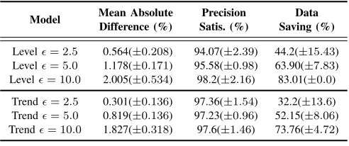
Tables II to IV show the results for temperature, humidity and voltage data respectively. Two DLM models, 1st (level model) and 2nd (trend model) order polynomial DLMs, are considered. For each type of sensor, we report the simulation results on different levels of precision ϵ requirements. The reported results are the averages together with the standard deviations over the ten independent runs. The following ob-servations can be made based on the tables.

• First, for all the different settings, the mean absolute

difference achieved are below their precision requirements: which means on average the decisions made satisfies the application’s requirements. It is also interesting to note the solution adapts itself well to the user’s precision require-ments. When a demanding data precision is required, the solution delivers the performance as required, which can also be seen graphically from Figure 6.

• Second, all the precision satisfaction entries are around

95% (if ± the standard deviation). The high satisfaction rates imply the decisions made in general are sound and satisfactory. Recall a 95% credible interval is used in the simulation, the results roughly matches our expectation, which also means the DLMs are reliable in delivering the forecasts.

• Third, the trend model outperforms the level model

coun-terparts in data quality for most of the settings. However, the difference on voltage is negligible. This is due to the fact that the voltage data is more stable than the other two data (it does not grow or decline randomly); therefore, a local level model without stochastic trend component is sufficient to model its dynamics.

• Forth, the effect of multivariate DLM based server side

data restoration is also apparent from the results. The spatial correlations between the temperature data is ex-ploited to construct a multivariate DLM model at the sink. According to Table II, both the MAD and precision satisfaction are improved by the multivariate extension. Note the multivariate restoration makes use of the same amount of data as the univariate restoration; therefore, they have the same energy saving as the univariate case.

• Last but not least, the proposed solution works on all the

TABLE II

SIMULATION RESULTS ON TEMPERATURE SENSOR DATA

Model Mean Absolute Difference (°C) Precision Satisfaction (%) # of Data Data

Univariate Multivariate Univariate Multivariate Messages Saving (%)

DLM-Levelϵ= 0_.3 0.086(±0_.01) 0.0682(±0_.01) 93.94(±1_.39) 95.4(±2_.39) 5841.4(±196_.5) 59.4(±1_.36) DLM-Levelϵ= 0.5 0.114(±0.017) 0.07(±0.01) 95.96(±0.59) 97.6(±2.51) 5364.4(±260.8) 62.8(±1.81) DLM-Levelϵ= 1.0 0.217(±0.037) 0.15 (±0.051) 96.5(±1.16) 97.7 (±2.50) 3776.7(±69.12) 73.8(±0.48) DLM-Trendϵ= 0_.3 0.062(±0_.009) 0.047 (±0_.007) 95.7(±1_.13) 96.7 (±3_.93) 6274.3(±270_.78) 56.4(±1_.88) DLM-Trendϵ= 0.5 0.079(±0.015) 0.054 (±0.012) 96.9(±0.91) 97.9 (±2.52) 5899.4(±121.4) 59.0(±0.84) DLM-Trendϵ= 1.0 0.167 (±0.033) 0.125 (±0.21) 96.8(±0.82) 98.1 (±2.43) 5295.5(±74.03) 63.2(±0.51)

Time

Or

iginal Data

0 2000 4000 6000 8000

18

20

22

24

26

Time

Le

vel epsilon =1.0

0 2000 4000 6000 8000

18

20

22

24

26

Time

T

rend epsilon =0.3

0 2000 4000 6000 8000

18

20

22

24

26

Fig. 6. Evaluation of the DLM-based solution on temperature sensor data. The top figure shows the original data; the middle frame is the data collected by the level model withϵ = 1_{°C; the bottom frame is the result for level}

model withϵ= 0_.3°C.

TABLE III

SIMULATION RESULTS ON HUMIDITY SENSOR DATA

Model Mean Absolute Precision Data

Difference (%) Satis. (%) Saving (%)

Levelϵ= 2_.5 _0.564(±0_.208_{) 94.07(±}2_.39_{) 44.2(±}15_.43₎

Levelϵ= 5_.0 1.178(±0_.171) 95.58(±0_.98) 63.90(±7_.83) Levelϵ= 10.0 2.005(±0.534) 98.2(±2.16) 83.01(±0.0)

Trendϵ= 2_.5 _0.301(±0_.136_{) 97.36(±}1_.54_{) 32.2(±}13_.6₎

Trendϵ= 5_.0 0.819(±0_.136) 97.23(±0_.96) 52.15(±8_.06) Trendϵ= 10.0 1.827(±0.318) 97.6(±1.46) 73.76(±4.72)

TABLE IV

SIMULATION RESULTS ON VOLTAGE DATA

Model Mean Absolute Precision Data

Difference (%) Satisf. (%) Saving (%)

Levelϵ= 0_.01 _0.002(±0_.002_{) 94.3(±}3_.19_{) 47.5(±}25_.86₎

Levelϵ= 0_.03 _0.007(±0_.001_{) 96.3(±}1_.63_{) 91.5(±}0_.76₎

Levelϵ= 0_.05 0.007(±0_.001) 98.5(±1_.54) 91.8(±0_.0) Trendϵ= 0_.01 _0.002(±0_.002_{) 94.6(±}2_.71_{) 47.9(±}25_.3₎

Trendϵ= 0_.03 _0.007(±0_.001_{) 96.4(±}1_.81_{) 91.5(±}0_.79₎

Trendϵ= 0_.05 0.007(±0_.001) 98.4(±1_.6) 91.8(±0_.0)

2) Assessment on communication saving: According to Ta-bles II to IV, it is clear that for all three types of sensors, the proposed solution significantly reduces the data communica-tion in comparison with the original solucommunica-tion. For example, for the temperature sensor at a precision requirement level of

ϵ = 0.5°C, the amount of actual data communication of the local level model is 5364.4 messages, and the corresponding saving is over 62.8%, which means over 62% of the original data is exempted from sending back to the sink. Similar results can be found for the other two sensors. It is interesting to see how the solution adaptively responds to the different settings of the precision requirement. In general, when the less precise data is required, the solution saves more on data communication.

VII. CONCLUSION

In this paper, we put forward the use of Bayesian dynamic linear models for local sensor node control. DLMs are general models that can capture the physical context, which provides valuable information for the local node to make informed deci-sions. More importantly, lightweight learning algorithms exist such that all the model inferences can be done independently at local sensor node level without any form of inter-node co-ordination or centralized control.

APPENDIXA PROOF OFTHEOREM2

Proof. An indirect proof is to show the equivalence of (5) and the Matrix Normal Dynamic Linear Model (MNDLM) developed in [18]. However, due to the different specifications of IW, the estimation rules would diverge slightly; a direct proof is given below. By Kalman Filter theory, the estimation rules forat,ftfollows, as (5) is still a DLM.

(1) Evolution step:Var[θt|Σ,y1:t−1] = (Gt⊗Ip)(Ct−1⊗

Σ)(Gt⊗Ip)′+Wt⊗Σ= (GtCt−1G′t⊗Σ) +Wt⊗Σ=

(GtCt−1G′t+Wt)⊗Σ=Rt⊗Σ.

(3) Prediction step: the variance of the conditional distribu-tion,QtΣ, can be proved by the same way as step one except Qt⊗Σ = QtΣ as Qt is a scalar. The unconditional result

follows due to the property of Normal Inverse Wishart [17]. (3) Update step: denote the precision matrixΛ=Σ−1; by Bayes’ theorem:

p(Σ|y1:t)∝p(Σ|y1:t−1)p(yt|y1:t−1,Σ))

∝|Λ|(nt₋₁+p+1)/2

exp{−tr(St−1Λ)/2}

|Λ|1/2exp0

−(yt−ft)′Qt−1Λ(yt−ft)/2

1

∝|Λ|(nt₋₁+p+1+1)/2

exp{tr(ete′t/Qt·Λ) +tr(St−1Λ)} =|Λ|(nt₋₁+p+1+1)/2

exp{tr(StΛ)}∝IW(nt,St),

which proves the update procedures for Σ. The update rules for θtcan be proved by noting

!

θt yt

"/ / / /

y1:t−1,Σ∼N !!

at ft

"

,

!

Rt⊗Σ RtF′t⊗Σ FtR′t⊗Σ Qt⊗Σ

"" ;

apply Gaussian regression theory [26],

θt|Σ,y_1:t∼Nmp(mt,Ct⊗Σ)

is proved.

The above are valid for allt >0, which proves the theory. REFERENCES

[1] A. Deshpande, C. Guestrin, S. R. Madden, J. M. Hellerstein, and W. Hong, “Model-driven data acquisition in sensor networks,” in Pro-ceedings of the Thirtieth international conference on Very large data

bases - Volume 30, ser. VLDB ’04. VLDB Endowment, 2004, pp.

588–599.

[2] D. Tulone and S. Madden, “PAQ: Time series forecasting for approxi-mate query answering in sensor networks,” inWireless Sensor Networks. Springer, 2006, pp. 21–37.

[3] Y.-A. Le Borgne, S. Santini, and G. Bontempi, “Adaptive model se-lection for time series prediction in wireless sensor networks,”Signal

Processing, vol. 87, no. 12, pp. 3010–3020, 2007.

[4] M. J. Handy, M. Haase, and D. Timmermann, “Low energy adaptive clustering hierarchy with deterministic cluster-head selection,” in

Mobile and Wireless Communications Network, 2002. 4th International

Workshop on. IEEE, 2002, pp. 368–372. [Online]. Available:

http://ieeexplore.ieee.org/xpls/abs all.jsp?arnumber=1045790

[5] B. Gedik, L. Liu, and P. S. Yu, “ASAP: An Adaptive Sampling Approach to Data Collection in Sensor Networks,”Parallel and Distributed

Sys-tems, IEEE Transactions on, vol. 18, no. 12, pp. 1766–1783, 2007.

[6] J. Kho, A. Rogers, and N. R. Jennings, “Decentralized control of adaptive sampling in wireless sensor networks,” ACM Transactions

on Sensor Networks (TOSN), vol. 5, no. 3, p. 19, 2009. [Online].

Available: http://dl.acm.org/citation.cfm?id=1525857

[7] P. Padhy, R. K. Dash, K. Martinez, and N. R. Jennings, “A utility-based sensing and communication model for a glacial sensor network,” in

Proceedings of the Fifth International Joint conference on Autonomous

Agents and Multiagent Systems, 2006, pp. 1353–1360.

[8] N. Giatrakos, A. Deligiannakis, M. Garofalakis, I. Sharfman, and A. Schuster, “Distributed geometric query monitoring using prediction models,” ACM Trans. Database Syst., vol. 39, no. 2, pp. 16:1–16:42, May 2014. [Online]. Available: http://doi.acm.org/10.1145/2602137 [9] C. M. Carvalho and M. West, “Dynamic matrix-variate graphical

mod-els,”Bayesian Analysis, vol. 2, no. 1, pp. 69–98, 2007.

[10] J. Quintana, V. Lourdes, O. Aguilar, and J. Liu, “Global gambling,”

Bayesian Statistics, 2003.

[11] C. Calder, M. Lavine, P. M¨uller, and J. S. Clark, “Incorporating multiple sources of stochasticity into dynamic population models,” pp. 1395– 1402, 2003.

[12] M. West, R. Prado, and A. Krystal, “Evaluation and comparison of EEG traces: Latent structure in nonstationary time series,”

Journal of the American Statistical . . ., 1999. [Online]. Available:

http://www.tandfonline.com/doi/abs/10.1080/01621459.1999.10474128 [13] R. E. Kalman, “A new approach to linear filtering and prediction

problems,” Journal of Fluids Engineering, vol. 82, no. 1, pp. 35–45, 1960. [Online]. Available: http://fluidsengineering.asmedigitalcollection. asme.org/article.aspx?articleid=1430402

[14] G. Petris, S. Petrone, and P. Campagnoli,Dynamic linear models with R. New York, NY, USA: Springer, 2009.

[15] A. K. Gupta and D. K. Nagar, Matrix variate distributions. Boca Raton, FL: CRC Press, 1999, vol. 104. [Online]. Available: http: //books.google.com/books?hl=en&lr=&id=PQOYnT7P1loC&pgis=1 [16] A. P. Dawid, “Some matrix-variate distribution theory: Notational

con-siderations and a Bayesian application,”Biometrika, vol. 68, no. 1, pp. 265–274, 1981.

[17] A. Gelman, J. B. Carlin, H. S. Stern, and D. B. Rubin,Bayesian data

analysis. New York, NY, USA: Chapman & Hall, 2014.

[18] M. West and J. Harrison, Bayesian forecasting and dynamic models. New York, NY, USA: Springer, 1997.

[19] J. M. Quintana, “Multivariate Bayesian forecasting models,” Ph.D. dissertation, University of Warwick, Mar. 1987. [Online]. Available: http://webcat.warwick.ac.uk/record=b1452026$\sim$S1

[20] H. Migon and D. Gamerman, “Dynamic models,”

Hand-book of Statistics, vol. 25, pp. 553—-588, 2005.

[Online]. Available: http://hedibert.org/wp-content/uploads/2013/12/ migon-gamerman-lopes-ferreira-2005.pdf

[21] C. Alippi, G. Anastasi, C. Galperti, F. Mancini, and M. Roveri, “Adaptive Sampling for Energy Conservation in Wireless Sensor Networks for Snow Monitoring Applications,” inProceedings of the IEEE

Interna-tonal Conference on Mobile Adhoc and Sensor Systems, 2007, pp. 1–6.

[22] P. Levis, S. Madden, J. Polastre, R. Szewczyk, K. Whitehouse, A. Woo, D. Gay, J. Hill, M. Welsh, E. Brewer, and D. Culler, “TinyOS: An Operating System for Sensor Networks,” in Ambient Intelligence, W. Weber, J. Rabaey, and E. Aarts, Eds. Berlin/Heidelberg: Springer Berlin Heidelberg, 2005, ch. 7, pp. 115–148. [Online]. Available: http://dx.doi.org/10.1007/3-540-27139-2 7

[23] Moteiv,Tmote Sky Datasheet

http://www.sentilla.com/pdf/eol/tmote-sky-datasheet.pdf, 2006.

[24] INTEL, “Intel Berkeley Laboratory sensor data set,” http://db.csail.mit.edu/labdata/labdata.html, 2004.

[25] R Core Team, R: A Language and Environment for Statistical

Computing, R Foundation for Statistical Computing, Vienna, Austria,

2014. [Online]. Available: http://www.R-project.org/

[26] R. A. Johnson and D. W. Wichern, Applied multivariate statistical