Modelling group dynamic animal movement

Modelling group dynamic animal movement

Roland Langrock∗1, J. Grant C. Hopcraft1,2, Paul G. Blackwell3, Victoria Goodall4,5, Ruth King1, Mu Niu3, Toby A. Patterson6, Martin W. Pedersen7, Anna Skarin8, and Robert S.

Schick1

1

Center for Research into Ecological and Environmental Modelling, School of Mathematics and Statistics, University of St Andrews, UK.

2

Boyd Orr Centre for Population and Ecosystem Health, College of Medical Veterinary and Life Sciences, University of Glasgow, UK.

3

School of Mathematics and Statistics, University of Sheffield, UK.

4

South African Environmental Observation Network, Fynbos Node, South Africa.

5

School of Statistics and Actuarial Science, University of the Witwatersrand, South Africa.

6

Commonwealth Scientific and Industrial Research Organisation, Wealth from Oceans research Flagship, Hobart, Australia.

7

National Institute of Aquatic Resources, Technical University of Denmark, Charlottenlund, Denmark.

8

Department of Animal Nutrition and Management, Swedish University of Agricultural Sciences, Uppsala, Sweden.

Summary 1

1. Group dynamic movement is a fundamental aspect of many species’ movements. The need 2 to adequately model individuals’ interactions with other group members has been recognised, 3 particularly in order to differentiate the role of social forces in individual movement from en- 4 vironmental factors. However, to date, practical statistical methods which can include group 5

dynamics in animal movement models have been lacking. 6

2. We consider a flexible modelling framework that distinguishes a group-level model, describing 7 the movement of the group’s centre, and an individual-level model, such that each individual 8 makes its movement decisions relative to the group centroid. The basic idea is framed within the 9 flexible class of hidden Markov models, extending previous work on modelling animal movement 10

by means of multi-state random walks. 11

3. While in simulation experiments parameter estimators exhibit some bias in non-ideal scen- 12 arios, we show that generally the estimation of models of this type is both feasible and ecologically 13

informative. 14

4. We illustrate the approach using real movement data from 11 reindeer (Rangifer tarandus). 15 Results indicate a directional bias towards a group centroid for reindeer in an encamped state. 16 Though the attraction to the group centroid is relatively weak, our model successfully captures 17 group-influenced movement dynamics. Specifically, as compared to a regular mixture of correlated 18 random walks, the group dynamic model more accurately predicts the non-diffusive behaviour of 19

a cohesive mobile group. 20

5. As technology continues to develop it will become easier and less expensive to tag multiple in- 21 dividuals within a group in order to follow their movements. Our work provides a first inferential 22 framework for understanding the relative influences of individual versus group-level movement 23 decisions. This framework can be extended to include covariates corresponding to environmental 24 influences or body condition. As such, this framework allows for a broader understanding of the 25 many internal and external factors that can influence an individual’s movement. 26

Key-words: behavioural state; hidden Markov model; maximum likelihood; random walk 27

∗

Corresponding author. E-mail: [email protected]. Address: CREEM, The Observatory, Buchanan

Gardens, University of St Andrews, St Andrews, KY16 9LZ, UK.

Introduction

In ecology, there is growing interest in understanding and modelling animal movement (Nathan 29 et al., 2008). For example, understanding movement patterns is critical when considering the po- 30 tential consequences of land use, climate change or anthropogenic activities on range expansions, 31 the spread of invasive species, or movement of hosts and their pathogens into new vulnerable 32 areas (Bowler and Benton, 2005). In addition, quantitative descriptions of animals’ movements 33 may also contribute to our understanding of the underlying movement decisions (e.g., Schick et 34 al., 2008). Many of these decisions are driven by social factors (Eftimie et al., 2007; Haydon et 35 al., 2008), which highlights the importance of being able to adequately model group dynamic 36

movement patterns (Morales et al., 2010). 37

Following advances in tracking technology, recent years have seen a fast growing body of 38 literature concerned with the statistical modelling of animal movement. Different modelling 39 approaches have been extensively discussed, comprising,inter alia, state-space models (Jonsen et 40 al., 2005; Patterson et al., 2008) and stochastic differential equations (Blackwell, 2003; Preisler et 41 al., 2004). Such approaches have mostly neglected potential interactions between different animals 42 and, until now, most studies have assumed that the movement of one individual within a group is 43 representative of the group’s overall movement (Morales et al., 2010). However, animals often do 44 not move independently of each other, and therefore analysing the movement of individual animals 45 without considering the dynamics of the group could be misleading. Reduced production costs 46 and miniaturisation of tracking technology mean that field researchers can monitor the movement 47 of many more individuals than was previously possible, including simultaneously tracking several 48 individuals within the same group. These new advances provide the opportunity for studying the 49

inter- and intra-group dynamics within a population. 50

The movement of individuals in a group is typically investigated using self-propelled particle 51 (SPP) models that capture the alignment between neighbours in self-organised swarms. For SPP 52 models to maintain coordinated group movement all individuals must adhere to basic mechan- 53 istic rules in which the forces of attraction (e.g., social interactions such as information sharing 54 or vigilance) and repulsion (e.g., avoiding collisions with neighbours) are optimised within an 55 interaction zone (Buhl et al., 2006; Mann, 2011; Strombom, 2011). In classic Lagrangian SPP 56 models, individuals match their speed and alignment at discrete time intervals and are virtually 57 homologous copies of one another, with the exception that some may be “informed” while others 58

“na¨ıve” (Couzin et al., 2005; Conradt et al., 2009). 59

While in the existing literature on SPP models the aim is to replicate movement patterns in 60 forward simulations by defining certain rules of behaviour, we suggest a novel approach which 61 fundamentally differs from SPP models in that our model is fitted statistically to telemetry data. 62 Our modelling approach allows individuals to switch between different behavioural states, so that 63 they can either be gregarious members of a group under certain conditions such as when they are 64 exposed to risks or are uninformed, but then break away from the group once conditions change 65 in order to capitalise on resources when competition is intense. Rather than individuals being 66 attracted to their neighbours as in models of collective movement (Strombom, 2011), our approach 67 is to capture group fission-fusion dynamics where individuals are periodically attracted to an 68 abstract point, which we call thegroup centroid. This centroid could be the centre of mass of the 69 group (a proxy for social networks, as described by Croft et al., 2010) or a dominant “informed” 70 alpha animal that leads the group (as described by Nagy et al., 2012). The two approaches 71 potentially overlap, in that it can be shown that some SPP-type models, for example certain 72 models with symmetric pairwise interaction between individuals, are equivalent to particular 73 cases of our centroid-based models. This gives further motivation for our approach, but we do 74

not pursue the cases of equivalence in detail here. 75

the HMM-based approach by means of simulation before fitting the model to real data on the 78

movement of 11 reindeer (Rangifer tarandus). 79

Materials and methods

GENERAL FORMULATION OF THE MODELLING APPROACH 81

We consider a modelling framework with a parent-child structure. First, a group-level model 82 describes movement of some entity (the “parent”) that characterises the group’s centre of gravity 83 and drives the movement behaviour of individuals. Depending on the system this entity can 84 have different interpretations: e.g., it may be the group centre (represented by the mathematical 85 centroid), or the location of the group leader. This entity is a tool that allows for modelling 86 correlation between the individuals’ movement paths in a flexible yet intuitive way. It is crucial 87 that the entity adequately represents the point relative to which individual animals make their 88 movement decisions. Hereafter we will refer to this entity as the (group) centroid. Second, at 89 the individual level, the animals (the “children”) make their movement decisions relative to the 90 group centroid. Such decisions can involve attraction to the centroid, repulsion from the centroid, 91

or disregard of the centroid. 92

The suggested concept is immensely flexible and, in principle, can be implemented by means of 93 different stochastic models. Here we use a discrete-time HMM-based approach for observations 94 that are regularly spaced in time. In these instances it is convenient to model the bivariate 95 time series of step lengths (between successive locations) and turning angles (between successive 96

movement directions); see Morales et al. (2004). 97

THE BUILDING BLOCKS – CORRELATED AND BIASED RANDOM WALKS 98

Our model for group movement is composed of well-known movement models: correlated and 99 biased random walks (CRWs and BRWs, respectively), and walks that are both correlated and 100 biased (BCRWs) (Codling et al., 2008; Langrock et al., 2012). CRWs involve positive (or negative) 101 correlation in direction. In discrete time, they can be expressed by a turning angle distribution 102 with mass centred around zero (orπ). Biasedness of random walks can either refer to a general 103 preference for some direction (e.g., East) or a bias towards a particular location. For example, in 104 discrete time, a bias towards the location (x(c), y(c)) is obtained by assuming that the expected 105 movement direction at timet+ 1 is the direction of the vector (x(c), y(c))−(xt, yt), where (xt, yt) is 106 the animal’s location at timet. In our model, the location a given animal is attracted to will vary 107 over time, denoted by (x(c)_t , y_t(c)), t= 1, . . . , T, so that (x(c)_t , y_t(c)) is the location of the centroid 108 at time t. An animal may be attracted to the centroid (in which case the expected movement 109 direction at timet+ 1 is the direction of the vector (x(c)_t+1, y_t+1(c) )−(xt, yt)), or it may be repulsed 110 by the centroid (in which case the expected movement direction is the direction of the vector 111 (xt, yt)−(x(c)t+1, y

(c)

t+1)), or it may move in disregard of the centroid (e.g., it may move according 112 to a CRW, or according to a BRW with a fixed centre of attraction). 113

INDIVIDUAL-LEVEL AND CENTROID MOVEMENT MODELS 114

patterns. Notationally, we summarize the state transition probabilities of the (homogeneous) 122 Markov chain in the N ×N matrix Γ = γij

, where γij denotes the probability of the animal 123 switching from statei(at any time t) to state j (at timet+ 1). 124 In a multi-state random walk, say with N states, each of the N states is associated with a 125 distinct random walk pattern (CRW, BRW or BCRW). For more details and discussion on multi- 126 state random walks in the context of movement modelling, we refer the reader to Patterson et al. 127 (2009) and Langrock et al. (2012). In this manuscript, we focus on (individual-level) multi-state 128 random walks in which at least one of the N states involves either a BRW or a BCRW with 129 bias relative to the centroid’s location (either positive or negative). Crucially, if the movement 130 of multiple individuals is considered, and the movement models all involve a BRW or BCRW 131 relating to the same group centroid, then the collection of all individual-level models can capture 132 various degrees of possible correlation of the multiple movement paths. For example, individuals 133 may differ in their bias towards the centroid, but as long as they exhibit some tendency towards 134

the centroid, the paths will be correlated. 135

In order to simulate and predict from such individual-level models, one also needs a model for 136 the movement of the group centroid. The bivariate time series corresponding to the centroid’s 137 movement can, in principle, also be modelled using (dependent) mixtures of random walks, i.e., 138 HMMs. However, the location of the centroid often cannot be directly observed, and we address 139

this issue below. 140

MODEL FITTING 141

The likelihood of an HMM can conveniently be calculated using an efficient recursive scheme 142 called theforward algorithm, which effectively corresponds to a summation over all possible state 143 sequences. Thus, the maximum likelihood estimates (MLEs) of the parameters can usually easily 144 be obtained by direct numerical likelihood maximization (for example using nlm in R). In the 145 case where the parameters are constant over time, the likelihood is given by 146

L=δ(1)P(z1)ΓP(z2)Γ·. . .·ΓP(zT−1)ΓP(zT)1. (1) 147

Here P(z) = diag f1(z), . . . , fN(z)

, with fn denoting the state-dependent probability density 148 function of the observations, given the animal is in state n, and z1,z2, . . . ,zT is the bivariate 149 series of observed step lengths and turning angles. The density fn is determined by the type of 150 random walk assumed in statenand the state-dependent distributions considered for step lengths 151 and turning angles (cf. Langrock et al., 2012). Furthermore,1is a column vector of ones andδ(1) 152

denotes the initial distribution of the Markov chain. 153

location. To do this, we used the minimum volume ellipsoid estimator provided in the function 169

cov.rob from the R-packageMASS. 170

EXPERIMENTS WITH SIMULATED DATA 171

In order to evaluate the performance of the proposed model, we initially conduct a simulation 172 study. We simulate data from the proposed group dynamic movement model in an HMM frame- 173 work, generating a movement path for the centroid comprisingT = 250 locations, and, based on 174 the simulated centroid locations, 20 individual movement paths, again each comprising T = 250 175 locations. The movement model for the centroid is a BCRW, with some bias towards the location 176 (0,0), but mainly positive correlation in successive movement directions (for details see Table 177 S1). Each individual-level movement path is generated by a two-state HMM, with state 1 a 178 BRW (bias towards the moving centroid) and state 2 a CRW (positive correlation in successive 179 movement directions). These states correspond to desire to stay within the group (state 1), and 180 desire to forage independently of the group (state 2). We use gamma distributions to generate 181 step lengths (lettingµi and σi denote the mean and standard deviation, respectively, in statei), 182 and von Mises distributions to generate turning angles (letting νi and κi denote the mean and 183 concentration, respectively, in state i). We consider two different simulation scenarios, with the 184 following parameter values considered for the individual-level movement models: 185

Scenario A 186

State 1: µ1= 30, σ1 = 15,ν1 determined by centroid location,κ1= 2.5 187

State 2: µ2= 50, σ2 = 25,ν2= 0 (not estimated), κ2= 5 188

Scenario B 189

State 1: µ1= 30, σ1 = 15,ν1 determined by centroid location,κ1= 2.5 190 State 2: µ2= 30, σ2 = 15,ν2= 0 (not estimated), κ2= 5 191

In both scenarios,

Γ=

0.95 0.05 0.15 0.85

.

This state process is such that individuals spend most of the time following the centroid (in 192 state 1, occupied 75% of the time according to the stationary distribution), but occasionally split 193 from the group and move solitarily (in state 2). Scenario A represents a setting in which the 194 identification of the two hidden behavioural states based on the observations is expected to be 195 accurate (since not only the turning angle distributions, but also the step length distributions 196 differ across states), and Scenario B represents a setting in which the identification of the states 197 is expected to be more challenging (since only the turning angle distributions differ across states, 198 i.e., only the attraction to the centroid distinguishes state 1 from state 2 at the observation level). 199 By numerically maximizing the respective likelihood, we fit the model to the centroid’s series 200 of step lengths and turning angles (initially assuming that these are observed), and then simul- 201 taneously to all 20 individual-level series of step lengths and turning angles, assuming common 202 parameters for all individuals. We also explore how well the estimation works in cases where the 203 true location of the centroid is unknown, and hence can only be approximated. To do this, we fit 204 the centroid and the individual-level movement model using two different approximations of the 205 centroid’s locations: 1) the centroid calculated as the simple mean of all individuals’ locations at 206 each time; and 2) the centroid calculated as the robust mean of the individuals’ locations at each 207

time. 208

2009) to find the sequence of statess∗₁, . . . , s∗_T that under the fitted model is most likely to have 213

given rise to the observed sequence, 214

(s∗₁, . . . , s∗_T) = argmax

(s1,...,sT)∈{1,2}T

Pr(s1, . . . , sT|z1, . . . , zt), 215

and establish the proportion of states correctly identified. 216

APPLICATION TO REAL DATA 217

We fit our model to location data of reindeer. The annual migration of reindeer follows a seasonal 218 progression of snow-melt and fresh vegetative growth that broadly describes the general movement 219 pattern of the population (Skarin et al., 2008, 2010). However, herds often follow slightly different 220 paths each year and individuals within these herds make independent decisions based on the 221 environmental conditions they encounter en route. Although an individual reindeer may reduce 222 its grazing competition by moving away from the herd, it also stands a greater chance of being 223 killed by predators and therefore the choice an individual reindeer makes about how and where 224 to move is balanced between finding enough food for itself but also by staying within the safety 225

of the group. 226

We consider location data for 11 female reindeer, recorded in June and July 2003 (which is 227 in the post-calving period) with GPS collars. For each of the 11 individuals, a maximum of 225 228 hourly fixes is considered (corresponding to 9.4 days of observation), with very few missing data 229 (0.2%). From exploratory analysis, we deduce that these 11 individuals belong to the same herd. 230 Although the total number of individuals in the herd varies over time, a core group tended to 231

stay together for the period we considered. 232

Since individual reindeer occasionally separate from the group, we use a robust mean of the 233 individual’s locations observed at a given time to approximate the centroid location at that time. 234 Modelling the movement of the (approximated) centroid requires only standard methods, but 235 fitting ecologically complex and hence informative models at the centroid level is difficult in this 236 case as the corresponding time series is short. Although resources might change very rapidly, we 237 do not have the spatial data required to capture these short-term fluxes. Therefore, we focus 238 exclusively on the individual-level model in this analysis. For simplicity, and for the sake of 239 parsimony in terms of the number of parameters, we assume the parameters of the individual- 240 level model to be common to all individuals. We fit a two-state model, with state 1 involving a 241 BRW with bias towards the (moving) centroid, and state 2 involving a CRW such that the turning 242 angle distribution has mean zero, i.e., with the reindeer tending to move straight ahead. We use 243 gamma distributions for modelling the step lengths, and von Mises distributions for modelling 244

the turning angles. 245

From the suggested class of HMMs for movement at the individual level, this is the simplest 246 example of a group dynamic movement model that still allows for the individuals to occasionally 247 separate from the group. The purpose of the analysis is to illustrate that the suggested type of 248 movement models can successfully be applied to real data, and that this can lead to biologically 249 interesting insights. As the model fitting is illustrative, we do not search for the optimal model 250 from a suite of candidate models. We do however check the adequacy of the described model 251 by computing forecast pseudo-residuals for both step lengths and turning angles, as described in 252 Langrock et al. 2012, separately for each of the 11 individuals, resulting in 22 series of residuals. 253 Such residuals are standard normally distributed if the fitted model is correct. We test for 254

COMPARISON OF GROUP DYNAMIC MODEL TO STANDARD MULTI-STATE RANDOM WALK 256

We also explore the utility of our model in comparison to a standard multi-state random walk. 257 This is done to determine if the additional layer of complexity regarding the centroid movement, 258 and the response of the individuals to the centroid, leads to a more realistic description of observed 259 movement patterns. In particular, we fit a simple 2-state HMM to the reindeer data, with each 260 state involving a correlated random walk. Thus, in both states of the simple HMM, individuals 261 move in complete disregard of the centroid. Parameters were again assumed to be common across 262

individuals. 263

For each of the 11 individuals and each of the fitted models (standard HMM and group 264 dynamic model), we then simulate 50 movement paths, each starting at the location where the 265 corresponding individual was initially observed, and covering a time period of 200 days. For 266 the group dynamic model we simulate individual-level movement paths using an artificial series 267 of centroid locations that start at the initial (approximate) centroid location, with subsequent 268 movement straight northwards at the constant speed of 0.5 km/h. This is an essentially arbitrary 269 choice, though it does illustrate the potential usefulness of the suggested approach regarding the 270

modelling of migratory movement. 271

Results

SIMULATION EXPERIMENTS 273

All tables giving details on the simulation results are presented in Appendix S1. In the case where 274 the exact locations of the centroid are known, there is no indication of bias of the parameter 275 estimators. This holds true for both the centroid- and the individual-level (hidden Markov) 276 movement models, and in both Scenarios A and B (cf. Tables S1 and S2). Fitting the suggested 277 type of movement model thus is feasible if the centroid’s locations are known. 278 In the case where the centroid locations can only be approximated, our fitting approach 279 correctly identified the general pattern of the movement at both the individual and the group 280 level, but for both centroid approximation methods the parameter estimates exhibited some bias 281 (cf. Tables S1 and S2). For the parameter estimates associated with the individual-level model 282 the bias was generally lower than for the parameter estimates associated with the group-level 283 model. In both cases, the bias was highest (in relative measure) for the concentration parameter 284 of the directional distribution in the BRW component. At the individual level, the concentration 285 parameter corresponds to the individual’s bearing relative to the centroid, and this bias is not 286 surprising, since the directional distribution relative to the centroid’s location is blurred when 287 using an approximation of the centroid’s location. The estimates of the (individual-level) state 288 transition probabilities were also found to be slightly biased, with the fitted models typically 289 predicting more state switches than the true model that was used to simulate the data. 290 The results further show that when using approximate centroid’s locations, the estimation 291 seems to perform better in cases where the state-dependent distributions are fairly distinct (Scen- 292 ario A) than in cases where they are not that easily distinguishable (Scenario B). In particular, 293 the accuracy of the Viterbi-based state decoding was higher in Scenario A (96.1% of the states 294 correctly decoded, vs. 95.2% in Scenario B, for the case where the robust mean was applied) 295 (Table S3). Use of the robust mean led to higher accuracy of the state decoding than use of the 296 simple mean (96.1% vs. 94.7% in Scenario A, and 95.2% vs. 93.0% in Scenario B). 297

REINDEER DATA 298

0 500 1000 1500 2000 2500 3000

0.0000

0.0005

0.0010

0.0015

0.0020

step length in mtrs.

density

biased towards centroid exploring

−3 −2 −1 0 1 2 3

0.0

0.1

0.2

0.3

0.4

0.5

0.6

0.7

direction in radians

density

biased towards centroid exploring

Figure 1: Reindeer example, group dynamic model — fitted state-dependent step length and

directional distributions. For the state involving a bias towards the centroid (state 1), radian 0 corresponds to the direction the centroid is in, relative to the individual. For the “exploring” state (state 2), radian 0 corresponds to the previous movement direction of the individual, i.e., while exploring the individuals tend to move straight ahead.

Jarque-Bera tests for normality of the pseudo-residuals, the null hypothesis of normality is twice 302 rejected at the 5% level, which is consistent with the model fitting well. 303

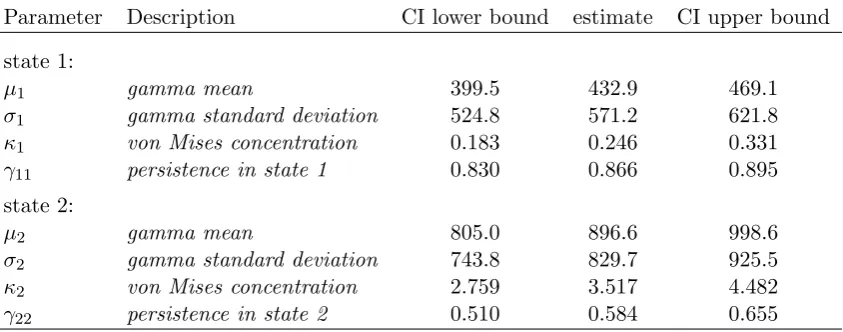
Table 1: Parameter estimates for the group dynamic individual-level model, fitted to the reindeer data, and 95% confidence intervals of the estimates (obtained based on the Hessian of the log-likelihood).

Parameter Description CI lower bound estimate CI upper bound

state 1:

µ1 gamma mean 399.5 432.9 469.1

σ1 gamma standard deviation 524.8 571.2 621.8

κ1 von Mises concentration 0.183 0.246 0.331

γ11 persistence in state 1 0.830 0.866 0.895

state 2:

µ2 gamma mean 805.0 896.6 998.6

σ2 gamma standard deviation 743.8 829.7 925.5

κ2 von Mises concentration 2.759 3.517 4.482

γ22 persistence in state 2 0.510 0.584 0.655

●●●● ●●●●● ●● ●● ●●●●● ●●●●●●● ●●● ●●●● ●●●● ●● ●● ●●●●●●● ●●●●●●●● ●●●●●● ●●

●●●● ●●● ●● ● ●● ●●●●●●●●● ●● ●● ●●●●●● ●●● ●●●●● ●●

●●●● ●●● ●● ●●● ●●●● ●● ●●● ●●●●● ●●●

●●●●●●● ●●● ●●●●●● ●●●●● ●●● ●● ●●●●●●● ●●●●● ● ●●●● ●●●●

●●●●● ●●●● ●●●● ●● ●●●●● ●●●● ●●●●● ●● ●●● ●●●● ●●●●● ●● ●●

●●●●● ●● ●●● ●● ●●●●● ●●● ●●●● ●●●●● ●● ●● ●●●●●●●●●●● ●●●●●●●●● ●● ●●● ●●● ●●●●●●

●● ●●● ●●●● ●●●●●● ●● ●●● ●● ●●● ●● ●●●● ●●●● ●●●●●●●●●●● ●● ●● ●●●●●●●

●●●●●● ●●●● ●● ● ●● ●● ●●●● ●● ●●● ●●●●●●● ●●●●●●● ●● ●●●●●●●●●●●●● ●●●

●●● ●● ●●●● ●●● ● ●●●●●● ●● ●● ●●● ●●●●●●●●●●●

●●●●● ●●● ●●●●●●● ●●●●●●●●●● ●●●● ●●●●●● ●●● ●● ●● ●●●● ●●●●● ●●●●●●●●●

●●● ●● ●●●●● ●● ●●●●●●●●●● ●●●● ●●●● ●●●●

27/06/2003,18:00h 30/06/2003,18:00h 03/07/2003,18:00h 06/07/2003,18:00h

Figure 2: Reindeer example — Viterbi-decoded state sequences for the 11 different individuals. Each grey horizontal line corresponds to one individual, with black dots indicating when the corresponding individual was estimated to be in state 2 of the fitted model.

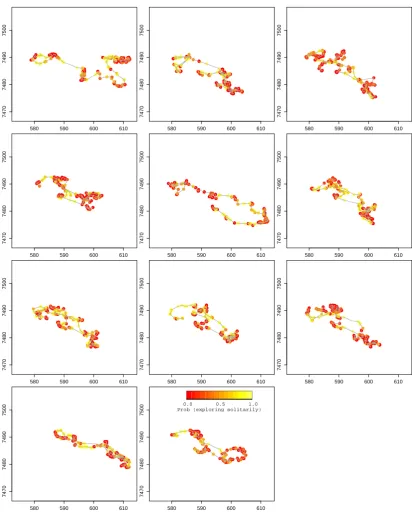
and those steps are slightly biased towards the group centroid (Figure 1). 313 According to the stationary distribution of the fitted Markov chain, approximately three 314 quarters of the time is spent in state 1. Figure 2 displays the Viterbi-decoded state sequences, 315 i.e., the sequences of states that are most likely to have given rise to the observations. Figure 316 3 displays the estimated probabilities of being in the exploratory state (and thus moving in 317 disregard of the group centroid), mapped onto the movement paths, for the 11 reindeer. Broadly 318 speaking, the individual reindeer spend long stretches of time encamped (Figure 2), and these 319 periods are interspersed with brief exploratory forays (shown in yellow in Figure 3). 320

GROUP DYNAMIC MODEL VS. STANDARD MULTI-STATE RANDOM WALK 321

The centroid-driven individual-level model yields a much lower value for the Akaike Information 322 Criterion (AIC) than the simple two-state random walk (∆AIC= 43.6). However, the AIC has 323 to be interpreted very cautiously here: the additional centroid layer appears only in the former 324 model, and the stated ∆AIC is based on regarding the centroid’s positions as deterministic 325 covariates within the individual-level model. In addition to the statistical preference (decreased 326 AIC) for the centroid-driven model, we also illustrate the difference in predictive capacity between 327 the two models using simulation (Figure 4). Although this is a simplified example, it highlights 328 the effect of the group attraction mechanism, which ensures that individuals stick together and 329 follow the group (Figure 4, top row) rather than wander independently and randomly about 330 (Figure 4, bottom row), as is the case for the simple two-state CRW. 331

Discussion

GENERAL REMARKS ABOUT THE APPROACH 333

580 590 600 610 7470 7480 7490 7500 ● ● ● ● ● ●●●●●●●●●●●●●●●●●●●●●●●●●●●●●●●●●●●●●●●● ● ●● ● ● ●●● ● ● ●●●●●●●●● ● ● ● ● ●●●●● ● ●●● ● ● ●●● ● ● ●●●● ● ● ● ● ● ● ● ●●●●●●●● ● ● ● ●●●●● ●● ● ● ● ● ● ●●● ● ●●●● ● ● ● ● ● ● ● ● ● ● ● ● ● ● ● ● ●● ● ● ● ●● ●●●●● ● ●●●●●● ● ● ● ●● ●● ● ● ● ● ● ● ● ● ● ● ● ● ● ● ● ● ● ● ●● ● ● ● ● ●● ● ● ● ● ● ● ● ● ● ● ● ● ●● ●●●●● ●●●●●●●● ● ●

580 590 600 610

7470 7480 7490 7500 ● ● ● ● ● ●●●●●● ● ● ● ●●●●●●●_●● ●● ●●● ●●●●●●●●●●●●●●●●●●●●●●●_●●_●●●●●● ● ● ● ● ● ● ●●●● ● ● ●● ●●● ● ● ● ● ● ● ●●● ● ● ● ●●●● ● ●●● ●●●● ●●●●●●●●●●●●●●●●●●●●●●●●●●●●●●●●●●●●●●●●●●●●●●● ● ● ● ●●_● ● ●_●●●_●●●●●●● ● ●● ● ● ● ● ● ● ● ● ● ● ● ● ● ● ● ● ●●●●●●●●●● ● ● ● ● ●●●●●●●●●●●●●● ● ●●●●●●●● ● ●

580 590 600 610

7470 7480 7490 7500 ● ● ●● ●●●●●●● ● ● ● ● ● ● ●●●●●●●●●●● ● ●●●●●●●●●●● ● ● ● ● ●● ● ●●●● ● ● ● ●●●●●● ● ● ● ● ● ● ●●● ● ● ●●●●● ● ● ● ● ●●●_●●●●●●●●●●●●● ● ●●●● ● ● ● ●●●●●●●●●●●● ●●●●●● ● ● ● ●●●●●●●● ●●●●●●●●● ● ● ● ● ● ● ● ● ● ● ● ● ● ● ● ● ●●●●● ● ●● ● ● ● ● ● ● ● ● ● ● ● ● ●●●●●●●●●●●●●●●●●●●●●● ● ● ● ● ● ● ● ● ● ● ● ●●●● ●●●●●●● ●●

580 590 600 610

7470 7480 7490 7500 ● ● ● ● ● ● ● ● ● ● ● ● ● ● ● ● ● ● ● ● ● ● ●●●●●●●●●●●●●●●●●●● ● ● ● ● ● ●● ● ● ● ● ●●●●●●●●●●●●●● ● ●● ● ●● ● ● ● ● ● ● ● ● ● ● ● ●● ●● ● ● ● ● ●●●●●●●●●● ●●●●●●●●●●●●_{●●●●●} ● ● ● ● ● ● ●●●●●●●●●●● ● ● ● ● ● ● ●● ● ●● ● ● ● ●●● ● ●●●● ● ● ● ● ● ● ● ● ● ● ● ● ● ● ● ● ● ● ● ● ● ● ● ● ● ● ● ● ● ● ● ● ● ●●●●●●●●●●●●●●●● ● ● ● ● ● ● ● ●● ● ● ● ● ● ●● ●

580 590 600 610

7470 7480 7490 7500 ● ● ●● ● ● ● ● ● ●● ● ● ● ● ● ● ● ● ●● ●●● ● ● ● ● ● ●●_●● ● ● ●●● ●●●●●●●●●●●●●●●●●●●●●●●●●●●●●●●●●●●●●●●●●●●●●●●●●●●●●●●●●●●● ● ● ●● ● ● ● ●●● ● ● ● ● ● ●● ● ● ● ● ● ● ● ● ● ●●●●●●● ● ● ● ● ● ● ● ● ● ● ● ● ● ● ● ● ● ●●● ● ● ●●●●●●●● ● ● ● ● ● ● ● ● ● ● ● ● ● ● ● ● ● ● ● ● ● ● ● ● ●●●●●● ●● ● ●●●● ● ● ● ● ●●●●●● ● ● ● ● ● ●●●●●●●●●

580 590 600 610

7470 7480 7490 7500 ● ● ● ● ● ● ● ● ● ● ● ● ●● ● ● ●●●●●●●●●●●●●●●●●● ●●●●●●● ● ● ●●●●● ● ● ● ● ● ● ●●●●●●●●●●● ● ●●● ● ●● ●●●●● ● ● ● ●● ● ● ● ● ●● ● ● ● ●●●●●●●●●●●●●●●●●●●● ● ● ●● ● ● ● ● ● ● ● ● ●_●●●●●●●●●● ●●●●●● ● ● ●●●● ● ● ● ● ● ● ● ● ● ● ●●●●●●●●●● ● ● ● ● ●●● ● ● ● ●●●●●●● ● ● ● ● ● ● ● ● ● ● ● ●● ● ● ● ● ● ● ● ● ● ● ● ● ●● ●● ● ● ●●●●●●● ●

580 590 600 610

7470 7480 7490 7500 ● ● ● ● ● ● ● ● ● ● ● ● ●● ● ● ● ● ● ● ●●● ● ● ● ●●●●●_●●●●● ●●●●● ● ●●●●● ● ● ● ● ● ●●●●●●●●●●●●●●●●●● ● ●●●●● ●●●●●●●●●●●● ● ● ● ● ● ● ●●●●●● ●●●●●●●●●●●●●●●●●●●_●● ● ● ● ● ● ●● ●●●●●●●●●● ● ● ● ● ● ● ● ● ● ● ● ● ●●●●●●●●●●●●●● ● ● ● ● ● ● ● ● ● ● ● ● ● ● ● ● ● ● ● ●●●●_●●● ● ●● ●●●●● ●●●●●●●●●●●●●● ● ● ● ●●●●●●●

580 590 600 610

7470 7480 7490 7500 ●●●●● ● ● ● ● ● ●● ● ● ● ● ● ● ● ● ●●●●●●●●●●●●●●●●● ● ● ● ● ● ● ● ● ● ● ● ● ● ● ● ● ● ●●●●●●●●●●● ●●●● ●●●●●_●●●●●● ●●●_● ●●●●●●●●●●●●●_●●●●●●●●● ● ● ●●●●●●●●●●●●●●●●●●●●●●●●●●●● ●●●● ● ●● ● ●● ● ● ●●●●●●●●●●● ● ●●●●●● ● ● ● ●●●●● ● ● ● ● ● ● ● ● ● ● ● ● ● ● ● ● ● ● ● ● ● ● ● ● ● ● ● ●●●●●● ● ● ● ● ● ● ● ● ● ● ● ●●●●●

580 590 600 610

7470 7480 7490 7500 ● ● ● ● ●●● ● ● ● ● ● ● ● ● ● ● ● ● ● ●●●●_●●●●●●●●●●● ● ●●●●●●●●●● ● ●●●● ● ● ● ●● ● ● ● ●●●●●●●●●● ● ●●●●●_●●●●_●●●●● ● ●●●●● ●●●●●●● ● ● ● ●●●●●●●●●●●_●●●●●●●●●●●●●●●●●●●●●●●●●●●●●●●●●●●● ● ● ●●● ● ●_●●●_●●●●●●● ● ●● ● ● ● ● ● ● ● ● ● ● ● ● ● ● ● ● ● ● ● ● ● ●●●●● ● ● ● ● ● ● ● ● ● ● ● ● ●● ●●●●●●_●● ●●●●●●

580 590 600 610

7470 7480 7490 7500 ● ● ● ● ●● ● ● ● ● ● ● ● ● ● ● ● ● ● ● ● ● ●●● ● ● ● ●●●●●●●●●●● ● ● ● ● ●●●●●●●●●●●●●●●●●●●●●● ● ●●● ●●●●●●●●●●●●●●●_{● ●} ● ●●●●●● ● ● ● ● ● ● ● ● ●● ● ● ● ● ● ● ● ● ● ● ● ● ● ● ●●●●●●●●●●●●●●●● ● ● ● ● ● ● ● ●● ●●● ● ●●●●●●●●●●●● ● ● ●●_●●●●●● ●●●●●●_● ●●●● ● ●●●●●●●● ● ● ● ● ● ● ● ● ● ● ●●●●●●●● ● ● ●_●● ● ● ● ● ● ●● ●

580 590 600 610

7470 7480 7490 7500 ● ●●●●●●● ● ● ● ● ● ● ● ● ● ● ● ● ●●●●●_●●●●●●●●● ● ● ● ●●●● ● ● ● ● ●●_● ● ● ● ● ● ●●●_●● ● ●● ● ● ●●●●●●●●●●●●●●●●●●●●● ● ● ●●●●●●● ● ● ● ●●●●● ●●●●●●●●●●●●●_● ● ● ● ● ● ● ● ● ●● ● ● ● ●●● ●●●●● ● ● ●●●● ● ● ● ● ●●● ● ● ●● ● ● ●●●●●●●●● ●●●● ● ● ● ● ● ● ● ● ● ● ● ● ● ● ● ● ● ● ● ● ● ●●●●●●● ● ●●●●●●●●● ● ●● ● ● ● ● ● ● ●●●●●●●●

0.0 0.5 1.0

Prob (exploring solitarily)

Figure 3: Reindeer example — state categorizations mapped onto the 11 movement paths. The

colour of the points mapped on the locations indicate the probability of the corresponding an-imal being in state 2 (“exploring”), i.e., red indicates higher probability of being encamped and attracted to the group centroid. The horizontal and vertical axes give x and y, respectively, in kilometres using the Sweref99 projection from the National Land Survey of Sweden.

2005), here we fit our model to actual movement data. Furthermore, we are able to statistically 345 compare the fit of competing models (model selection) and to assess the goodness of fit of our 346

model (model checking). 347

Figure 4: Reindeer example — spatial densities of simulated locations of individuals after 9.4 days (left column), 50 days (middle column) and 200 days (right column), for the group dynamic model (top row; with artificial centroid movement straight northwards) and for the standard two-component mixture of correlated random walks (bottom row). The smoothed densities were obtained by applying a bivariate kernel density estimator to the generated locations. Within a short time span (left column) the two models provide similar predictions both in terms of mean and variance of the densities. For simulation over longer time periods (middle and right column), the attraction mechanism in the group dynamic model (top row) both bounds the extreme movements of the individuals (variance) and ensures that individuals follow the group centroid (mean), while the two-state model without attraction (bottom row) is purely diffusive.

state, where individuals are biased toward the group centre, and one or more “exploratory” states 350 where individual movement is independent of the group. In contrast to multi-state CRWs, the 351 fitted group dynamic movement model is non-diffusive. More precisely, even when the attraction 352 to the centroid is weak, individuals will, in the long run, not move arbitrarily far away neither 353

from the centroid nor from each other (cf. Figure 4). 354

One pre-existing approach that is similar in spirit to ours is that of Dunn and Gipson (1977), 355 who formulate all of their models in terms of multiple interacting animals. They think of the 356 position ofm animals inddimensions (takingd= 2 in practice, as we do here) as a single point 357 ink=m×ddimensions, and model the movement of that point using a multivariate Ornstein- 358 Uhlenbeck process, parameterised in terms of a k-vector and two k×k matrices. By contrast, 359 our approach can be thought of as modelling the position of the group in terms of a point and 360 having individuals interact directly with the centroid. Their models have very large numbers 361 of parameters already for moderate values of m, and in practice our representation is far more 362

parsimonious and interpretable, certainly form >2. 363

mechanism of the herding behaviour and therefore has a more intuitive biological interpretation. 370 Using multiple yet relatively short real data time series, we were able to reveal an attraction 371 to the centroid. However, it is difficult to make general statements about how many individuals 372 need to be tracked, or for how long, to make realiable inference on attraction to the centroid. It 373 is also unclear as to how influential the proportion of tracked animals to untracked animals needs 374 to be in terms of reliably estimating the centroid position, but it is intuitive that the model will 375 work best for relatively cohesive groups, where the choice of particular individuals does not bias 376 the analysis. The feasibility of the group centroid concept clearly also depends on the complexity 377 of the fission-fusion dynamics; e.g., the concept of a single group centroid will sometimes be 378

inadequate. 379

DISCUSSION OF RESULTS 380

We generated and analysed simulated data to assess the ability of our modelling approach to 381 consistently estimate model parameters and to distinguish group behaviour from solitary beha- 382 viour in individuals’ movement. When the true location of the group centroid was known, the 383 approach provided unbiased parameter estimates of both the centroid movement model and the 384 individual-level movement model. In cases where the movements of an alpha individual direct 385 the movement of the group, the true centroid location is known when this animal is identified 386 and tagged. This is harder for other species where individual roles in the group are less clear 387 prior to tagging. For scenarios in which the centroid location is unknown, we considered simple 388 or robust means of the individuals’ locations as approximations to the centroid’s locations. In 389 our simulations, the estimation of the individual-level movement models worked reasonably well 390 when the centroid’s locations were approximated using the simple mean, and slightly better when 391 using the robust mean. In addition, we were able to use the centroid attraction information to 392 estimate behavioural states with high accuracy. Our model thus represents a useful approach to 393 statistical and ecological inference on group movement dynamics. 394 We illustrated the modelling approach using movement data from 11 reindeer in Sweden 395 (Skarin et al., 2008, 2010). We were able to infer, to some extent, when individuals are tracking 396 group movement, and when they appear to be following their own movement drivers (cf. Figure 1). 397 The models we fitted to the reindeer data led to the classification that is characteristic of two-state 398 random walks, with an encamped and an exploratory state and corresponding state-dependent 399 step lengths and turning angle distributions (Morales et al., 2004; Langrock et al., 2012), except 400 that in the group dynamic model the encamped state involves the additional feature of a weak 401 attraction to the group centroid. According to the fitted model and based on Viterbi-decoding of 402 the underlying state sequences, some individuals spent periods of up to three days in the nominal 403 encamped state during the time period covered by the observations. 404 Taken together with the simulation results, fitting our model to real data highlights the 405 ecological inference that can be gleaned from our approach. First, we have quantified how the 406 individual reindeer respond to the group. This highlights how conspecific attraction can be 407 included in movement models. Second, we have shown how behavioural states can be estimated 408 with high accuracy, even in cases where important movement phenomena, i.e., step lengths, are 409 similar across states. Finally, we have outlined advantages of including the centroid information 410 over simple multi-state random walks. Specifically, including the centroid layer in the model has 411 led to a more accurate depiction of spatial density, highlighting the importance of incorporating 412

social drivers. 413

EXTENSIONS 414

system and might therefore have reduced bias, but it requires knowledge about which individuals 418 exhibit group behaviour at a given time. Another alternative could be to use a suitable function 419 of the individuals’ locations and movement as a noisy proxy for the location of the centroid. 420 Combining this with a movement model, the location of the centroid could be estimated within 421 a state-space modelling framework, e.g., using a Bayesian data augmentation approach for the 422 centroid location. Such an approach is appealing since the uncertainty about the centroid’s loc- 423 ation would be propagated through to the individual-level parameter estimates, thus potentially 424 providing more accurate parameter estimates and confidence bounds. 425 A simplifying assumption of our method was that all individuals shared movement parameters. 426 A more realistic model could include random effects for certain parameters such as the switching 427 probabilities, thereby allowing for variations in behaviour between individuals (Ford et al., 2012; 428 Schliehe-Diecks et al., 2012), i.e., that some individuals are more adventurous than others. Ran- 429 dom effects, however, describe individual differences as stochasticity (or noise) and hence do not 430 explain the source of the variation. Instead, formulating individual-level parameters as functions 431 of auxiliary information such as, e.g., gender, weight or height, would enable testing of hypotheses 432 related to individual covariates and aid in uncovering reasons for differences between individuals 433

within the group. 434

Similarly, the model can easily be extended to include internal and external dynamic cov- 435 ariates. For example, nonhomogeneous Markov chains could be considered for the behavioural 436 state dynamics, with transition probabilities structured such that observations of the ambient 437 environment or body condition mediate switches between movement phases. Such a model may 438 enable separation of the relative roles of group membership, individual body condition and hab- 439 itat, and represents an exciting avenue of analysis for the movement patterns of social animals. 440 An important special case of such nonhomogeneous Markov chains results from including time 441 as a covariate, which can be useful in order to accommodate seasonality or the daily cycle in the 442 model. Another potentially interesting covariate to consider is the individual-specific separation 443 distance from the centroid, which could be informative about group membership. From the stat- 444 istical point of view, these extension are fairly straightforward, since the likelihood structure of 445

the HMM remains unaffected. 446

Another direction of development is to extend the continuous-time models of Dunn and Gipson 447 (1977) to incorporate some of the advantages of the current approach. Explicitly representing the 448 centroid as part of the process means that the movement of the whole system is then a diffusion 449 process in (m+ 1)×ddimensions, but the modelling of that process is greatly simplified if the 450

m individual animals are each interacting with the centroid, as here, rather than interacting 451 directly with each other. One possibility currently being pursued is for each animal to follow 452 a multivariate Ornstein-Uhlenbeck (MOU) process attracted to the centroid, while the centroid 453 follows its own movement model. Under simplifying assumptions, the whole system can then be 454 modelled as a partially observed (m+ 1)×d-dimensional MOU process. 455

Acknowledgements

References

Blackwell, P.G. (2003) Bayesian inference for Markov processes with diffusion and discrete com- 464

ponents. Biometrika,90, 613–627. 465

Bowler, D.E. & Benton, T.G.. (2005) Causes and consequences of animal dispersal strategies: 466 relating individual behaviour to spatial dynamics. Biological Reviews,80, 205–225. 467

Buhl, J., Sumpter, D.J.T., Couzin, I.D., Hale, J.J., Despland, E., Miller, E.R. & Simpson, S.J. 468 (2006) From disorder to order in marching locusts.Science,312, 1402–1406. 469

Conradt, L., Krause, J., Couzin, I.D. & Roper, T.J. (2009) “Leading according to need” in 470 self-organizing groups. American Naturalist,173, 304–312. 471

Codling, E.A., Plank, M.J. & Benhamou, S. (2008) Random walk models in biology. Journal of 472

the Royal Society Interface,5, 813–834. 473

Couzin, I.D., Krause, J., Franks, N.R. & Levin, S.A. (2005) Effective leadership and decision- 474 making in animal groups on the move.Nature,433, 513–516. 475

Couzin, I.D., Ioannou, C.C., Demirel, G.v., Gross, T., Torney, C.J., Hartnett, A., Conradt, L., 476 Levin, S.A. & Leonard, N.E. (2011) Uninformed Individuals Promote Democratic Consensus 477

in Animal Groups. Science,334, 1578–1580. 478

Croft, D.P., James, R. & Krause, J. (2010)Exploring animal social networks, Princeton University 479

Press. 480

Dowd, M. & Joy, R. (2011) Estimating behavioral parameters in animal movement models using 481

a state-augmented particle filter. Ecology,92, 568–575. 482

Dunn, J.E. & Gipson, P.S. (1977) Analysis of radio telemetry data in studies of home range. 483

Biometrics,33, 85–101. 484

Eftimie, R., de Vries, G., Lewis, M.A. & Lutscher, F. (2007) Modeling group formation and 485 activity patterns in self-organizing collectives of individuals. Bulletin of Mathematical Biology, 486

69, 1537–1565. 487

Ford, J.H., Bravington, M.V. & Robbins, J. (2012) Incorporating individual variability into mark- 488 recapture models. Methods in Ecology and Evolution,3, 1047–1054. 489

Haydon, D.T., Morales, J.M., Yott, A., Jenkins, D.A., Rosatte, R. & Fryxell, J.M. (2008) Socially 490 informed random walks: incorporating group dynamics into models of population spread and 491 growth. Proceedings of the Royal Society B (Biological Sciences),275, 1101–1109. 492

Jonsen, I.D., Flemming, J.M. & Myers, R.A. (2005) Robust state-space modeling of animal 493

movement data.Ecology,86, 2874–2880. 494

Jonsen, I.D., Myers, R.A. & James, M.C. (2006) Robust hierarchical state-space models reveal 495 diel variation in travel rates of migrating leatherback turtles. Journal of Animal Ecology, 75, 496

1046–1057. 497

Langrock, R., King, R., Matthiopoulos, J., Thomas, L., Fortin, D. & Morales, J.M. (2012) Flex- 498 ible and practical modeling of animal telemetry data: hidden Markov models and extensions. 499

Ecology,93, 2336–2342. 500

Mann, R.P. (2011) Bayesian inference for identifying interaction rules in moving animal groups. 501

Morales, J.M., Haydon, D.T., Frair, J.L., Holsinger, K.E. & Fryxell, J.M. (2004) Extracting more 503 out of relocation data: building movement models as mixtures of random walks. Ecology, 85, 504

2436–2445. 505

Morales, J.M., Moorcroft, P.R., Matthiopoulos, J., Frair, J.L., Kie, J.G., Powell, R.A., Merrill, 506 E.H. & Haydon, D.T. (2010) Building the bridge between animal movement and population 507 dynamics. Philosophical Transactions of the Royal Society B,365, 2289–2301. 508

Nagy, M., Akos, Z., Biro, D. & Vicsek, T. (2012) Hierarchical group dynamics in pigeon flocks. 509

Nature,464, 890–899. 510

Nathan, R., Getz, W.M., Revilla, E., Holyoak, M., Kadmon, R., Saltz, D. & Smouse, P.E. (2008) 511 A movement ecology paradigm for unifying organismal movement research. Proceedings of the 512

National Academy of Sciences,105, 19052–19059. 513

Patterson, T.A., Thomas, L., Wilcox, C., Ovaskainen, O. & Matthiopoulos, J. (2008) State-space 514 models of individual animal movement. Trends in Ecology and Evolution,23, 87–94. 515

Patterson, T.A., Basson, M., Bravington, M.V. & Gunn, J.S. (2009) Classifying movement beha- 516 viour in relation to environmental conditions using hidden Markov models. Journal of Animal 517

Ecology,78, 1113–1123. 518

Polansky, L., Wittemyer, G., Cross, P.C., Tambling, C.J. & Getz, W.M. (2010) From moonlight 519 to movement and synchronized randomness: Fourier and wavelet analyses of animal location 520

time series data.Ecology,91, 1506-1518. 521

Polansky, L. & Wittemyer, G. (2011) A framework for understanding the architecture of collective 522 movements using pairwise analyses of animal movement data. Journal of the Royal Society 523

Interface,8, 322-333. 524

Preisler, H.K., Ager, A.A., Johnson, B.K. & Kie, J.G. (2004) Modeling animal movements using 525 stochastic differential equations. Environmetrics,15, 643–657. 526

Schick, R.S., Loarie, S.R., Colchero, F., Best, B.D., Boustany, A., Conde, D.A., Halpin, P.N., 527 Joppa, L.N., McClellan, C.M. & Clark, J.S. (2008) Understanding movement data and move- 528 ment processes: current and emerging directions. Ecology Letters,11, 1338–1350. 529

Schliehe-Diecks, S., Kappeler, P.M. & Langrock, R. (2012). On the application of mixed hidden 530 Markov models to multiple behavioural time series. Interface Focus,2, 180–189. 531

Strombom, D. (2011) Collective motion from local attraction. Journal of Theoretical Biology, 532

283, 145–151. 533

Skarin, A., Danell, ¨O., Bergstr¨om, R. & Moen, J. (2008) Summer habitat preferences of GPS- 534 collared reindeer Rangifer tarandus tarandus.Wildlife Biology,14, 1–15. 535

Skarin, A., Danell, ¨O., Bergstr¨om, R. & Moen, J. (2010) Reindeer movement patterns in alpine 536

summer ranges. Polar Biology,33, 1263–1275. 537

Zucchini, W. & MacDonald, I.L. (2009).Hidden Markov Models for Time Series: An Introduction 538

Appendix S1

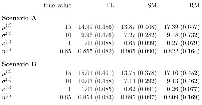
Table S1: Simulation results – means and standard deviations (in brackets) of parameter estim-ates for centroid movement model, as obtained in 500 simulation runs, for centroid approximation methods TL (true location), SM (simple mean) and RM (robust mean). The considered movement model is a (single-state) BCRW, with step length mean parameterµ(c), step length standard de-viation parameter σ(c), directional distribution concentration parameterκ(c), and η(c) the weight of the CRW component in the BCRW (such that 1−η(c) is the weight of the BRW component; see Langrocket al., 2012).

true value TL SM RM

Scenario A

µ(c) 15 14.99 (0.486) 13.87 (0.408) 17.39 (0.657)

σ(c) 10 9.96 (0.476) 7.27 (0.282) 9.48 (0.732)

κ(c) 1 1.01 (0.088) 0.65 (0.099) 0.27 (0.079)

η(c) 0.85 0.855 (0.082) 0.905 (0.090) 0.822 (0.164)

Scenario B

µ(c) 15 15.01 (0.491) 13.75 (0.378) 17.10 (0.452)

σ(c) 10 10.03 (0.458) 7.13 (0.292) 9.13 (0.462)

κ(c) 1 1.01 (0.085) 0.62 (0.091) 0.26 (0.077)

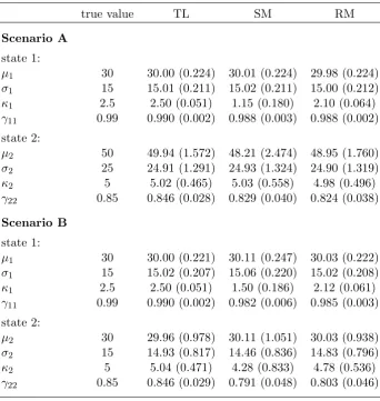
Table S2: Simulation results – means and standard deviations (in brackets) of parameter es-timates for individual-level movement model, as obtained in 500 simulation runs, for centroid approximation methods TL (true location), SM (simple mean) and RM (robust mean). The considered movement model is a two-state HMM (see main manuscript for details).

true value TL SM RM

Scenario A

state 1:

µ1 30 30.00 (0.224) 30.01 (0.224) 29.98 (0.224) σ1 15 15.01 (0.211) 15.02 (0.211) 15.00 (0.212)

κ1 2.5 2.50 (0.051) 1.15 (0.180) 2.10 (0.064)

γ11 0.99 0.990 (0.002) 0.988 (0.003) 0.988 (0.002)

state 2:

µ2 50 49.94 (1.572) 48.21 (2.474) 48.95 (1.760) σ2 25 24.91 (1.291) 24.93 (1.324) 24.90 (1.319)

κ2 5 5.02 (0.465) 5.03 (0.558) 4.98 (0.496) γ22 0.85 0.846 (0.028) 0.829 (0.040) 0.824 (0.038)

Scenario B

state 1:

µ1 30 30.00 (0.221) 30.11 (0.247) 30.03 (0.222)

σ1 15 15.02 (0.207) 15.06 (0.220) 15.02 (0.208) κ1 2.5 2.50 (0.051) 1.50 (0.186) 2.12 (0.061)

γ11 0.99 0.990 (0.002) 0.982 (0.006) 0.985 (0.003)

state 2:

µ2 30 29.96 (0.978) 30.11 (1.051) 30.03 (0.938) σ2 15 14.93 (0.817) 14.46 (0.836) 14.83 (0.796)

κ2 5 5.04 (0.471) 4.28 (0.833) 4.78 (0.536)

γ22 0.85 0.846 (0.029) 0.791 (0.048) 0.803 (0.046)

Table S3: Simulation results – mean proportions of the individual’s states that were correctly decoded by the Viterbi algorithm, which was applied in each of 500 simulation runs, based on models fitted using the centroid approximation methods TL (true location), SM (simple mean) and RM (robust mean), respectively.

TL SM RM

Scenario A 99.4% 98.8% 99.1%