On the Maximum Displacement and Static Buckling of a Circular Cylindrical Shell

(1)

https://www.scirp.org/journal/jamp ISSN Online: 2327-4379

ISSN Print: 2327-4352

DOI: 10.4236/jamp.2019.711196 Nov. 21, 2019 2868 Journal of Applied Mathematics and Physics

On the Maximum Displacement and Static

Buckling of a Circular Cylindrical Shell

G. E. Ozoigbo

1*

, A. M. Ette

2

1_{Department of Mathematics/Computer Science/Statistics & Informatics, Alex Ekwueme Federal University}_{Ndufu-Alike, Ikwo,}

Ebonyi State, Nigeria

2_{Department of Mathematics, Federal University of Technology, Owerri, Imo State, Nigeria}

Abstract

The static buckling load of an imperfect circular cylindrical shell is here de-termined asymptotically with the assumption that the normal displacement can be expanded in a double Fourier series. The buckling modes considered are the ones that are partly in the shape of imperfection, and partly in the shape of some higher buckling mode. Simply-supported boundary conditions are considered and the maximum displacement and the static buckling load are evaluated nontrivially. The results show, among other things, that gener-ally the static buckling load,

λ

S decreases with increased imperfection and

that the displacement in the shape of imperfection gives rise to the least static buckling load.

Keywords

Static, Maximum Displacement, Circular, Cylindrical Shell

1. Introduction

Cylindrical shells have wide engineering applications such as in the construction and study of aircraft, spacecraft and nuclear reactor, tanks for liquid and gas storage and pressure vessels, etc. The analyses of the buckling of cylindrical shells under various loading conditions have been made in the past years and both theoretical and experimental studies have been considered just as in [1] and [2]. Earlier studies on the buckling of shells were done by [3] [4] [5] [6] and [7], while Amazigo and Frazer [8], studied the buckling under external pressure of cylindrical shells with dimple-shaped initial imperfection. It would be recalled that Budiansky and Amazigo [9], investigated the buckling of infinitely long im-perfect cylindrical shells subjected to static loads and Ette and Onwuchekwa [10],

How to cite this paper: Ozoigbo, G.E. and Ette, A.M. (2019) On the Maximum Dis-placement and Static Buckling of a Circular Cylindrical Shell. Journal of Applied Ma-thematics and Physics, 7, 2868-2882.

https://doi.org/10.4236/jamp.2019.711196

Received: August 18, 2019 Accepted: November 18, 2019 Published: November 21, 2019

http://creativecommons.org/licenses/by/4.0/

(2)

DOI: 10.4236/jamp.2019.711196 2869 Journal of Applied Mathematics and Physics

equally studied the static buckling of an externally pressurized finite circular cy-lindrical shell using asymptotic method. In this regard, mention must be made of Lockhart and Amazigo [11], who used perturbation method to investigate the dynamic buckling of finite circular cylindrical shells with small arbitrary geome-tric imperfections under external step-loading. In the same way, Bich et al. [12], by using analytical approach, investigated the nonlinear static and dynamic buck-ling behaviour of eccentrically shallow shells and circular cylindrical shells based on Donnell shell theory. Relevant studies on the buckling analysis were investi-gated in [13] [14] [15] and [16] and Ette [17] [18] [19] [20] and [21].

In this study, we consider a statically loaded imperfect finite circular cylin-drical shell and aim at determining the maximum displacement and the static buckling load for the case where the displacement is partly in the shape of im-perfection and partly in some other buckling mode. The analysis is purely on the use of asymptotic expansions and perturbation procedures.

This analysis is organised as follows. We shall first write down the governing equations as in Amazigo and Frazer [8] and Budiansky and Amazigo [9]. Using the techniques of regular perturbation and asymptotics, we shall analytically termine a uniformly valid expression of the displacement which is followed de-termining by the maximum displacement. Lastly, we shall reverse the series of maximum displacement and determine the static buckling load.

2. Formulation

As in [11], the general Karman-Donnell equation of motion and the compatibil-ity equation governing the normal deflection W X Y

(

,

)

and Airy stress

func-tion F X Y

(

,

)

for cylindrical shell, of length L, radius R, thickness h, bending

stiffness

₍

3 2

₎

12 1 Eh D

υ

=

− (where E and

υ

are the Young’s modulus and Poisson’s

ratio respectively), mass per unit area

ρ

, subjected to external pressure per unit area P, are

4

,

1 1 1

, 2

XX

F W S W W W

Eh R

 

∇ − = − _ + _

  (2.1)

(

)

(

)

(

)

4

, _, _,

1 1

, 2

XX _XX _YY

D W F P W W W W S W W F

R α

 

∇ + + _ + + + _= +

  (2.2)

,XX ,XX 0 at 0, , 0 , 0 2 .

W =W = =F F = X = L <X < π < < πY (2.3)

where, X and Y are the axial and circumferential coordinates respectively and

(

,

)

W X Y , is a continuously differentiable stress-free and time independent

im-perfection. In this work, an alphabetic subscript placed after a comma indicates partial differentiation while S is the symmetric bi-linear operator in X and Y

given by

(

,

)

,XX ,YY ,YY ,XX 2 ,XY ,XY

S P Q =P Q +P Q − P Q (2.4a)

(3)

DOI: 10.4236/jamp.2019.711196 2870 Journal of Applied Mathematics and Physics 2

2 2

4

2 2

X Y

 ∂ ∂ 

∇ =_ + _

∂ ∂

  (2.4b)

here, we shall neglect both axial and circumferential inertia and shall similarly assume simply-supported boundary conditions and neglect boundary layer effect by assuming that the pre-buckling deflection is constant.

As in [11] and [22], we now introduce the following non-dimensional quanti-ties.

2 2

2 2 2

, , , ,

X h W L RP L

x H w

L R ε h λ D ξ R

π

= = = = =

π π (2.5a)

( )

(

)

(

)

2 2

2

2 2

12 1

, , ,

1

L

Y W A

y w K A

R h Rh

υ ξ

ξ

−

= = = − =

π

+ (2.5b)

where,

υ

is Poisson’s ratio and

ε

is a small parameter which measures the amplitude of the imperfection while L is the length of the cylindrical shell which is simply-supported at x= π0, .

We shall neglect boundary layer effect by assuming that the pre-buckling def-lection is constant so that we let

(

)

2 2

1 1

2 2 1

Eh L

F PR X Y f

R

α

ξ

 

 _{ } _

= − _ + _{ }+



  _π + _ (2.7a)

2 1

1 2 PR

W hw

Eh

αυ

 ₋ 

 

 

= + _(2.7b)

where, P is the applied static load and

λ

_{is the non-dimensional load}

ampli-tude. The first terms on the right hand sides of (2.7a) and (2.7b), are pre-buckling approximations, while the parameter

α

, shall take the value

α

=1, if pressure

contributes to axial stress through the ends, otherwise

α

=0, if pressure only

acts laterally.

Substituting (2.7a) and (2.7b) into (2.1 and (2.2), using (2.5a) and (2.5b), and simplifying results to

(

)

2

(

)

2

4

,

1

1 1 ,

2

xx

f ξ w H ξ s w w εw

∇ − + = − + _ + _

  (2.8)

and

( )

(

)

(

)

( ) (

)

4

, , ,

1

, 2

xx xx yy

w K ξ f λ α w εw w εw  HK ξ s w εw f

∇ − + _ + + + _= − +

  (2.9)

,xx ,xx 0 at 0, , 0 , 0 2 , 0 1,

w=w = =f f = x= π < < πx < < πy <ε (2.10)

where,

(

)

4 2 2 2

, , , , , , 2 2

, xx yy yy xx 2 xy xy,

s P Q P Q P Q P Q

x ξ y

 ∂ ∂ 

= + − ∇ =_ + _

∂ ∂

  (2.11)

3. Classical Buckling Load

(4)

asso-DOI: 10.4236/jamp.2019.711196 2871 Journal of Applied Mathematics and Physics

ciated linear perfect structure and its equations, from (2.8) and (2.9) are

(

)

2

4

,

1 xx 0

f

ξ

w

∇ − + = (3.1)

and

( )

4

, , ,

1

0 2

xx xx yy

w K ξ f λ αw w 

∇ − + _ + _=

  (3.2)

,xx 0, ,xx 0 at 0, .

w=w = f = f = x= π (3.3)

The solution to (3.1)-(3.3) is a superposition of the form

(

w f,

) (

= a_mk,b_mk

) (

sin ky+φ_mk

)

sinmx (3.4)

where,

(

a_mk,b_mk

) ( )

≠ 0, 0 and

φ

mk is an inconsequential phase.

On substituting (3.4) into (3.1), using (3.3) and after lengthy simplification, we get

(

)

(

)

2 2

2

2 2

1 mk

mk

m a b

m k

ξ ξ + = −

+ (3.5)

Substituting (3.5) into (3.2) and simplifying, yields

(

)

( ) (

)

(

)

(

)

(

)

2 4 2

2 2

2

2 2

2

2 4

2

2 2

1

1 1

2

K m

m k

k m m

m k

ξ ξ

ξ

ξ λ

ξ ξ α

ξ

+

+ −

+ =

+ +

+

(3.6)

Thus, if n is the critical value of k that minimizes

λ

, then, the value of

λ

at

k=n was taken as the classical buckling load

λ

_C. Thus, in this case, we get

d 0 dk

λ ₌

(3.7)

Therefore, corresponding to k=n,we see that (3.6) is now equivalent to

(

)

( ) (

)

(

)

(

)

(

)

2 4 2

2 2

2

2 2

2

2 4

2

2 2

1

1 1

2

K m

m n

n m m

m n

ξ ξ

ξ

ξ λ

ξ ξ α

ξ

+

+ −

+ =

+ +

+

(3.8)

Usually, m and n take the values m=1, 2, 3, and n=0,1, 2,

We recall that [23] had assumed that k varies continuously, and so, minimized

λ

_{with respect to}_k_{. If} m=1 is the nontrivial values of m and we let ζ ξ₌ _n2,

then, we have

(

)

(

)

2 2

2 1

1 1 2

C

A

ζ

ζ λ

α ζ

+ +

+ =

+ (3.9)

(5)

(

)

2 1

(

1

)

1

, 1, sin sin

1 n n

w f ξ a ky φ x

ζ _ _ ₊ _ _   = _ −_ _ _ + + _   _

  (3.10)

4. Static Theory

In this section, we shall derive the equations satisfied by the displacement and Airy stress functions when the static load is applied.

Similar to (2.8) and (2.9), the structure satisfies the following equations at static loading

(

)

2

(

)

2

4

,

1

1 1 ,

2

xx

f ξ w H ξ s w w εw

∇ − + = − + _ + _

  (4.1)

and

( )

(

)

(

)

( ) (

)

4 , , , 1 , 2

xx xx yy

w K ξ f λ α w εw ξ w εw  HK ξ s w εw f

∇ − + _ + + + _= − +

  (4.2)

,xx ,xx 0 at 0,

w=w = =f f = x= π (4.3)

We now assume the following asymptotic expansions

( ) ( ) 1 i i i i w w

f _f ε

∞ =     =     _ _

 

∑

_ _ (4.4)

Substituting (4.4) into (4.1) and (4.2), and equating the coefficients of orders of i, 1, 2, 3,

i

ε = , the following equations are obtained

( )

₍

₎

( ) ( )

_{( )}

( )

(

( )

)

(

( )

)

2 1 1 4 ,

1 1 1 1

4 , , , 1 0. : ₁ 0 2 xx xx xx yy f w

w K f w w w w

ξ

ε

ξ

λ

α

ξ

∇ − + =   _ _ ∇ − + + + + =  _ _   

 (4.5)

( )

₍

₎

( )

₍

₎

(

( ) ( )

)

(

( )

)

( )

_{( )}

( ) ( ) ( )

( )

(

( ) ( )

)

(

( )

)

2 2

2 2 1 1 1

4

,

2 2 2 2

2 4

, , ,

1 1 1

1

1 1 , ,

2 1 : 2 , , xx

xx xx yy

f w H s w w s w w

w K f w w

HK s w f s w w

ξ ξ

ε ξ λ α ξ

ξ _∇ _{− +} _{= −} ₊  ₊   _ _   _ _ ∇ − + +  _ _     _{= −} _ ₊ _  _ _   (4.6)

( )

₍

₎

( )

₍

₎

(

( ) ( )

)

(

( )

)

( )

_{( )}

( ) ( ) ( )

( )

(

( ) ( )

)

(

( ) ( )

)

(

( )

)

2 2

3 3 1 2 2

4

,

3 3 3 3

3 4

, , ,

1 2 2 1 2

1 1 , ,

1 :

2

, , ,

xx

xx xx yy

f w H s w w s w w

w K f w w

HK s w f s w f s w f

ξ ξ

ε ξ λ α ξ

ξ _∇ _{− +} _{= −} ₊  ₊     _∇ ₋ ₊  ₊   _ _     _{= −} _ ₊ ₊ _  _ _ 

 (4.7)

etc.

We seek solutions to (4.5)-(4.7) in the form

( ) ( ) ₍ _{) (} ₎ ( ) ( ) ( ) ( ) 1 2

1 , 0

1 2

cos sin sin

i i i i i i k p f f f

py py kx

w w w ∞ = =             = +     _    _

(6)

and now assume

(

,

)

sin sin

w x y =a mx ny (4.9)

As earlier obtained, we shall need the following simplifications

2

2 2 4 4 4

4 2

2 2 4 2 2 2 4

x ξ y x ξ x y ξ y

∂ ∂   ∂ ∂ ∂ 

∇ =_ + _ =_ + + _

∂ ∂ ∂ ∂ ∂ ∂

    (4.10a)

so that, if

( ) ( )

1 1 1

cos sin

f = f_Γ py kx

then, we have

( )

(

)

( )

1 2 ₁ 1

4 2 2

1

cos sin , 1, 2

f k ξp f_Γ py kx

∇ = + Γ = (4.10b)

and, if

( ) ( )

2 2 2

sin sin

f = f_Γ py kx

we get

( )

(

)

( )

2 2 ₂ 2

4 2 2

2

sin sin , 1, 2

f k ξp fΓ py kx

∇ = + Γ = (4.10c)

We shall use the fact that

( )

(

)

2

2 1

A K ξ

ξ = −

+ (4.10d)

Solution of Equations of First Order Perturbation The equations necessary here, from (4.5), are

( )1

₍

₎

2 ( )1 4

,

1 _xx 0

f

ξ

w

∇ − + = (4.11)

and

( )1

_{( )}

( )1

(

( )1

)

(

( )1

)

4

,

, ,

1

0 2

xx

xx yy

w K ξ f λ α w w ξ w w 

∇ − + _ + + + _=

  (4.12)

Substituting (4.8) and (4.9) into (4.11), using (4.10a), (4.10b) and (4.10c), multiplying the resultant equation through by cosnysinmx and integrating

with respect to y from 0 to 2π and with respect to x from 0 to π, we note that for

,

p=n k=m, we easily get

( )

(

)

( )

(

)

2 1 2

1 1

1 ₂ ₂ 2

1

m w

f

m n

ξ ξ + = −

+ (4.13)

Similarly, by multiplying the resultant equation through by sinnysinmx, and

integrating with respect to y from 0 to 2π and with respect to x from 0 to π, and for p=n k, =m, we obtain

( )

(

)

( )

(

)

2 1 2

1 2

2 2

1

m w

f

m n

ξ ξ + = −

+ (4.14)

(7)

(4.10b) and (4.10c), thereafter multiplying the resultant equation by sinnysinmx

and integrating with respect to x from 0 to π and y from 0 to 2π, and for

,

p=n k=m, we get

(

₂ ₂

)

2 ₂ ₂ ( )₁

_{( )}

₂ ( )₁ ₂ ₂

2 2

1 1

2 2

m nξ λ αm nξ w K ξ m V λa αm nξ

 ₊ ₋  ₊  ₊ ₌  ₊ 

   

 _ _ _ _

  (4.15)

On substituting for ( )1 2

f from (4.14) and K

( )

ξ from (4.10d) in (4.15) and

simplifying, yields

( )1

2 0

w =B (4.16)

where,

(

)

2 2

0 2

0

2 2 2

2 2 2 2 2

0 2 2

1 2

,

1 2

a m n

B

m A

m n m n

m n

λ α ξ

ϕ

ϕ ξ λ α ξ

ξ

 ₊ 

 

 

=

  _ _

= + +_ _ − _ + _

+  

 

(4.17)

Next, multiplying the resultant equation by cosnycosmx and integrating

with respect to x and y from 0 to π and 0 to 2π, respectively for p=n k, =m,

and simplifying, we get

( )1

1 0

w = (4.18)

We therefore expect from (4.8) that for i=1

( ) ( )

(

)

(

)

2 2

1 1

0 0 0 0 2

2 2

1

sin sin ; sin sin , m

w B mx ny f B mx ny

m n

ξ ξ +

= = −Φ Φ =

+ (4.19)

Solution of Equations of Second Order Perturbation

Equations of the second order to be solved are from (4.6), namely

( )2

₍

₎

2 ( )2

₍

₎

2

(

( )1 ( )1

)

(

( )1

)

4

,

1

1 1 , ,

2

xx

f ξ w H ξ  s w w s w w 

∇ − + = − + _ + _

  (4.20)

and

( )

_{( )}

( ) ( ) ( )

( )

(

( ) ( )

)

(

( )

)

2 2 2 2

4

, , ,

1 1 1

1 2

, ,

xx xx yy

w K f w w

HK s w w s w w

ξ λ α ξ

ξ

 

∇ − + _ + _

 

 

= − _ + _

(4.21)

Evaluating the symmetric bi-linear functions on the right hand sides of (4.20) and (4.21), substituting the same and simplifying, we get (after simplifying tri-gonometric terms)

( )2

₍

₎

2 ( )2

₍

_{) ( )}

2 2

₍

₎

4 2

, 0 0

1

1 1 cos 2 cos 2

2

xx

f ξ w H ξ mn  B B a mx ny 

∇ − + = − + __ + _ + _

 

 (4.22)

and

( )

_{( )}

( ) ( ) ( )

( )( )

(

)

2 2 2 2

4

, , ,

2 2

0 0 0

1 2

cos 2 cos 2

xx xx yy

w K f w w

HK mn B aB mx ny

ξ λ α ξ

ξ

 

∇ − + _ + _

 

 

= − _Φ + _ +

(8)

Next we substitute (4.8) and (4.9) into (4.22), assuming (4.10a), (4.10b) and (4.10c), for i=2. Thereafter, we multiply the resultant equation through by

cos 2nysinmx and integrate with respect to x and y, to get

( ) ( )

(

)

(

)

(

)

(

)

2 2 2

1 1 0 0 2 1

2 2

1 ₂ ₂ 2 2 ₂ ₂ 2

1

, 2

4 1 1

, ,

4 4

f B B a w

Hmn m

m odd

m n m n

ξ ξ

 

= Φ _ + _− Φ

 

+ +

Φ = Φ = =

π + π +

(4.24)

Similarly, we next multiply the resultant equation by sinnysinmx and

inte-grate as usual, and for p=n k, =m, we get

( )

(

)

( )

(

)

2 2 2

2 2

2 ₂ ₂ 2

1

.

m w

f

m n

ξ ξ + = −

+ (4.25)

Next, we substitute (4.8) and (4.9) into (4.23), using (4.10a), (4.10b) and (4.10c), for i=2, and then multiply the resultant equation through by cos 2nysinmx

and integrate, as usual for p=2 ,n k=m to get

( )2

(

2

)

2

1 5 5 3 0 0 0 0 4 0 0

1 ,

2

w = Φ Φ = Φ B Φ + ΦB a + Φ _ B +B a_

  (4.26)

( )

(

)

2

3 ₂ 2

2

2 2 2 2

2 2

( )

1

4 4

2 4

mn HK

m A

m n m n

m n

ξ

λ

α

ξ

Φ =

   

+ +_ _ − _ + _

+  

 

(

) (

)

3 2 2

4 2

2

2 2

2 2 2 2 2 2

2 2

4

1

4 4 4

2 4

m n A

m A

m n m n m n

m n

ξ ξ λ α ξ

ξ Φ =

 _ _ _ _

 

+ + +_ _ − _ + _

+  

   

 

(4.27)

In the same manner, multiply the resultant equation by sinnysinmx and

in-tegrate with respect to x and y, for p=n k, =m, and simplify to get

( )2 ( )2

2 0, 2 0

w = f = (4.28)

Therefore, we observe from (4.8), and for i=2, that

( )2 ( )2 ( )2 ( )2

1 cos 2 sin ; 1 cos 2 sin ,

w =w ny mx f = f ny mx (4.29)

On substitution in (4.29) using (4.24) and in the first part of (4.26), we get

( )2 ( )2

5 10

2

10 1 0 0 2 5

cos 2 sin ; cos 2 sin , 1

2

w ny mx f ny mx

B B a

= Φ = Φ

   

Φ = Φ_ _ + _− Φ Φ _

 

 

(4.30)

Solution of Equations of Third Order Perturbation The actual equations of the third order are from (4.7), namely

( )3

₍

₎

2 ( )3

₍

₎

2

(

( )1 ( )2

)

(

( )2

)

4

,

1 xx 1 , ,

f ξ w H ξ s w w s w w 

∇ − + = − + _ + __(4.31)

(9)

( )

_{( )}

( ) ( ) ( )

( )

(

( ) ( )

)

(

( ) ( )

)

(

( )

)

3 3 3 3

4

, , ,

1 2 2 1 2

1 2

, , ,

xx xx yy

w K f w w

HK s w f s w f s w f

ξ λ α ξ

ξ

 

∇ − + _ + _

 

 

= − _ + + _

(4.32)

Evaluating the symmetric bi-linear functions on the right sides of (4.31) and (4.32) and substituting the same and simplifying, yields

( )

₍

₎

( )

(

) ( ) (

)

[

]

2

3 3

4

,

2 2

5 0 5

1

1 9 sin 3 sin

4

cos 2 sin 3 9 cos 2 sin

xx

f w

H mn B a ny ny

mx ny mx ny

ξ

∇ − +

= − + Φ + Φ −

− +

(4.33)

and

( )

_{( )}

( ) ( ) ( )

( )( )

[

]

3 3 3 3

4

, , ,

2 2

0 5 0 0 1 0 0 2 5

2

1 0 0 2 5

1 2

1 1

4 2

1

9 sin 3 sin

2

cos 2 sin 3 9 cos 2 sin

xx xx yy

w K f w w

HK mn B B B B a

a B B a ny ny

mx ny mx ny

ξ λ α ξ

ξ

 

∇ − + _ + _

 

    

= − −Φ Φ + Φ _ + _− Φ Φ 

 





   

+ _Φ _ + _− Φ Φ _ −

 

 

− +

(4.34)

We observe from the simplifications on the right hand sides of (4.33) and (4.34) that there will be four buckling modes generated wi r p( )(3, ) with their

re-spective Airy stress functions ₍( )3 ₎ , i r p

f . These buckling modes correspond to the

following terms on the right hand sides of (4.33) and (4.34) : sin 3nysinmx, sinnysinmx, cos 2mxsin 3ny and cos 2mxsinny.

However, of the four modes, it is only the mode in the shape of sinnysinmx

that is in the shape of the imperfection. We shall consider this mode and the ad-ditional mode in the shape of sin 3nysinmx.

We now substitute (4.8) and (4.9) into (4.33), using (4.10a), (4.10b) and (4.10c), for i=3, and thereafter, multiply the resultant equation through by sin 3nysinmx

and integrate and for k=m, p=3n, to get

( )

(

)

(

)

(

)

( )( )

2 2

3 2 2 3

0

2 ,3 2 2 ,3

2 2

1 9

1 1

9

m n m n

f H mn A m w

m n

ξ ξ

ξ

 

= _ + − + _

π

 

+ (4.35)

In the same way, we multiply the resultant equation by sinmxsinny, integrate

and for k=m, p=n, to get

( )

(

)

(

)

2

(

)

2 ( )( )

3 2 2 3

0

2 , 2 2 ,

2 2

3

0 0 0 0 5 2 3

0 0

1 1

1 1 ,

1 1

,

m n m n

f H mn A m w

m n

A B l l a

B B

ξ ξ

ξ

 

= _π + − + 

 

+

 

= = Φ  + 

 

(4.36)

We next substitute (4.8) and (4.9) into (4.34), using (4.10a), (4.10b) and (4.10c), for i=3. Thereafter, we multiply the resultant equation by sin 3nysinmx,

(10)

( )

(

_{) (}

₎

(

)

( )

3 0 0 1 01

2 ,3 2

2 2

2 2 2 2

2 2

3 2 2 2

0 2 1

2 2

3

01 0 01 01 1 2 0 5 1 2 2 5

0 0 0 , 1 9 9 2 9 9 9 , , 9

1 1 1 1

, 2 m n A A w m A

m n m n

m n

Hm n A HK mn

m n

A B l l a

B

B B

ξ λ α ξ

ξ

ξ ξ

Θ − Θ

=   _ _   + + − _ + _  +     

Θ = Θ =

π

π +

= = Φ − Φ Φ + Φ − Φ Φ

(4.37)

Similarly, we multiply through by sinnysinmx and note that for k=m p, =k,

we get

( )

(

_{) (}

₎

(

)

( )

3 2 01 3 0

2 , 2

2 2

2 2 2 2

2 2

3 2 2 2

3 2 2

2 2 , 1 2 1 1 , m n A A w m A

m n m n

m n

Hm n A HK mn

m n

ξ λ α ξ

ξ

ξ ξ

Θ − Θ

=   _ _   + + − _ + _  +     

Θ = Θ =

π

π +

(4.38)

Thus, of the four non-zero buckling modes of this order and their respective Airy stress function, the ones we shall consider are

( ) ( ) ( ) ( ) ( ) ( ) ( ) ( ) 3 3

2 ,3 2 ,

3 3

2 ,3 2 ,

sin 3 sin , sin sin ,

sin 3 sin and sin sin

m n m n

w ny mx w ny mx

f ny mx f ny mx (4.39)

As a summary so far, we can write the displacement and its respective Airy stress functions as

( ) ( ) ( ) ( ) ( ) ( ) ( ) ( ) ( ) ( ) ( ) ( ) ( ) ( ) ( ) ( ) 1 2

2 , ₂ 1 ,2

1 2

2 , 1 ,2

3 3

2 ,3 2 ,

3

3 3

2 ,3 2 ,

sin sin cos sin

sin sin 3 sin sin

m n m n

m n m n

w w

w

mx ny ny mx

f _f _f

w w

mx ny mx ny

f f ε ε ε       _ _ _ _ = +   _ _ _ _   _ _ _ _           + _ + _+             (4.40)

Equation (4.40) determines the displacement and the corresponding Airy stress functions.

5. Values of Independent Variables at Maximum

Displacement

The analysis henceforth will be concerned with the displacement components that are partly in the shape of the imperfection or partly in the shape of sinmxsin 3ny.

In this respect, we neglect the displacements of order _

( )

ε

2 _{in (4.40) so that}

the displacement becomes

( ) ( ) ( ) ( )

{

( ) ( )

}

( )

1 3 3

2 , 2 ,

3 4

2 ,3

sin sin sin sin

sin sin 3

m n m n

m n

w w mx ny w mx ny

w mx ny

ε ε

ε

= +

+ Ω + (5.1)

where,

(11)

When Ω =0, we get the exact displacement that is purely in the shape of

imperfection, but when Ω =1, we get the resultant displacement incorporating

the modes sinmxsin 3ny and sinmxsinny.

Since the displacement w in (5.1) depends on x and y then, the conditions for maximum displacement are as follows

,x ,y 0

w =w = (5.2)

We now let xa and ya be critical values of x and y respectively at

maxi-mum displacement.

From (5.1), using (5.2), we see that for maximum displacement,

;

2 2

a a

x y

m n

π π

= = _(5.3)

where (5.3) are the least nontrivial values of xa and ya.

6. Maximum Displacement

The maximum displacement is obtained from (5.1) at the critical values of x and

y where w has a maximum value. Hence, the value of w at these values becomes

( )

_{( )}

( )

_{( )}

( )

_{( )}

{

}

1 3 3 3

2 , 2 , 2 ,3

a m n m n m n

w =εw λ +ε w λ − Ωw λ + (6.1)

Meanwhile, (6.1) can be recast as

( )

3 4

1 3

a

w =

ε

c +

ε

c +

ε

(6.2)

where,

( )

_{( )}

( )

_{( )}

( )

_{( )}

1 3 3

1 2m n, , 3 2m n, 2m,3n

c =w λ c =w λ − Ωw λ (6.3)

7. Static Buckling Load

The static buckling load,

λ

S according to [24] [25] and [26], is obtained from

the maximization

d 0 dwa

λ

= _(7.1)

The usual procedure (as in [22] [26] and [27]), is to first reverse the series (6.2) in the form

3

1 a 3 a

d w d w

ε= + +__(7.2)

By substituting (6.1) into (7.2) and equating the coefficients of powers of or-ders of

ε

, we get

3

1 3 4

1 1

1

, c

d d

c c

= = − _(7.3)

The maximization in (7.1) easily follows from (7.2) where wa is now being

substituted for w to yield, after some simplifications,

1

3 2 3 3

c c

ε = _(7.4)

(12)

(

)

( )

3

2 ₂

2 2

2 2 2 2

2 2

0 1 2

3 3 1

2 2

S

m A

m n m n

m n

a m n

ξ λ α ξ

ξ

λ ε α ξ

 _ _ 

 ₊ ₊ ₋  ₊ 

  ₊  _ _

 

 

 

 

= _ + _Ψ

 

(7.5)

This determines the static buckling load

λ

S of the circular cylindrical shell

structure, and the determination is implicit in the load parameter

λ

S,

where,

(

)

(

)

(

)

₍

₎

2 01 3 0

02

0 2 01 3 0 01 2

01 0

2 2 2

0 0 1 01 2 2 2 2 2

02 2 0 2 2

0

1 , ,

1 ,

2 S

l l

Q

l l Q

Q

l l m A

Q m n m n

m n

ϕ

ϕ ξ λ α ξ

ϕ ξ

Θ − Θ

Ω

Ψ = Θ − Θ − =

 

Θ − Θ _    _

= = + +_ _ − _ + _

+  

   

 

(7.6)

8. Results and Discussion

The result (7.5) is asymptotic in nature. The results of the classical buckling load

C

λ

, and that of the cylindrical shell structure are as seen in (3.9), whereas, the corresponding displacement and Airy Stress function of the structure are as in (3.10). Similarly, the static buckling load

λ

S, is as shown in (7.5). A computer

program in MATLAB gives the relationship between the static buckling load

λ

S,

and the imperfection parameter

ε

, at Ω =0 or Ω =1, and where we have

fixed the following as

α

=1, A=0.2, H=0.2, a =0.02,

ξ

=0.8, m=1

and n=1 is as shown in Table 1.

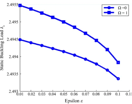
A careful appraisal of the graph of Figure 1, shows that static buckling load

S

λ

, decreases with increased imperfection parameter

ε

. This is expected. In other words, static buckling load

λ

S increases with less imperfection. The value

of static buckling load

λ

S is higher when the buckling mode is a combination

of the modes in the shape of imperfection (sinmxsinny) and shape of other

geometric form (sinmxsin 3ny), i.e. (Ω =1) compared to the case when the

[image:12.595.210.538.555.734.2]

buckling mode is in the shape of imperfection (sinmxsinny) (i.e. Ω =0).

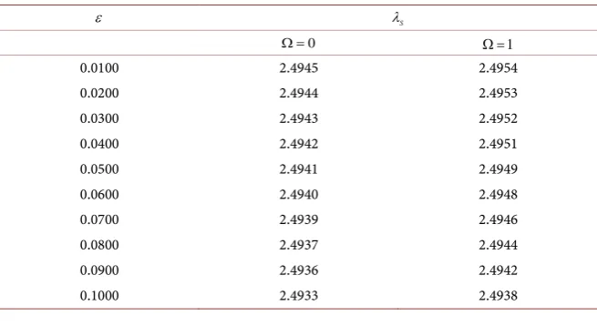
Table 1. Relationship between static buckling load, λS and imperfection parameter, ε

for some values of Ω of the circular cylindrical shell structure using Equation (7.5).

ε λS

0

Ω = Ω =1

0.0100 2.4945 2.4954

0.0200 2.4944 2.4953

0.0300 2.4943 2.4952

0.0400 2.4942 2.4951

0.0500 2.4941 2.4949

0.0600 2.4940 2.4948

0.0700 2.4939 2.4946

0.0800 2.4937 2.4944

0.0900 2.4936 2.4942

(13)

[image:13.595.262.484.69.244.2]

Figure 1. Graph of Static buckling load λS, as a function of imperfection parameter,

ε for some values of Ω of the circular cylindrical shell structure using Table 1.

9. Conclusion

This analysis has analytically determined the maximum of the out-of-plane nor-mal displacement of a finite imperfect cylindrical shell trapped by a static load. We have used the techniques of perturbation and asymptotics to derive an im-plicit formula for determining the static buckling load of the cylindrical shell in-vestigated. The formulation contains a small parameter depicting the amplitude of the imperfection and on which all asymptotic series are expanded. Such an analytical approach can be duplicated for other structures including toroidal shell segments and plates.

Conflicts of Interest

The authors declare no conflicts of interest regarding the publication of this pa-per.

Acknowledgements

This paper is dedicated to the memory of late EZIKE OGBUEHI FELIX IKENNA OZOIGBO, who died on 20th_{day of July, 2019 and to be buried on 22}nd_{day of}

November, 2019.

References

[1] Xu, X.S., Ma, J.Q., Li, C.W. and Chu, H.J. (2009) Dynamic Local and Global Buck-ling of Cylindrical Shells under Axial Impact. Engineering Structures, 31, 1132-1140.

https://doi.org/10.1016/j.engstruct.2009.01.009

[2] Fan, H.G., Chen, Z.P., Feng, W., Fan, Z. and Cao, G.W. (2015) Dynamic Buckling of Cylindrical Shells with Arbitrary Axisymmetric Thickness Variation under Time Dependent External Pressure. International Journal of Structural Stability and Dy-namics, 15, 21 p.https://doi.org/10.1142/S0219455414500539

(14)

[4] Hutchinson, J.W. and Amazigo, J.C. (1967) Imperfect-Sensitivity of Eccentricity Stiffened Cylindrical Shells. AIAA Journal, 5, 392-401.

https://doi.org/10.2514/3.3992

[5] Budiansky, B. and Roth, R.S. (1962) Axisymmetric Dynamic Buckling of Clamped Shallow Spherical Shells. Collected Papers on Stability of Shell Structures, NASA TN D-1510, Washington DC.

[6] Budiansky, B. and Hutchinson, J.W. (1970) Buckling Progress and Challenge in Process of Trends in Solid Mechanics. University Press Delft, Delft, 93-116.

[7] Roth, R. and Klosner, J. (1964) Nonlinear Response of Cylindrical Shells Subjected to Dynamic Axial Loads. AIAA Journal, 2, 1788-1794.

https://doi.org/10.2514/3.2666

[8] Amazigo, J.C. and Frazer, W.B. (1971) Bucklng under External Pressure of Cylin-drical Shells with Dimple-Shaped Initial Imperfection. International Journal of Sol-ids Structures, 7, 883-900.https://doi.org/10.1016/0020-7683(71)90070-9

[9] Budiansky, B. and Amazigo, J.C. (1968) Initial Post-Buckling Behaviour of Cylin-drical Shell under External Pressure. Journal of Mathematical Physics, 47, 233-235.

https://doi.org/10.1002/sapm1968471223

[10] Ette, A.M. and Onwuchekwa, J.U. (2007) On the Static Buckling of an Externally Pressurized Finite Circular Cylindrical Shell. Journal of the Nigerian Association of Mathematical Physics, 11, 323-332.https://doi.org/10.4314/jonamp.v11i1.40226

[11] Lockhart, D. and Amazigo, J.C. (1975) Dynamic Buckling of Externally Pressurized Imperfect Cylindrical Shells. Journal of Applied Mechanics, 42, 316-320.

https://doi.org/10.1115/1.3423574

[12] Bich, D.H., Dung, D.V., Nam, V.H. and Phuong, N.T. (2013) Nonlinear Static and Dynamic Buckling Analysis of Imperfect Eccentrically Stiffened Functionally Graded Circular Cylindrical Thin Shells under Axial Compression. International Journal of Mechanical Science, 74, 190-200.https://doi.org/10.1016/j.ijmecsci.2013.06.002

[13] Paimushin, V.N. (2016) Static and Dynamic Buckling Modes of Spherical Shells Subjected to External Pressure. Russian Mathematics, 60, 37-46.

https://doi.org/10.3103/S1066369X1604006X

[14] Paimushin, V.N. (2017) Static and Dynamic Beam Buckling Shapes of Long Ortho-tropic Cylindrical Shells Undergoing External Pressure. Journal of Applied Mathe-matics and Mechanics, 72, 1014-1027.

[15] Lukankin, S.A. and Paimushin, V.N. (2014) Static and Dynamic Beam Buckling Shapes of Long Orthotropic Cylindrical Shells under External Pressure. Izv. RAS. MTT, No. 1, 108-128.

[16] HuyBich, D., Dung, D.V., Namb, V.H. and Phuong, N.T. (2013) Nonlinear Static and Dynamic Buckling Analysis of Imperfect Eccentrically Stiffened Functionally Graded Circular Cylindrical Thin Shells under Axial Compression. International Journal of Mechanical Sciences, 74, 190-200.

https://doi.org/10.1016/j.ijmecsci.2013.06.002

[17] Ette, A.M. (2003) Buckling of a Cylindrical Shell Pressurized by an Impulse. Journal of the Nigerian Mathematical Society, 22, 82-110.

[18] Ette, A.M. (2004) On the Dynamic Buckling of Stochastically Imperfect Finite Cy-lindrical Shells under Step Loading. Journal of the Nigerian Association of Mathe-matical Physics, 8, 35-46.https://doi.org/10.4314/jonamp.v8i1.39971

(15)

[20] Ette, A.M. (2008) Perturbation Technique on the Dynamic Buckling of a Lightly Damped Cylindrical Shell Axially Stressed by an Impulse. Journal of the Nigerian Association of Mathematical Physics, 12, 103-120.

https://doi.org/10.4314/jonamp.v12i1.45493

[21] Ette, A.M. (2008) Initial Post-Buckling of Toroidial Shell Segments Pressurized by External Load. Journal of the Nigerian Association of Mathematical Physics, 12, 121-132.https://doi.org/10.4314/jonamp.v12i1.45494

[22] Amazigo, J.C. (1974) Asymptotic Analysis of the Buckling of Externally Pressurized Cylinders with Random Imperfections. Quarterly of Applied Mathematics, 32, 429-442.

https://doi.org/10.1090/qam/99693

[23] Batdorf, S.B. (1947) A Simplified Method of Elastic Stability Analysis for Thin Cy-lindrical Shells. NACA Report, 874.

[24] Budiansky, B. (1966) Dynamic Buckling of Elastic Structures, Criteria and Estima-tion. In: Dynamic Stabilities of Structures, Hermann Pergamon, Oxford, 83-106. [25] Hutchinson, J.W. and Budiansky, B. (1966) Dynamic Buckling Estimates. AIAA

Journal, 4, 525-530.https://doi.org/10.2514/3.3468

[26] Amazigo, J.C. and Ette, A.M. (1987) On a Two-Small Parameter Differential Equa-tion with ApplicaEqua-tion to Dynamic Buckling. Journal of Nigerian Mathematical So-ciety, 6, 90-102.

[27] Amazigo, J.C. (1971) Buckling of Stochastically Imperfect Columns on Nonlinear Elastic Foundation. Quarterly of Applied Mathematics, 29, 403-409.