On line scheme for parameter estimation of nonlinear lithium ion battery equivalent circuit models using the simplified refined instrumental variable method for a modified Wiener continuous time model

warwick.ac.uk/lib-publications

Original citation:

Allafi, Walid, Uddin, Kotub, Zhang, Cheng, Mazuir Raja Ahsan Sha, Raja and Marco, James.

(2017) On-line scheme for parameter estimation of nonlinear lithium ion battery equivalent

circuit models using the simplified refined instrumental variable method for a modified

Wiener continuous-time model. Applied Energy, 204 . pp. 497-508.

Permanent WRAP URL:

http://wrap.warwick.ac.uk/90535

Copyright and reuse:

The Warwick Research Archive Portal (WRAP) makes this work of researchers of the

University of Warwick available open access under the following conditions.

This article is made available under the Attribution-NonCommercial-NoDerivatives 4.0 (CC

BY-NC-ND 4.0) license and may be reused according to the conditions of the license. For

more details see:

http://creativecommons.org/licenses/by-nc-nd/4.0/

A note on versions:

The version presented in WRAP is the published version, or, version of record, and may be

cited as it appears here.

On-line scheme for parameter estimation of nonlinear lithium ion

battery equivalent circuit models using the simplified refined

instrumental variable method for a modified Wiener continuous-time

model

Walid Allafi

a,⇑

, Kotub Uddin

a

, Cheng Zhang

a

, Raja Mazuir Raja Ahsan Sha

b

, James Marco

a

a

WMG, The University of Warwick, Coventry CV4 7AL, United Kingdom b

Charge Auto, Oxford Industrial Park, Cassington Road, Yarnton, Oxfordshire OX5 1QU, United Kingdom

h i g h l i g h t s

Off-line estimation approach for continuous-time domain for non-invertible function. Model reformulated to multi-input-single-output; nonlinearity described by sigmoid. Method directly estimates parameters of nonlinear ECM from the measured-data. Iterative on-line technique leads to smoother convergence.

The model is validated off-line and on-line using NCA battery.

a r t i c l e

i n f o

Article history:

Received 31 March 2017

Received in revised form 30 June 2017 Accepted 15 July 2017

Keywords:

Lithium ion battery

Nonlinear equivalent circuit model Online parameter estimation Continuous time wiener model Simplified refined instrumental variable method

a b s t r a c t

The accuracy of identifying the parameters of models describing lithium ion batteries (LIBs) in typical battery management system (BMS) applications is critical to the estimation of key states such as the state of charge (SoC) and state of health (SoH). In applications such as electric vehicles (EVs) where LIBs are subjected to highly demanding cycles of operation and varying environmental conditions leading to non-trivial interactions of ageing stress factors, this identification is more challenging. This paper pro-poses an algorithm that directly estimates the parameters of a nonlinear battery model from measured input and output data in the continuous time-domain. The simplified refined instrumental variable method is extended to estimate the parameters of a Wiener model where there is no requirement for the nonlinear function to be invertible. To account for nonlinear battery dynamics, in this paper, the typ-ical linear equivalent circuit model (ECM) is enhanced by a block-oriented Wiener configuration where the nonlinear memoryless block following the typical ECM is defined to be a sigmoid static nonlinearity. The nonlinear Weiner model is reformulated in the form of a multi-input, single-output linear model. This linear form allows the parameters of the nonlinear model to be estimated using any linear estimator such as the well-established least squares (LS) algorithm. In this paper, the recursive least square (RLS) method is adopted for online parameter estimation. The approach was validated on experimental data measured from an 18650-type Graphite/Lithium-Nickel-Cobalt-Aluminium-Oxide (C6/LiNiCoAlO2) lithium-ion cell. A comparison between the results obtained by the proposed method and by nonpara-metric frequency-based approaches for obtaining the model parameters is presented. It is shown that although both approaches give similar estimates, the advantages of the proposed method are (i) the sim-plicity by which the algorithm can be employed on-line for updating nonlinear equivalent circuit model (NL-ECM) parameters and (ii) the improved convergence efficiency of the on-line estimation.

Ó2017 The Authors. Published by Elsevier Ltd. This is an open access article under the CC BY-NC-ND license (http://creativecommons.org/licenses/by-nc-nd/4.0/).

1. Introduction

Effective real-time control of LIB systems relies on efficient esti-mations of the state of charge (SoC) and state of health (SoH). This

http://dx.doi.org/10.1016/j.apenergy.2017.07.030

0306-2619/Ó2017 The Authors. Published by Elsevier Ltd.

This is an open access article under the CC BY-NC-ND license (http://creativecommons.org/licenses/by-nc-nd/4.0/).

⇑ Corresponding author.

E-mail address:[email protected](W. Allafi).

Contents lists available atScienceDirect

Applied Energy

in turn, depends on operating conditions and usage, particularly the frequency of cycling as well as the complex interactions between voltage, current, temperature and depth of discharge [1–3] during both cycling and storage[4–7]. State estimation is especially important for applications such as electric vehicles (EVs) where the inaccurate estimation of SoC and SoH can lead to over-charge or over-discharge events with significant implica-tions for system safety and reliability[8]. As such, Battery Manage-ment Systems (BMS) typically employ physical models to estimate the states of a given battery through the model parameters[9–13]. To this end, there has been a large body of work focusing on devel-oping methods of estimating LIB model parameters for use within real-time operation. This includes, for example, least square meth-ods[14–18], state observer and adaptive observer techniques[15], [17–19], support vector machines[20]and genetic algorithms[21]. Fleischer et al. [22] summarised the most commonly used methods for on-line estimation LIB model parameters into three subgroups: methods using electrochemical impedance spec-troscopy (EIS), methods employing ECMs and methods based on electrochemical models. EIS methods such as that proposed by Howey et al.[23], [24], where it’s argued that the harmonics gen-erated by the electric motor connected to the EV powertrain can be harnessed to estimate the EIS and hence battery impedance. The challenge in this case, in addition to the requirement for bespoke electronics which may be prohibitively expensive, is the limited range of excitation frequencies present [22]. Furthermore, apart from cell impedance, it is not obvious how EIS can be used to define other important metrics such as the SoC, SoH and cell capac-ity. The second subgroup of parameter estimation methods is based on traditional linear ECMs[22]. To identify the unknown model parameters and states, various implementations of the least squares (LS) method have been applied to estimate the best solu-tion of an overdetermined system which minimises the sum of squared residuals[22]. The variations of LS filters include the RLS filter and the weighted RLS filter [25–32]. Non-recursive filters such as batch learning[33,34], which also employ an iterative LS procedure, enable the estimation of NL-ECM parameters, although this is at a cost of higher memory and computing resource[22]. Furthermore, with such non-recursive filters, high frequency real-time parameters may evolve during the evaluation procedure and therefore may not be up-to-date with the corresponding oper-ating point [22]. More accurate but computationally expensive filters for parameter estimation are based on different implemen-tations of the Kalman filter (KF). The KF is a recursive procedure which combines analytical and probabilistic Bayesian models. Although the assumption of linearity and Gaussian noise in typical KFs are applicable to a wide class of problems, for highly nonlinear model equations such as the case for LIBs, generalisations of the KF are required. Such generalisations include: the dual extended KF [35–37]which consists of two different extended KFs in which the results are calculated in parallel; the joint extended KF [38,39]where model parameters are re-adapted at the same time, thus increasing computing effort due to the higher dimensional

model matrices [22]; the dual sigma-point KF [35]; the joint sigma-point KF[40]; and the particle filter[41]. Although KF based approaches may be more accurate, the computational cost is known to be significantly higher due to the required matrix inver-sions which may lead to numerical instability. To take into consid-eration both the nonlinearity of models and the uncertainties and noise in measurements, nonlinear and robust observers such as H-infinite filters [42,43] and sliding mode observers [44–46]have been applied for battery parameters and state estimation.

Both LS and KF methods have been applied to electrochemistry based battery models[5,47–50]for estimating model parameters. The complex calculations of the models themselves, let alone the adaptive filters, render the applicability of such techniques chal-lenging for many commercial BMS’s that employ low-cost micro-controllers. Furthermore, as discussed in Refs. [5,47], the relatively large number of model parameters associated with elec-trochemical battery models means that parameters are seldom uniquely identifiable. A more detailed review and discussion of commonly used methods for parameter and state estimation are beyond the scope of this work, interested readers are directed to Ref.[22].

Although ECMs are comparatively simple and require less com-putational effort to evaluate[1], [51], they are unable to capture important dynamics such as solid phase diffusion limitation result-ing from large current loads or low ambient temperatures[52]. Electrochemical models on the other hand, which have a recognis-able correspondence with electrochemistry, can readily accommo-date solid phase diffusion [52] – at the expense of extra computational resource, however. The trade-off between model accuracy and computational resource adopted in this work is to consider a Weiner configuration cascade of an ECM coupled with a nonlinear overpotential correction function. The latter is moti-vated by the Butler-Volmer relation and accommodates for the nonlinear voltage response generated by high current densities and/or low temperatures[53]. In the context of real applications, the advantages of the Hammerstein/Wiener/Hammerstein-Wiener class of nonlinear models include: (i) that the dynamics of systems are mainly generated by the linear subsystem so that algorithms and techniques developed for the linear systems may be adopted for the Hammerstein/Wiener model and (ii) if the static nonlinear-ity has an inverse function, such that it allows for a cancellation with the static nonlinearity, then linear control algorithms can be applied. Thus, the adopted Weiner model in this paper can capture the nonlinear dynamics of a LIB while still maintaining a simple model structure with low complexity allowing a suitably simple online estimation technique to be adopted.

The estimation approach of the Wiener models can either be categorised as iterative or non-iterative. This work has primarily focused on iterative methods. In the discrete time-domain, the iter-ative algorithm proposed in[54]is based on accessing the internal signals by using the key term separation principle as a decomposi-tion technique. This algorithm was extended for the case of multi-inputs by Vörös in[55]. The approach adopted in[54,55]express Nomenclature

BMS battery management system ECM equivalent circuit model

EIS electrochemical impedance spectroscopy EV electric vehicle

KF Kalman filter LIB lithium ion battery LS least squares NL-ECM nonlinear ECM

OCV open circuit voltage RC resistor-capacitor RLS recursive least squares SoC state of charge SoH state of health Wm Wiener model

the Hammerstein and Wiener models in a linear-in-the-parameter manner. The key term separation principle and estimated linear outputs, adopted in[54,55], are also used in the case of the Wiener model in [56]. The principle drawbacks of this approach are namely, that it is not a direct identification method and the conver-gence is not guaranteed. Other approaches for discrete iterative methods can be found in [57]. In recent studies in the discrete domain, the kernel, Volterra and fractional least mean square algo-rithms have been applied for estimating the parameters of the Hammerstein models associated with coloured noise process [58]. These approaches were able to estimate the model parame-ters but required a large number of iterations. Although the itera-tion number was shown to be reduced by employing the sliding-window approximation-based fractional least mean squares in [59], still, the iteration number is considerably large. The afore-mentioned approaches are all in the discrete-time domain and are employed for obtaining the continuous-time transfer function of the linear subsystem. A further step is required to convert from the discrete-time to the continuous-time domain and this class of estimation approaches is termed indirect.

The contributions of this paper are summarised as follows. Firstly, a nonlinear Weiner-type battery model, consisting of a lin-ear ECM and a new static sigmoid block – motivated by the Bulter-Volmer equation – is proposed. In addition to capturing nonlinear battery dynamics, the model also maintains a simple structure and low complexity. Secondly, the proposed estimation method directly estimates the parameters of the nonlinear model from the measured data (current and voltage), while previous methods were nonparametric [60] and limited to off-line estimation. Thirdly, the model equations are reformulated into a linear-in-the-parameter form using the instrumental variables technique. This then lends itself for nonlinear model parameter identification using any linear estimator, such as the well-established LS algo-rithm. In this way, the computational efficiency of the LS method can be capitalised without loss of model fidelity. Fourthly, the clas-sical form of the simplified refined instrumental variablemethod (SRIVC) is extended to thesimplified refined instrumental variable for Wiener model (WSRIVC) in the continuous-time domain for non-invertible static nonlinearity. This is then applied off-line to estimate model parameters. Fifthly, the proposed WSRIVC method is extended from an iterative off-line to an iterative on-line method in a recursive manner for parameter identification in real time. For this, the estimation step is decoupled into linear and nonlinear sub-estimations to ensure the stability of estimator. This extension increases the applicability of the algorithm to real-time applica-tions where the model parameters within the look-up table need to be updated due to battery degradation. Finally, original test data is collected for commercial Li-ion NCA cells under various temper-atures and SOC conditions.

This paper is structured as follows: background on the structure and parameter estimation technique is presented in Section 2. The problem description in terms of the Wiener sub-model (Wm) of the NL-ECM and problem reformulation based on Wm are then addressed in Section 3 and 4, respectively. Furthermore, the derivation of the WSRIVC method for the selected nonlinearity is given in Section 5, which is then extended to the on-line parameter estimation in Section 6. Section 7 presents and discusses the obtained results. Section 8 presents the conclusions and further work from this research.

2. Background of nonlinear battery model and parameter estimation

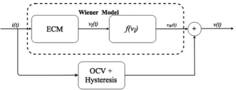
The NL-ECM model adopted in this work is presented inFig. 1 and consists of three elemental blocks, i.e., an ECM, a nonlinear

over-voltage functionfð

v

lÞand an open circuit voltage (OCV) cou-pled with hysteresis [53]. The OCV represents the equilibrium potential of the system, i.e., the potential difference between the negative and positive electrodes when no current is applied and the system is at rest. Hysteresis on the other hand accounts for dif-ferences observed in OCV measurements depending on the path taken to a particular state, i.e., whether the particular SoC was reached via a charge or discharge[60]. Hysteresis is related to ther-modynamic entropic effects, mechanical stress, and microscopic distortions within the active electrode materials following the application of an electrical load[61], [62].

The ECM, shown inFig. 2 [63], characterises the dynamics of the battery. The model structure comprises of two parallel resistor–ca-pacitor (RC) networks connected in series with a resistor. Each cir-cuit element represents a particular phenomenon governed by its respective timescales. The pure Ohmic resistanceR0comprises all

electronic resistances of the battery and corresponds to the instan-taneous voltage drop when a battery is connected to an electrical load. The charge transfer process which is attributed to the charge transfer reaction at the electrode/electrolyte interface and the double layer capacitance [3] is captured by Rp1 and Cp1 and

typically corresponds to a frequency (f) offP1Hz. Ionic diffusion in the solid phase is represented by Rp2 and Cp2 and is usually

characterised in pulse power tests as the linear (or close to linear) voltage drop and corresponds to a frequency of between 0:001Hz6f61Hz. Solid phase ionic diffusion is usually consid-ered to be the rate determining step for Li ion batteries[52]. It is noteworthy that the ECM structure presented in this paper neglects the high frequency inductive behaviour of the battery, which is known to occur at much higher frequencies, e.g., f_>300 Hz and is therefore beyond the frequency range associated with most battery management control systems.

[image:4.595.316.560.65.158.2]

The linear kinetics of the LIB is phenomenologically modelled in this paper using an ECM. Nonlinearity associated with current den-sity comprises of concentration polarisation and active polarisa-tion, which is dominant [52]. In classical electrochemistry, concentration polarisation is described by Fick’s diffusion equation

Fig. 1.The block diagram of the NL-ECM.

[image:4.595.317.556.604.739.2]

while the reaction kinetics of the battery (and thus active polarisa-tion) is modelled by the Butler-Volmer equation:

id¼i0

exp

a

aF

RT

g

exp

a

cF

RT

g

ð1Þ

whereid,

g

;i0,T,F,R;

a

aand

a

crepresent the current density, over-potential, exchange current density, temperature, Faraday constant, the universal gas constant, and the anodic and cathodic exchange coefficients, respectively. Eq. (2) combines two Tafel expressions of the form

g

¼aþblogðidÞ ð2Þ

to handle the forward and reverse reaction rates that occur at the electrode–electrolyte interface. The parametersa andbin Eq.(2) are constants, typically defined through fitting to constant current discharge curves. The Tafel expressions skew the forward or reverse reaction depending on the sign of the applied over-potential[64]. In the high over-potential regime, i.e. the Tafel regime, the Faradic reaction kinetics are nonlinear[65]. This nonlinearity is captured in the equivalent circuit formulation by a nonlinear over-voltage functionf_ð

v

lÞand takes the form[53]:

fð

v

lÞ ¼

c1

v

lðtÞ

1þc2k

v

lðtÞk ð

3Þ

where

v

lðtÞis the linear over-voltage signal andc1andc2are

sig-moid coefficients that need to be estimated. Derivation off_ð

v

lÞas well as further discussion on the form of f_ð

v

lÞcan be found in

[53], [66]. The Weiner sub-model is described in the following section.

3. Problem description for the Wiener sub-model

This section describes the Wm for the NL-ECM shown inFig. 1. The Wm is a cascade of the ECM and the nonlinear over-voltage function that represents the continuous-time linear model and output static nonlinear function, in the classical Weiner formula-tion respectively. The input to the Wm is the load current iðtÞ

and the output is the Wiener voltage, denoted by

v

WðtÞ, as shown inFig. 1. The NL-ECM can be described by three input-output rela-tionships as follows:

v

lðtÞ ¼BAðDÞðDÞiðtÞ

v

WðtÞ ¼1þcc1v2klvðtlðÞtÞk

v

ðtÞ ¼

v

wðtÞ þ

v

OCVðtÞ þeðtÞ

ð4Þ

where the currentiðtÞand the voltage

v

lðtÞare the input and output of the continuous-time linear sub-model model and the subscriptl refers to linear. The output of the continuous-time linear sub-model

v

lðtÞis the input of the output-static nonlinear function (nonlinear over-voltage function). The sigmoid function with an absolute expression is selected to describe the output static nonlinear func-tion whose output is

v

WðtÞ. The square-root expression adopted in

[53]is replaced in this work, without loss of generality, by the abso-lute expression

v

lðtÞfor simplicity in forthcoming derivations. The constantsc1andc2are real scalar weighting coefficients which

sig-nify the relative importance of the nonlinear function. The sampled form of

v

WðtÞat instancekis denoted

v

WðtkÞwheret¼kTsandTsis the sampling time. The last equation in(4)shows

v

ðtkÞas the mea-sured signal which is produced by corrupting the sum of

v

WðtkÞand the open circuit voltage

v

OCVðtkÞwith discrete white (zero mean) noise eðtkÞrepresenting the measurement noise. This process of including noise is usually known as output error, representing mea-surement noises. The continuous-time linear sub-model is described by input and output polynomials, denoted BðDÞand

AðDÞ;respectively, and are known, fromFig. 2to be second order, such that:

AðDÞ ¼a0D2_{þa1D þa} 2

BðDÞ ¼b0D2_{þb1D þb} 2

ð5Þ

whereDn_{is then}th_{order time derivative termd}n

=dtn;n2Rand the coefficientsajðj¼0;1;2Þandbjðj¼0;1;2Þare real and bounded to match the selected structure. The increase in order does not affect the derivation of the proposed algorithm.

4. Reformulation of the Wiener model for the WSRIVC method

This section illustrates how the nonlinear Wm presented in(4) can be re-arranged such that the relation betweeniðtÞand

v

WðtÞis described by a linear model which then allows any linear estimator to be used in estimating the model parameters. BothiðtÞand

v

WðtÞ are assumed to be accessible and the parameter estimation is based on the collectediðtÞand

v

WðtÞdata. The second equation in(4)can be re-arranged and expressed as:

v

WðtÞ ¼c1

v

lðtÞ c2gðtÞ ð6Þ

wheregðtÞ ¼

v

WðtÞk

v

lðtÞk. Replacing

v

lðtÞwithBAðDÞðDÞiðtÞleads to a

re-expression of(6)as:

v

WðtÞ ¼

c1BðDÞ

AðDÞ iðtÞ c2gðtÞ ð7Þ

It can readily be observed thatc1andBðDÞcan be combined without

loss of generality. For simplicityc1is assumed to be a positive real

constant. So this property can be used to reformulate(7)such that

BðDÞ ¼b0s2þb1sþb2 andgðtÞ ¼

v

WðtÞk

v

lðtÞkwhere bi¼c1bi and

v

lðtÞ ¼

BðDÞ

AðDÞ. This leads to the re-expression of(7)as:

v

WðtÞ ¼

BðDÞ

AðDÞiðtÞ cgðtÞ ð8Þ

wherec¼c2=c1.

5. SRIVC method for Wiener Sub-model (WSRIVC)

In what follows theWiener sub-modelis expressed within the framework of the simplified refined instrumental variable method for the continuous-time system identification. The Wm is re-expressed as a multi-input, single-output continuous-time model. Thus, the error function in (4), considering (8), can be expressed as:

e

WðtÞ ¼

v

ðtÞ dOCV

BðDÞ

AðDÞiðtÞ cgðtÞ

ð9Þ

where the subscriptWrefers to Wiener and the offsetdOCVis a con-stant and is introduced to approximate the open circuit voltage within an infinitesimal SoC window. The Laplace transform of (9), considering zero initial conditions, is therefore:

EWðsÞ ¼VðsÞ dOCVðsÞ

BðsÞ

AðsÞIðsÞ cGðsÞ

ð10Þ

wheredOCVðsÞ ¼1sdOCVand the Laplace transforms of the output and input polynomials, respectively, are given by:

AðsÞ ¼a0s2þa1sþa2

BðsÞ ¼b0s2þb1sþb2

ð11Þ

To approximate the derivative terms, while retaining EWðsÞon the left-hand side of (10) without filtering, a filter 1

AðsÞis introduced in

introduction of an output polynomialAðsÞin the first term of (10) as follows:

EWðsÞ ¼AðsÞ 1

AðsÞVðsÞ dOCVðsÞ ½BðsÞ 1

AðsÞIðsÞ cGðsÞ ð12Þ

Eq. (12) can then be transformed back to the time-domain and expressed as:

e

WðtÞ ¼AðDÞ 1

AðDÞ

v

ðtÞ dOCV ½BðDÞ 1

AðDÞiðtÞ cgðtÞ ð13Þ

It can be observed thatgðtÞis not filtered by 1

AðDÞ:This is because the

functiongðtÞdoes not contain derivative terms which is required for estimation. Thus, the error function in (13) is rearranged and described in a filtered form as:

e

WðtÞ ¼AðDÞ

v

FðtÞ dOCV ½BðDÞiFðtÞ cgðtÞ ð14Þ

where the subscriptFdenotes a signal filtered by 1

AðDÞ. The filtered

input and output areiFðtÞand

v

FðtÞ, respectively, and are obtained by:

iFðtÞ ¼AðDÞ1 iðtÞ

v

FðtÞ ¼_AðDÞ1

v

ðtÞ

ð15Þ

The pseudo-linear regression form can be obtained from the sam-pled form of(15)and expressed as:

D2

v

FðtkÞ ¼

u

TF;WðtkÞhWþ

e

wðtkÞ ð16Þ

wherea0¼1 and

hW¼ ½a1; a2; b0; b1; b2; c; dOCV T

ð17Þ

u

T

F;WðtkÞ ¼ ½D

v

FðtkÞ;

v

FðtkÞ; D2iFðtkÞ; DiFðtkÞ; iFðtkÞ; gðtkÞ; 1

ð18Þ

Theg_ðtkÞfunction is not directly accessible. However, sincegðtkÞis a function of

v

lðtkÞand

v

WðtkÞ, it can be simulated based on previ-ously (recent) obtained estimates. The estimated

v

^lðtkÞand^

v

WðtkÞ

can be approximated using^c; d^OCV,

v

^lðtkÞ,B^ðDÞandA^ðDÞ. In this paper, the firstB^ðD;^h1;WÞandA^ðD;^h1;WÞpolynomials are selected with the following considerations: (i) the output steady state of

the linear system, (ii) the type of linear system, whether it is under-damped or over-under-damped, and (iii) the cut-off frequency that can be selected according to the state variable filter design[67]. Similarly, the initial filter in(15)can be selected as 1

^

AðD;^h1;WÞ. The nonlinear and

offset coefficients^candd^OCVare selected to be zeros.

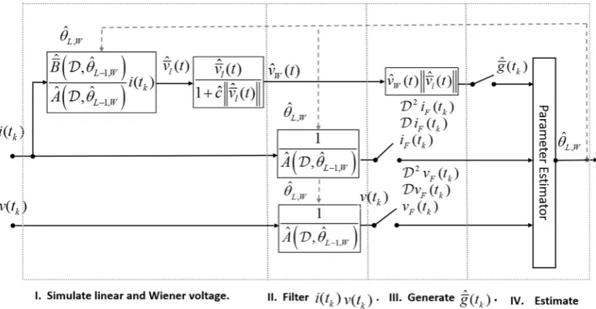
The iterative WSRIVC method is illustrated inFig. 3and its exe-cution is summarised as follows:

Simulate the noise-free output

v

^lðtÞusing:

^

v

lðtÞ ¼

^

BðD;^hL1;WÞ ^

AðD;^hL1;WÞ

iðtkÞ ð19Þ

^

v

WðtÞ ¼

^

v

lðtÞ 1þ^ck

v

^lðtÞk

ð20Þ

where

v

^lðtÞand^

v

WðtÞare used as the input to^giðtkÞ. The subscriptL indicates the current iteration number andL1 indicates the pre-vious iteration number.

Filter

v

ðtkÞandiðtkÞto generate their respective filtered forms containing higher derivatives, using:

FðDÞ ¼_^ 1

AðD;^hL1;WÞ

ð21Þ

Generate^gðtkÞin (18) using^

v

lðtÞand

v

^WðtÞ.

Obtain the estimated parameters using the LS algorithm:

^

hl;W¼ ð XN

k¼1 ^

u

F;WðtkÞ

u

^TF;WðtkÞÞ 1

XN

k¼1 ^

u

F;WðtkÞD2

v

FðtkÞ ð22Þ

where

u

^T

F;Wis defined as:

^

u

T

F;WðtkÞ ¼ ½D

v

FðtkÞ;

v

FðtkÞ; D2

v

l;FðtkÞ; D

v

l;FðtkÞ;

v

l;FðtkÞ; ^gðtkÞ; 1

ð23Þ

There is no need to use the instrumental variable regression vector because the estimatedg_ðtkÞis used as an instrumental variable.

Iterate from (I) to (IV) until the sum of the squares of the differences between ^hL1;W and ^hL;W is significantly small

[image:6.595.93.514.513.731.2]

k^hL1;W^hL;Wk<104or for a defined number of iterations. The max-imum number of iterations is selected to be 5 such that the steps (I)

to (IV) are repeated untilL= 5. This is because in a case study pre-sented later, convergence is found to occur after 3 iterations.

6. On-line parameter estimation and updating

This section presents how the off-line estimation can be extended to on-line estimation. Since the parameters can be esti-mated off-line and the model can be expressed in linear regression form, as given in (16), the off-line estimator can be extended to on-line estimation. This estimation process is divided into on-linear and nonlinear parts where the linear estimation extracts the parame-ters of the linear submodule and the nonlinear estimation part obtains the nonlinear coefficients.

For estimating the linear sub-model parameters, there is a need to estimate the linear voltage

v

^lðtkÞ, given in (20) and illustrated in

Fig. 1. The linear voltage can be estimated using the inverse of the

v

wðtkÞfunction in (20) which is expressed as:

^

v

lðtkÞ ¼

^

v

WðtkÞ

1^cðtkÞk

v

^WðtkÞk ð

24Þ

where

v

^WðtkÞ ¼

v

ðtkÞ d^OCVðtkÞ. Since the input

v

^lðtkÞand output

v

ðtkÞof the linear sub-model are realisable, the pseudo- regression form of the linear sub-model can be derived and expressed as:

D2

v

F;lðtkÞ ¼

u

TF;lðtkÞhl ð25Þ

wherea0¼1 and

hl¼ ½a1; a2; b0; b1; b2

T

ð26Þ

u

T

F;lðtkÞ ¼ ½D

v

F;lðtkÞ;

v

F;lðtkÞ; D2iFðtkÞ; DiFðtkÞ; iFðtkÞ ð27Þ

Following the classical derivation of the RLS algorithm with an inherent mechanism for tracking time-varying parameters as given in[68], the general form of RLS is expressed as:

Prediction Step:

^

hlðtkÞ ¼^hlðtk1Þ

PðtkÞ ¼Pðtk1Þ þPv ð

28Þ

Correction Step:

LðtkÞ ¼PðtkÞ

u

^F;lðtkÞð1þ

u

^TF;lðtkÞPðtkÞ

u

^F;lðtkÞÞ

1

^

hlðtkÞ ¼^hlðtkÞ þLðtkÞðD2

v

F;lðtkÞ

u

^TF;lðtkÞ^hlðtk1ÞÞ

PðtkÞ ¼ ðPðtkÞ LðtkÞ

u

^TF;lðtkÞPðtk1ÞÞ

ð29Þ

The initial values ofPð0Þare selected asPð0Þ ¼

l

Iwhere

l

>0andI is an identity matrix whileP_v¼kIand 0<k<1. In this paper, they are selected such as k¼106 _{and Pð0Þ ¼10}4 _{I. This is}

because hnð0Þ is extracted from hW which is obtained from the off-line estimation. This means there is no need for large corrections.

The sampling interval of the nonlinear estimation (TK) is 250 times slower than the linear estimation sampling interval TK¼250Tk whereTk is the sampling time of the system and is selected to beTk¼0:1sfor linear estimation. The form for the pseudo-linear regression, considering that the nonlinear parame-ters are derived from the substitution of Eq.(8)into the last equa-tion in(4), can be expressed as:

xðtKÞ ¼

u

TnðtKÞhn ð30Þ

where

xðtKÞ ¼

v

ðtKÞ

v

lðtKÞ ð31Þ

hn¼ ½c; dOCV

T _ð32Þ

u

T

nðtKÞ ¼ ½ gðtKÞ; 1 ð33Þ

The parameter vectorhnat sampleKis obtained using all data col-lected betweenK1 andKin the LS algorithm by using:

^

hnðtKÞ ¼ ð XK

k¼K1

u

nðtkÞ

u

TnðtkÞÞ 1

XK

k¼K1

u

nðtkÞxðtkÞ ð34Þ

The iterative on-line estimation process is illustrated inFig. 4and summarised as follows:

I. Use the estimated nonlinear parameters vector ^hnðtK1Þ ¼ ½^cd^OCV for estimating

v

^lðtkÞ using the inverse function in

(24)where^hnð0Þis obtained using off-line estimation. II. Filter

v

^lðtkÞandiðtkÞfor producing their filtered data using:

FðDÞ ¼_^ 1

AðD;^hL1;lðtk1ÞÞ

ð35Þ

III. Obtain the estimated parameters^hlðtkÞusing RLS given in(28) where subscriptLrefers to the iteration number.

IV. Update the parameters in the NL-ECM at the samplek. V. Steps I to IV are repeated forL= 3 iterations.

VI. Update^hnðtK1Þatt¼tK. Updating^hnðtK1Þis achieved by the

following steps:

i. Use the matrix of parameter vectors^hlðtk:KÞand^cðtK1Þto

simulate

v

^lðtÞusing:

^

v

lðtk:KÞ ¼

^

BðD;^hlðtk:KÞÞ ^

AðD;^hlðtk:KÞÞ

iðtk:KÞ ð36Þ

^

v

Wðtk:KÞ ¼ ^

v

lðtk:KÞ 1þ^cðtK1Þk

v

^lðtk:KÞk

ð37Þ

where vectors

v

^lðtk:KÞand

v

^Wðtk:KÞare used as inputs to generateg^iðtk:KÞ

ii. Obtain the estimated parameters using(34).

iii. Use ^hnðtKÞ to update the nonlinear parameters in the NL-ECM and return to step I for the next sample.

7. Results and discussion

The results obtained from the approach proposed in this paper, in terms of estimation efficiency (off-line convergence and on-line parameter estimation) and physical parameters (i.e., R0;RP1;RP2;

s

P1;

s

P2;dOCV;c), are presented in this section.

The algorithm was tested with experimental data collected from a commercial 3Ah 18650-type cell which comprises graphite negative electrode, a LiNiCoAlO2positive electrode and commercial

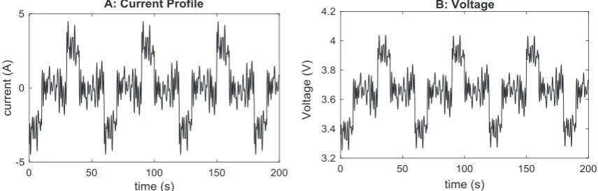
[image:7.595.300.551.636.739.2]

electrolyte. For off-line parameter estimation, data was collected at 20 different battery operating points which are the various combinations of SoC¼ ½10%;20%;50%;80%;95% and tempera-turesT¼ ½0o_C;10o_C;25o_C;45o_{C:At each operating point, a}

pulse-multisine current signal[53] is applied to the cell using a Bitrode cell cycler. The corresponding voltage response is mea-sured. An example, of the pulse-multisine current signal and the voltage response for the 3 Ah 18650 cell used in this work is shown inFig. 5. Within the figure, a positive current indicates charging while a negative current depicts discharge. For increased robust-ness of results, four different cells were tested. Thus, the algorithm was executed, off-line, 80 times.

The estimated parameters are averaged over four cells. Because the parameters are state-dependent (i.e., dependant on SoC and temperature), the obtained parameters for a given state are put into a 2D look-up table and are linearly interpolated to approxi-mate the parameters between the selected intervals.

7.1. Off-line estimator performance

The convergence of the algorithm is typically determined by the stability of the linear sub-model of the NL-ECM. The estimations of the linear sub-model obtained in all-20 iterations, for 80 runs, were found to be numerically stable. To facilitate the discussion, the results of one run – corresponding toT¼00_{CandSoC¼95%– is}

addressed in this subsection. This particular combination was chosen because at low temperatures and extreme SoC values the battery is known to exhibit strong nonlinear characteristics. Fig. 6shows that the estimates converge to acceptable values in the third iteration. The results also show that after the third itera-tion, there is no significant difference in magnitude and phase. It can also be noted that for higher frequencies (circa.

x

>2rads1_{), both phase and magnitude do not fluctuate around}

one value but both increase as the iteration number increases. This may be because the system is of much higher order.

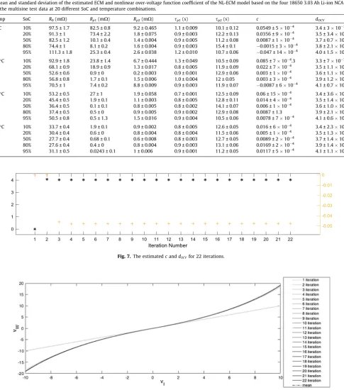
The convergence of the coefficient of the nonlinear over-potential functioncis given inTable 1. The offset parameterdOCV stabilised in the second iteration and negligibly changed as the number of iterations increased beyond 2, as shown inFig. 7. The performance of the estimated nonlinear overpotential function is shown inFig. 8. It can be seen that, apart from the first iteration which is the initial value, the performance exhibits no difference after the second iteration. These results highlight the efficiency of the estimator performance and convergence. Although the WSRIVC is modified for the nonlinear model shown inFig. 1, it pro-vides similar statistical convergence of parameters, as shown in Table 1, and frequency response, as shown in Fig. 6, to results obtained using the SRIVC method [69] which was designed for the linear system. This efficiency in convergence and frequency response mean that the proposed method can be applied online to estimate the parameters of nonlinear models with the same computational effort as traditional linear models. More investiga-tion however, is required to fully understand the higher frequency performance of the model. For this purpose, the ECM defined in Fig. 2, which is inherently limited by the bandwidth, needs to be reformulated to capture a higher frequency range, using for exam-ple, constant phase element blocks.

7.2. Identified model parameters

The proposed algorithm in this paper is used to estimate the NL-ECM parameters for a 3 Ah C6/LNiCoAlO218650 Li-ion battery

using a pre-defined set of pulse-multisine signals. The mean and standard deviation of the NL-ECM parameters R0; Rp1; Rp2

s

p1;

s

p2;c dOCV, calculated over four cells, corre-sponding to each battery state, are tabulated inTable 1. It is

note-Fig. 5.Pulse-multisine test at SoC¼50%andT¼0o

[image:8.595.89.517.408.545.2]

C. (A) The current and (B) the voltage response.

Fig. 6.Shows the logarithmic magnitude ofvl(left panel) and the phase (right panel) against frequency response of the linear sub-model for 20 iterations obtained using the

off-line WSRIVC method. The first iteration is depicted in lightest grey-line, the last iteration is presented in black-line; consecutively darker shades of grey are used for larger iteration numbers. The mean of the last ten iterations is depicted by a black-dashed-line. The multisine test data atT¼00

[image:8.595.63.547.586.722.2]

worthy to highlight that the trend ofRoinTable 1varies with SoC, contrary to what is expected by definition[3]. As previously dis-cussed in Section 2, theoretically,Rois the pure Ohmic resistance of the battery corresponding to a frequency f1Hz, while Rp1

and Rp2 are associated with the charge-transfer process

(fP1 Hz) and ionic diffusion (103_{Hz6f61 Hz), respectively.}

A major drawback of the Multisine approach, adopted in this work due to its suitability for online parameter estimation, is thatRois no longer well defined. The principal component of the driving

multisine current load isf¼1 Hz. Thus, the analogy of the ECM components with physio-chemical sub-processes are undermined. This issue is also persistent in pulse power experiments (typically f60:1 HzÞ. Nevertheless, the sum of resistances R0; Rp1; Rp2,

[image:9.595.51.537.75.626.2]

which will govern the voltage response, at all temperatures follow the general theoretical trend for cell resistance as a function of SoC. That is, the total resistance is at a minimum for circa. 50%SoC, with the highest resistances observed as SoC tends towards 0% and 100% SoC (although total resistance is higher for 0% than

Table 1

The mean and standard deviation of the estimated ECM and nonlinear over-voltage function coefficient of the NL-ECM model based on the four 18650 3.03 Ah Li-ion NCA cells, using the multisine test data at 20 different SoC and temperature combinations.

Temp SoC R0(mX) Rp1(mX) Rp2(mX) sp1(s) sp2(s) c dOCV

0°C 10% 97.5 ± 1.7 82.5 ± 0.8 9.2 ± 0.465 1.1 ± 0.009 10.1 ± 0.12 0.0549 ± 5104

3.4 ± 3103

20% 91.3 ± 1 73.4 ± 2.2 1.8 ± 0.075 0.9 ± 0.003 12.2 ± 0.13 0.0356 ± 9104 _{3.5 ± 3.410}3

50% 82.5 ± 1.2 10.1 ± 0.4 1.4 ± 0.004 0.9 ± 0.005 11.2 ± 0.08 0.0087 ± 1104

3.7 ± 0.7103

80% 74.4 ± 1 8.1 ± 0.2 1.6 ± 0.004 0.9 ± 0.003 15.4 ± 0.1 0.0015 ± 3104

3.8 ± 2.1103

95% 111.3 ± 1.8 25.3 ± 0.4 2.6 ± 0.038 1.2 ± 0.010 10.7 ± 0.06 0.047 ± 14104

4.0 ± 1.5103

10°C 10% 92.9 ± 1.8 23.8 ± 1.4 6.7 ± 0.444 1.3 ± 0.049 10.5 ± 0.09 0.085 ± 7104_{.3 3.3 ± 710}3

20% 68.1 ± 0.9 18.9 ± 0.9 1.3 ± 0.017 0.8 ± 0.005 11.9 ± 0.09 0.022 ± 7104 _{3.5 ± 1.110}3

50% 52.6 ± 0.6 0.9 ± 0 0.2 ± 0.003 0.9 ± 0.001 12.9 ± 0.06 0.003 ± 1104

3.6 ± 1.1103

80% 56.8 ± 0.8 1.7 ± 0.1 1.5 ± 0.006 1.0 ± 0.004 12 ± 0.05 0.003 ± 3104

3.9 ± 1.2103

95% 70.5 ± 1 7.4 ± 0.2 8.8 ± 0.009 0.9 ± 0.003 11.9 ± 0.07 0.0087 ± 6104

4.1 ± 0.7103

25°C 10% 53.2 ± 0.5 27 ± 1 1.9 ± 0.058 0.7 ± 0.001 12.5 ± 0.09 0.06 ± 15104 _{3.4 ± 3.610}3

20% 45.4 ± 0.5 1.9 ± 0.1 1.1 ± 0.003 0.8 ± 0.005 12.8 ± 0.11 0.014 ± 4104

3.5 ± 1.4103

50% 36.4 ± 0.5 0.1 ± 0.1 0.8 ± 0.005 0.8 ± 0.002 14.1 ± 0.07 0.006 ± 1104

3.6 ± 1.0103

80% 37.4 ± 0.5 0.5 ± 0 0.9 ± 0.005 0.9 ± 0.002 12.9 ± 0.08 0.0087 ± 1.3 3.9 ± 2.1103

95% 50.5 ± 0.8 0.5 ± 1.3 1.5 ± 0.016 0.9 ± 0.004 10.5 ± 0.06 0.0078 ± 7104

4.1 ± 0.6103

45°C 10% 33.7 ± 0.4 1.9 ± 0.1 0.9 ± 0.002 0.8 ± 0.005 12.6 ± 0.05 0.016 ± 6104

3.4 ± 2.3103

20% 30.4 ± 0.4 0.6 ± 0 0.8 ± 0.004 0.8 ± 0.004 11.5 ± 0.06 0.005 ± 1104

3.5 ± 1.3103

50% 27.7 ± 0.4 0.68 ± 0.1 0.6 ± 0.008 0.8 ± 0.003 12.7 ± 0.05 0.0089 ± 2104

3.7 ± 1.4103

80% 27.6 ± 0.4 0.4 ± 0 0.8 ± 0.004 0.9 ± 0.003 13.1 ± 0.06 0.0169 ± 2104

3.9 ± 1.4103

95% 31.1 ± 0.5 0.0243 ± 0.1 1 ± 0.006 0.9 ± 0.001 11.2 ± 0.05 0.0117 ± 5104

[image:9.595.32.552.97.329.2]

4.1 ± 1.1103

Fig. 7.The estimatedcanddOCVfor 22 iterations.

Fig. 8.Estimated nonlinear over-potential function. The multisine test data atT¼00

100% SoC) as shown in the leftmost plot inFig. 9. Moreover, the leftmost plot inFig. 9illustrates that the increase in temperature causes a reduction in all resistance parameters.

Nonlinearity, quantified byc, is found to be most significant at low SoCs and low temperatures, where ion dynamics are relatively slower. For higher values of SoC and temperatures,cis found to be small, such that

v

w¼1þcvklvlk

v

l. That is, in thec1, the shape of

the sigmoid is incentive toc:

As expected, the estimated offset parameter^dOCV is highly cor-related to the SoC such that a higher offset is obtained with higher SoC, as shown inTable 1and the rightmost plot inFig. 9. The tem-perature has an insignificant effect on the estimated offset param-eter, in agreement with previous studies[63].

Using the estimated mean parameters presented inTable 1, the NL-ECM model is validated with a charge sustaining drive-cycle current profile recorded from a prototype EV when driving in an urban environment with frequent acceleration and regenerative braking events. This highly dynamic driving cycle is employed for validation because under extended periods of high current loads, the battery enters a regime of diffusion limitation[52]where the NL extension to the linear ECM becomes significant. Such a current profile was also used for validation in[53]where the first order lin-ear ECM displayed a root-mean-square error of 3:3102under the same SoC and temperature conditions considered in this work.

As shown inFig. 10, there is very good agreement between the mea-sured and modelled voltage. The proposed model generates a root-mean-square error of 2:51102_{over 1200 s of cycling, which}

rep-resents a significant improvement from the linear case[53,63].

7.3. On-line estimation

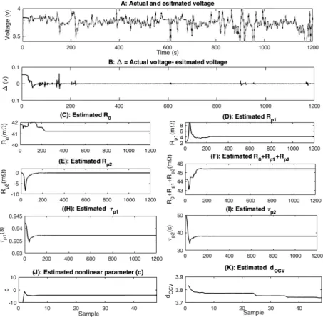
The result of on-line estimation is presented inFig. 11. The results for on-line estimation show a more accurate voltage estima-tion than its off-line counterpart, which is clearly identified by com-paring the voltage error inFigs. 10(B)–11(B). It is noteworthy that in the first 200 s a large correction occurred following which all the estimates tend to an asymptotic value. The model parameters are also shown to smoothly converge, as illustrated in Fig. 11(C–J). The accuracy of the estimates of the linear sub-model leads to an almost zero error for approximately three-quarters of the 1200 s load cycle. This was because the iterative technique used for the on-line estimation of parameters sampled at each time step, thus improving the correction. The excessive, but inexpensive, correc-tions to the parameter estimates caused a minimisation of the error between the modelled and actual voltages.

[image:10.595.70.532.341.501.2]

Because the error between the modelled and actual voltages is zero after the first circa. 200 s, the nonlinear coefficient was not subject to significant corrections, as shown inFig. 11(J). This is

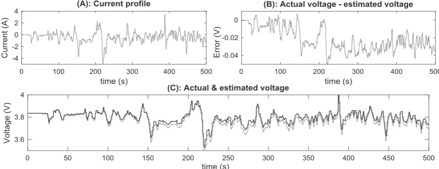
[image:10.595.75.528.553.728.2]

Fig. 10.Validation results of current drive cycle for first 500 s of the 1200 s at 70% SoC and temperature at 10°C in (A) and the difference between measured and modelled voltage in (B) and measured and model voltage in (C) and presented in black and grey, respectively.

Fig. 9.Sum of the resistance elements in the NL-ECM is presented on the left-side, the estimated nonlinear coefficient^cis located on the middle andd^OCVplot is on the

because the correction factor is a function of error. The charge sus-taining drive cycle used to demonstrate on-line parameter estima-tion consumed a total of 6% SoC (from a starting SoC of 70%). For the commercial battery considered in this study, this change in SoC corresponds to an OCV change of more than 70 mV.

8. Conclusions and further work

8.1. Conclusions

In this paper, a novel algorithm is proposed that directly esti-mates the model parameters of a nonlinear equivalent circuit model from observed input–output data. The parameter estima-tion algorithm extends the simplified refined instrumental variable method to estimate the Wiener model, which itself was reformu-lated into a multi-input/single-output linear model using a static nonlinear function (i.e., sigmoid function) that characterises the

nonlinear voltage response of a LIB under a diffusion limited regime. A recursive least squares algorithm was then employed for parameter estimation.

The iterative offline estimation algorithm is extended to an iter-ative online estimation. The online estimation is divided into two sub-estimators. The first estimator extracts the parameters of the linear sub-model and executes at timescales within the sampling timescale of collected data. The second sub-estimator obtains the coefficient of the nonlinear static function and the offset and runs after a pre-defined number of samples.

Both on-line and off-line approaches were applied to a commercially available 3Ah C6/LNiCoAlO2 18650-type cell using

[image:11.595.66.520.67.515.2]

pulse-multisine tests. The extracted parameters were then validated using a charge sustaining drive-cycle recorded from a prototype electric vehicle driving in an urban environment. Both the on-line and off-line validation results showed very good agree-ment with measured terminal voltage. The parameter estimation

Fig. 11.The results of on-line estimation and prediction of NL-ECM with the same validation profile, shown inFig. 10where (A) shows the predicted and actual voltages, (B) gives the error between the actual and estimated voltages (C–F) present the resistance in the NL-ECM in a form ofR0,Rp1Rp2andR0þRp1þRp2, respectively, (G, H) are the

time constantssp1andsp2, respectively and (I, J) show the estimated nonlinear coefficientcand offsetdOCV, respectively, for 48 samples because estimation of the nonlinear

algorithm for the nonlinear battery model proposed in this work exhibited fast convergence, similar to that demonstrated with lin-ear models[69], which is advantageous for on-line BMS applica-tions. In addition, the algorithm depends only on the on-board available signals, i.e., the battery terminal voltage and current mea-surements, and thus is suitable for EV applications. The low model complexity and the efficient recursive algorithm can facilitate real time implementation.

8.2. Further work

The model was validated using short-term drive cycle data, so it is difficult to assess how the model will adapt to changes in battery characteristics due to the aging process. Future work will thus focus on state of health estimation, in particular assessing the algo-rithm response to battery degradation. In addition to SoH, it will also be of interest to investigate the possibility of using this, more accurate identification procedure, for OCV estimation and hence online SoC estimation.

Acknowledgements

This research was supported by the Engineering and Physical Science Research Council grants EP/M507143/1, EP/N001745/1 and EP/P511432/1.

References

[1]Wang Y, Chen Z, Zhang C. On-line remaining energy prediction: a case study in

embedded battery management system. Appl Energy 2017;194:688–95.

[2]Marongiu A, Nußbaum FGW, Waag W, Garmendia M, Sauer DU.

Comprehensive study of the influence of aging on the hysteresis behavior of a lithium iron phosphate cathode-based lithium ion battery – an experimental

investigation of the hysteresis. Appl Energy 2016;171:629–45.

[3]Waag W, Käbitz S, Sauer DU. Experimental investigation of the lithium-ion

battery impedance characteristic at various conditions and aging states and its

influence on the application. Appl Energy 2013;102(Feb):885–97.

[4]Vetter J, Novák P, Wagner MR, Veit C, Möller K-C, Besenhard JO, Winter M,

Wohlfahrt-Mehrens M, Vogler C, Hammouche A. Ageing mechanisms in

lithium-ion batteries. J Power Sources 2005;147(1):269–81.

[5] K. Uddin, S. Perera, W. Widanage, L. Somerville, J. Marco, Characterising lithium-ion battery degradation through the identification and tracking of electrochemical battery model parameters, Batteries, vol. 2, no. 2. Multidisciplinary Digital Publishing Institute, p. 13, Apr-2016.

[6]Uddin K, Moore AD, Barai A, Marco J. The effects of high frequency current

ripple on electric vehicle battery performance. Appl Energy

2016;178:142–54.

[7]Uddin K, Somerville L, Barai A, Lain M, Ashwin TR, Jennings P, Marco J. The

impact of high-frequency-high-current perturbations on film formation at the

negative electrode-electrolyte interface. Electrochim Acta 2017.

[8]Cannarella J, Arnold CB. State of health and charge measurements in

lithium-ion batteries using mechanical stress. J Power Sources 2014;269:7–14.

[9]Xing Y, Ma EWM, Tsui KL, Pecht M. Battery management systems in electric

and hybrid vehicles. Energies 2011;4(12):1840–57.

[10]Lu L, Han X, Li J, Hua J, Ouyang M. A review on the key issues for lithium-ion

battery management in electric vehicles. J Power Sources 2013;226:272–88.

[11]Zhang J, Lee J. A review on prognostics and health monitoring of Li-ion battery.

J Power Sources 2011;196(15):6007–14.

[12]Pop V, Bergveld HJ, Notten PHL, Regtien PPL. State-of-the-art of battery

state-of-charge determination. Meas Sci Technol Dec. 2005;16(12):R93–R110.

[13]Rahimi-Eichi H, Ojha U, Baronti F, Chow M-Y. Battery management system: an

overview of its application in the smart grid and electric vehicles. IEEE Ind

Electron Mag 2013;7(2):4–16.

[14]Xia B, Zhao X, de Callafon R, Garnier H, Nguyen T, Mi C. Accurate Lithium-ion

battery parameter estimation with continuous-time system identification

methods. Appl Energy Oct. 2016;179:426–36.

[15]Wei Z, Lim TM, Skyllas-Kazacos M, Wai N, Tseng KJ. Online state of charge and

model parameter co-estimation based on a novel multi-timescale estimator

for vanadium redox flow battery. Appl Energy 2016;172:169–79.

[16]Duong V-H, Bastawrous HA, Lim K, See KW, Zhang P, Dou SX. Online state of

charge and model parameters estimation of the LiFePO4battery in electric

vehicles using multiple adaptive forgetting factors recursive least-squares. J

Power Sources 2015;296:215–24.

[17]Dai H, Xu T, Zhu L, Wei X, Sun Z. Adaptive model parameter identification for

large capacity Li-ion batteries on separated time scales. Appl Energy

2016;184:119–31.

[18]Tong S, Klein MP, Park JW. On-line optimization of battery open circuit voltage

for improved state-of-charge and state-of-health estimation. J Power Sources

2015;293:416–28.

[19]He H, Xiong R, Guo H. Online estimation of model parameters and

state-of-charge of LiFePO4 batteries in electric vehicles. Appl Energy 2012;89

(1):413–20.

[20] Berecibar M, Devriendt F, Dubarry M, Villarreal I, Omar N, Verbeke W, Van

Mierlo J. Online state of health estimation on NMC cells based on predictive

analytics. J Power Sources 2016;320:239–50.

[21]Chen Z, Mi CC, Fu Y, Xu J, Gong X. Online battery state of health estimation

based on Genetic Algorithm for electric and hybrid vehicle applications. J

Power Sources 2013;240:184–92.

[22]Fleischer C, Waag W, Heyn H-M, Sauer DU. On-line adaptive battery

impedance parameter and state estimation considering physical principles in reduced order equivalent circuit battery models: Part 1. Requirements, critical

review of methods and modeling. J Power Sources 2014;260:276–91.

[23]Howey DA, Mitcheson PD, Yufit V, Offer GJ, Brandon NP. Online measurement

of battery impedance using motor controller excitation. IEEE Trans Veh

Technol 2014;63(6):2557–66.

[24]Alavi SMM, Birkl CR, Howey DA. Time-domain fitting of battery

electrochemical impedance models. J Power Sources 2015;288:345–52.

[25]Verbrugge M, Frisch D, Koch B. Adaptive energy management of electric and

hybrid electric vehicles. J Electrochem Soc 2005;152(2):A333.

[26]Verbrugge M, Koch B. Generalized recursive algorithm for adaptive

multiparameter regression. J. Electrochem. Soc. 2006;153(1):A187.

[27]Verbrugge M. Adaptive, multi-parameter battery state estimator with

optimized time-weighting factors. J Appl Electrochem 2007;37(5):605–16.

[28]Juang LW, Kollmeyer PJ, Jahns TM, Lorenz RD. System identification-based

lead-acid battery online monitoring system for electric vehicles. In: IEEE

energy conversion congress and exposition 2010. p. 3903–10.

[29]Hu X, Sun F, Zou Y. Online model identification of lithium-ion battery for

electric vehicles. J Cent South Univ Technol Oct. 2011;18(5):1525–31.

[30] Lee J, Kim Y, Cha H. A new battery parameter identification considering

current, SOC and Peukert’s effect for hybrid electric vehicles. In: IEEE Energy

Conversion Congress and Exposition 2011. p. 1489–94.

[31]Wang S, Verbrugge M, Wang JS, Liu P. Multi-parameter battery state estimator

based on the adaptive and direct solution of the governing differential

equations. J Power Sources 2011;196(20):8735–41.

[32]Roscher MA, Bohlen OS, Sauer DU. Reliable state estimation of multicell

lithium-ion battery systems. IEEE Trans Energy Convers Sep. 2011;26(3):737–43.

[33]Mandal LP, Cox RW. A transient-based approach for estimating the electrical

parameters of a lithium-ion battery model. In: IEEE Energy Conversion

Congress and Exposition 2011. p. 2635–40.

[34]Sabatier J, Aoun M, Oustaloup A, Grégoire G, Ragot F, Roy P. Fractional system

identification for lead acid battery state of charge estimation. Sig Proc 2006;86

(10):2645–57.

[35]Dai H, Wei X, Sun Z, Wang J, Gu W. Online cell SOC estimation of Li-ion battery

packs using a dual time-scale Kalman filtering for EV applications. Appl Energy

2012;95:227–37.

[36]Plett GL. Sigma-point Kalman filtering for battery management systems of

LiPB-based HEV battery packs: Part 2: Simultaneous state and parameter

estimation. J Power Sources 2006;161(2):1369–84.

[37]Haifeng Dai, Xuezhe Wei, Zechang Sun. A new SOH prediction concept for the

power lithium-ion battery used on HEVs. In: IEEE Vehicle Power and

Propulsion Conference 2009. p. 1649–53.

[38] Xiong R., Sun F., Chen Z., He H. A data-driven multi-scale extended Kalman filtering based parameter and state estimation approach of lithium-ion polymer battery in electric vehicles; 2014.

[39]Do Dinh Vinh, Forgez C, El Kadri Benkara K, Friedrich G. Impedance observer

for a li-ion battery using kalman filter. IEEE Trans Veh Technol 2009;58 (8):3930–7.

[40] Zhang Q, White RE. Calendar life study of Li-ion pouch cells. J Power Sources

2007;173(2):990–7.

[41]Samadi MF, Alavi SMM, Saif M. Online state and parameter estimation of the

Li-ion battery in a Bayesian framework. In: American Control Conference 2013. p. 4693–8.

[42]Xiong R, Yu Q, Wang LY, Lin C. A novel method to obtain the open circuit

voltage for the state of charge of lithium ion batteries in electric vehicles by using H infinity filter. Appl Energy 2017.

[43]Chen C, Sun F, Xiong R, He H. A novel dual H infinity filters based battery

parameter and state estimation approach for electric vehicles application.

Energy Proc 2016;103:375–80.

[44] Fei Zhang, Guangjun Liu, Lijin Fang, A battery state of charge estimation method using sliding mode observer. In: 2008 7th world congress on intelligent control and automation; 2008, p. 989–994.

[45]Kim I-S. The novel state of charge estimation method for lithium battery using

sliding mode observer. J Power Sources Dec. 2006;163(1):584–90.

[46]Zhang C, Wang LY, Li X, Chen W, Yin GG, Jiang J. Robust and adaptive

estimation of state of charge for lithium-ion batteries. IEEE Trans Ind Electron

Aug. 2015;62(8):4948–57.

[47]Forman JC, Moura SJ, Stein JL, Fathy HK. Genetic identification and fisher

identifiability analysis of the Doyle–Fuller–Newman model from experimental

cycling of a LiFePO4 cell. J Power Sources 2012;210:263–75.

[49] Moura SJ., Krstic M., Chaturvedi NA. Adaptive PDE Observer for Battery SOC/ SOH Estimation. In: Volume 1: adaptive control; advanced vehicle propulsion systems; aerospace systems; autonomous systems; battery modeling; biochemical systems; control over networks; control systems design; cooperativ; 2012. p. 101–10.

[50] Klein R., Chaturvedi NA., Christensen J., Ahmed J., Findeisen R., Kojic A. State estimation of a reduced electrochemical model of a lithium-ion battery. In: Proceedings of the 2010 American control conference; 2010. p. 6618–23.

[51]Xing Y, He W, Pecht M, Tsui KL. State of charge estimation of lithium-ion

batteries using the open-circuit voltage at various ambient temperatures. Appl

Energy 2014;113:106–15.

[52]Smith K, Wang C-Y. Solid-state diffusion limitations on pulse operation of a

lithium ion cell for hybrid electric vehicles. J Power Sources 2006;161 (1):628–39.

[53]Widanage WD, Barai A, Chouchelamane GH, Uddin K, McGordon A, Marco J,

Jennings P. Design and use of multisine signals for Li-ion battery equivalent

circuit modelling. Part 2: Model estimation. J Power Sources 2016;324.

[54]Vörös J. An iterative method for hammerstein-wiener systems parameter

identification. J Electr Eng 2004;55:11–2.

[55]Vörös J. Parameter identification of Wiener systems with multisegment

piecewise-linear nonlinearities. Syst Control Lett Feb. 2007;56(2):99–105.

[56]Zhou L, Li X, Pan F. Least-squares-based iterative identification algorithm for

Wiener nonlinear systems. J Appl Math May 2013;2013:1–6.

[57]Wang D, Ding F. Least squares based and gradient based iterative identification

for Wiener nonlinear systems. Signal Processing May 2011;91(5):1182–9.

[58]Chaudhary NI, Raja MAZ. Identification of Hammerstein nonlinear ARMAX

systems using nonlinear adaptive algorithms. Nonlinear Dyn 2015;79 (2):1385–97.

[59]Aslam MS, Chaudhary NI, Raja MAZ. A sliding-window approximation-based

fractional adaptive strategy for Hammerstein nonlinear ARMAX systems.

Nonlinear Dyn. 2017;87(1):519–33.

[60]Barai A, Widanage WD, Marco J, McGordon A, Jennings P. A study of the open

circuit voltage characterization technique and hysteresis assessment of

lithium-ion cells. J Power Sources 2015;295:99–107.

[61]Roscher MA, Sauer DU. Dynamic electric behavior and open-circuit-voltage

modeling of LiFePO4-based lithium ion secondary batteries. J Power Sources

2011;196(1):331–6.

[62]Verbrugge M, Tate E. Adaptive state of charge algorithm for nickel metal

hydride batteries including hysteresis phenomena. J Power Sources 2004;126 (1):236–49.

[63]Uddin K, Picarelli A, Lyness C, Taylor N, Marco J. An acausal Li-ion battery pack

model for automotive applications. Energies 2014;7(9):5675–700.

[64] Ferguson TR. Lithium-ion battery modeling using non-equilibrium thermodynamics. Massachusetts Institute of Technology; 2014.

[65]Grens EA, Tobias CW. The influence of electrode reaction kinetics on the

polarization of flooded porous electrodes. Electrochim Acta 1965;10 (8):761–72.

[66]Widanage WD, Barai A, Chouchelamane GH, Uddin K, McGordon A, Marco J,

Jennings P. Design and use of multisine signals for Li-ion battery equivalent

circuit modelling. Part 1: Signal design. J Power Sources 2016;324.

[67] Ljung L. System identification. Theory for the user. Prentice-Hall; 1987. [68] Honig ML., Messerschmitt DG. Adaptive filters: structures, algorithms, and

applications. Kluwer; 1984.