Original citation:
Bruna, Maria, Burger, Martin, Ranetbauer, Helene and Wolfram, Marie-Therese. (2016)
Cross-diffusion systems with excluded-volume effects and asymptotic gradient flow
structures. Journal of Nonlinear Science.
Permanent WRAP URL:
http://wrap.warwick.ac.uk/83896
Copyright and reuse:
The Warwick Research Archive Portal (WRAP) makes this work of researchers of the
University of Warwick available open access under the following conditions.
This article is made available under the Creative Commons Attribution 4.0 International
license (CC BY 4.0) and may be reused according to the conditions of the license. For more
details see:
http://creativecommons.org/licenses/by/4.0/
A note on versions:
The version presented in WRAP is the published version, or, version of record, and may be
cited as it appears here.
DOI 10.1007/s00332-016-9348-z
Cross-Diffusion Systems with Excluded-Volume Effects
and Asymptotic Gradient Flow Structures
Maria Bruna1 · Martin Burger2 ·
Helene Ranetbauer3 · Marie-Therese Wolfram3,4
Received: 24 July 2016 / Accepted: 25 October 2016
© The Author(s) 2016. This article is published with open access at Springerlink.com
Abstract In this paper, we discuss the analysis of a cross-diffusion PDE system for a mixture of hard spheres, which was derived in Bruna and Chapman (J Chem Phys 137:204116-1–204116-16,2012a) from a stochastic system of interacting Brownian particles using the method of matched asymptotic expansions. The resulting cross-diffusion system is valid in the limit of small volume fraction of particles. While the system has a gradient flow structure in the symmetric case of all particles having the same size and diffusivity, this is not valid in general. We discuss local stability and global existence for the symmetric case using the gradient flow structure and entropy variable techniques. For the general case, we introduce the concept of an asymptotic gradient flow structure and show how it can be used to study the behavior close to equilibrium. Finally, we illustrate the behavior of the model with various numerical simulations.
Keywords Nonlinear parabolic equations·Interacting particle systems·Asymptotic expansion·Cross diffusion·Size exclusion·Entropy techniques and gradient flow structure
Communicated by Charles Doering.
B
Marie-Therese Wolfram [email protected]1 Mathematical Institute, University of Oxford, RQQ, Woodstock Road, Oxford OX2 6GG, UK 2 Institut für Numerische und Angewandte Mathematik and Cells in Motion Cluster of Excellence,
Westfälische Wilhelms Universität Münster, Einsteinstrasse 62, 48149 Münster, Germany
Mathematics Subject Classification 35K55·35C20·60J70·82C22·35A01· 37B25
1 Introduction
Systems of interacting particles can be observed in biology (e.g., cell popula-tions), physics or social sciences (e.g., animal swarms or large pedestrian crowds). Macroscopic models describing the individual interactions of these particles among themselves as well as their environment lead to complex systems of differential equa-tions (cf. e.g.,Bendahmane et al. 2009;Bruna and Chapman 2012a,b;Burger et al. 2010,2016,2012;Di Francesco and Fagioli 2016;Painter 2009;Schlake 2011; Simp-son et al. 2009). In microscopic models, the dynamics of each particle is accounted for explicitly, while the macroscopic models typically consist of partial differential equations for the population density. Passing from the microscopic model to the macro-scopic equations in a systematic way is, in general, very challenging, and often one relies on closure assumptions, which can be made rigorous under certain scaling assumptions on the number and size of particles. In particular, when crowding due to the finite size of particles is included in the model, the limiting process is quite sub-tle and, using different assumptions and closure relations, a variety of macroscopic equations have been derived. For instance, the macroscopic equations of a two-species system where particles undergo a simple exclusion process on a lattice can be derived using formal Taylor expansions, see for exampleBurger et al.(2010),Simpson et al.
(2009). The case when particles are not confined to a regular lattice and undergo instead a Brownian motion with hardcore interactions was considered inBruna and Chapman(2012a) using matched asymptotic expansions. Cross-diffusion is a com-mon feature of all these models and poses a particular challenge for the analysis since maximum principles do not hold. Classical examples of cross-diffusion systems are reaction diffusion systems or systems describing multicomponent gas mixtures. These quasi-linear parabolic systems were analyzed byLadyzhenskaia et al.(1968) orAmann(1985,1989), which however rely on strong parabolicity assumptions that break down for the degenerate cross-diffusion systems derived from the interacting particle systems mentioned above.
The canonical form for a two-species system of interacting particles (called red and blue in the following) is
∂t
r b
= ∇ ·
D(r,b)∇
r b
−F(r,b)
r b
, (1)
where D=D(r,b)is the diffusion matrix andF =F(r,b)is the drift matrix due to a convective flux.
Systems like (1) often have a gradient flow structure
∂t
r b
= ∇ ·
M(r,b)∇
∂rE ∂bE
whereMis a mobility matrix and∂rEand∂bE denote the functional derivative of an
entropy functionEwith respect torandb, respectively. The gradient flow formulation provides a natural framework to study the analytic behavior of such systems, cf. e.g.,
Ambrosio et al.(2008). It has been used to analyze existence and long-time behavior of systems, see for exampleCarrillo et al.(2014),Jüngel and Zamponi(2014),Liero and Mielke(2013),Zinsl and Matthes(2015). As a result, being able to express a PDE system as gradient flows of an entropy is a very desirable feature; yet, this is not possible in general. The lack of the gradient flow structure on the PDE level can result from the approximations made when passing from the microscopic description to the macroscopic equations. This is the case of the cross-diffusion system derived inBruna and Chapman(2012a), which was derived using the method of matched asymptotics. There has been a lot of research on the passage from microscopic models to the continuum equations, for example in the hydrodynamic limit (Kipnis and Landim 2013). More recently, the microscopic origin of entropy structures, which connects gradient flows and the large deviation principle, was analyzed inAdams et al.(2011),
Liero et al.(2015).
In this paper, we introduce the idea of an asymptotic gradient flow structure as a generalization of a standard or, as we also call it, full gradient flow structure for systems derived as an asymptotic expansion such as that in Bruna and Chapman
(2012a). In this paper, we provide several analytic results for these cross-diffusion systems and introduce the notion of asymptotic gradient flows. We discuss how the closeness of these asymptotic gradient flow structures can be used to analyze the behavior of the system close to equilibrium. Furthermore, we present a global in time existence result in the case of particles of same size and diffusivity (in which the system has a full gradient flow structure). The existence proof is based on an implicit Euler discretization and Schauder’s fixed point theorem. We study the linearized system with an additional regularization term in the entropy to ensure boundedness of the solutions and deduce existence results for the unregularized system in the limit (similar to the deep quench limit for the Cahn Hilliard equationElliott and Garcke 1996). This is, to the authors’ knowledge, the first global in time existence result for this system so far. We note, however, that it is only valid if the total density stays strictly below a certain threshold. It relates to the fact that the model assumptions break down if the maximum density is reached. We discuss this problem in more detail in Sect.
3.
This paper is organized as follows: we introduce the mathematical model in Sect.2
2 The Mathematical Model
In this paper, we analyze a cross-diffusion system for a mixture of hard spheres derived inBruna and Chapman(2012a), which we present below. The system is obtained as the continuum limit of a stochastic system with two types of interacting Brownian particles, referred to as red and blue particles. In particular, we considerNrred particles of diameter r, constant diffusion coefficient Dr and external potentialVr˜, and Nb
blue particles of diameterb, diffusion coefficientDband external potentialVb˜ . Each
particle evolves according to a stochastic differential equation (SDE) with independent Brownian dynamics and interacts with the other particles in the system via hardcore collisions. This means that the centers of two particles with positionXiandXjin space
are not allowed to get closer than the sum of their radii, that is,Xi−Xj ≥(i+j)/2,
whereidenotes the radius of theith particle. We define the total number of particles in the system byN = Nr+Nb, and the distance at contact between a red and blue particles bybr =(r+b)/2. The situation detailed above can be described by the
overdamped Langevin SDEs
dXi(t)=
2DrdWi(t)− ∇ ˜Vr(Xi)dt 1≤i ≤ Nr,
dXi(t)=
2DbdWi(t)− ∇ ˜Vb(Xi)dt Nr+1≤i ≤N,
(3)
where Xi ∈ ⊂ Rd,d = 2,3, is the position of the ith particle andWi a d
-dimensional standard Brownian motion. We assume thatis a bounded domain. The boundary conditions due to collisions between particles and with the domain walls are
(dXi−dXj)·n=0, on Xi−Xj =(i +j)/2,
dXi·n=0, on ∂,
(4)
wherendenotes the outward unit normal. The continuum-level model associated to this individual-based model was derived inBruna and Chapman(2012a) using the method of matched asymptotic expansions in the limit of low but finite volume fraction. If
vd()is the volume of ad-dimensional ball of diameter, then the volume fraction in the system is
=Nrvd(r)+Nbvd(b), (5)
assuming that the problem is nondimensionalized such that the domainhas unit volume, || = 1. Because particles cannot overlap each other, in addition to the global constraint1 there is also a local constraint on the total volume density, defined as
φ(x,t)=vd(r)r(x,t)+vd(b)b(x,t), (6)
wherer =r(x,t)andb=b(x,t)are the number densities of the red and blue species, respectively, depending on space and time. This means thatr = Nrrˆ andb = Nbbˆ
for the probability densitiesrˆ,bˆ. Consequently, meaningful solutions satisfyr ≥ 0 withrdx=Nrandb≥0 withbdx=Nb. For more detailed information, see
the theoretical maximum allowed volume fraction, given by the Kepler conjecture. We note thatandφare related via=φdx.
The cross-diffusion model inBruna and Chapman(2012a) is valid for any number of blue and red particles,NbandNr. However, here we will consider the case that the number of both particles is large, such thatNr−1≈Nr,Nb−1≈Nb, as it simplifies the model slightly. In this case, the model reads (Bruna and Chapman 2012a)
∂tr =Dr∇ ·
(1+drαr)∇r+ ∇Vrr+brd βrr∇b−γrb∇r+ ∇(γbVb−γrVr)r b
,
(7a)
∂tb=Db∇ ·
(1+bdαb)∇b+ ∇Vbb+brd βbb∇r−γbr∇b+ ∇ γrVr−γbVb
r b,
(7b)
whereVi = ˜Vi/Diare the rescaled potentials, and the parametersα,βi andγidepend
on the geometry of the particles. For balls, they are given by
α= 2(d−1)π
d , βi =
2π
d
[(d−1)Di+d Dj]
Dr+Db , γi =
2π
d
Di
Dr+Db, (8)
fori = r,j = band vice versa, and space dimensiond = 2 or 3. This system is an asymptotic expansion inr,b (assuming that both small parameters are of the
same asymptotic order,r∼b∼), valid up to orderd. The nonlinear terms in (7)
correspond to the leading-order contribution of the pairwise particle interactions. The asymptotic method used inBruna and Chapman(2012a) could be extended if desired to evaluate higher-order terms coming from three or more particle interactions, as well as order corrections in the pairwise interaction. This would result in higher-order terms ini in (7) (of orderi(d+1)and higher) with quite some effort. However, it seems impossible to derive the full infinite series expansion.
We will consider the system (7) in×(0,T)with no-flux boundary conditions
0=n·
(1+rdαr)∇r+ ∇Vrr+brd
βrr∇b−γrb∇r+ ∇(γbVb−γrVr)r b
,
(9a)
0=n·
(1+bdαb)∇b+ ∇Vbb+brdβbb∇r−γbr∇b+ ∇ γrVr−γbVb
r b,
(9b)
on∂×(0,T)and initial values
r(x,0)=r0(x), b(x,0)=b0(x). (10)
flow, namely anasymptotic gradient flow, motivated by the underlying structure of the general system (7).
2.1 Cross-Diffusion System for Particles of the Same Size and Diffusivity
In this section, we suppose that red and blue particles are of the same size, that is
r = b := , and have the same diffusion coefficient, Dr = Db. Without loss
of generality, we take the diffusion coefficient equal one (this can be achieved by rescaling time). In this case, the cross-diffusion system (7) can be written as
∂tr = ∇ ·
(1+αdr−γ db)∇r+βdr∇b+r∇Vr+γ d∇(Vb−Vr)r b
,
(11a)
∂tb= ∇ ·
(1+αdb−γ dr)∇b+βdb∇r+b∇Vb+γ d∇(Vr−Vb)r b
,
(11b)
where βi andγi, fori = r,b, are now equal and simplify to γ = π/d andβ = 2(d−1)γ, respectively.
This cross-diffusion system can be used to describe a mixture of particles that are physically identical but that are driven by different potentialsVrandVb(for example cells that are attracted to different food sources, or pedestrians that want to move in different directions). Moreover, it can also be used to model the scenario where the red and the blue particles are in fact identical, but one has knowledge about the initial distributions of each sub-population,r0andb0. This is the scenario in many experimental setups that use noninvasive fluorescent tagging. On the other hand, if the red and blue particles are identical and initially indistinguishable, then one has thatr/Nr =b/Nb:= pfor all times. In this case, both Eqs. (11a) and (11b) reduce to the same equation, which coincides with the equation for the evolution of a single population of hard spheres as expected (Bruna and Chapman 2012b).
In the following, we defineα¯ =dα,γ¯ =dγ, and the total number density
ρ(x,t):=r(x,t)+b(x,t). (12)
When particles have the same size and diffusivity we find that
ρ≡2φ/γ ,¯ (13)
whereφis the total volume density given in (6). Usingρ, the Eq. (11) can be rewritten in the following form
∂tr= ∇ ·(1− ¯γ ρ)∇r+(α¯+ ¯γ )r∇ρ+r∇Vr+ ¯γ∇(Vb−Vr)r b, (14a)
where we have used thatβ =α+γ. It is straightforward to see that the system (14) has a formal gradient flow structure, with an entropy functional given by
E(r,b)=
rlogr+blogb+r Vr+bVb+ ¯
α
2
r2+2r b+b2
dx. (15)
Using the corresponding entropy variables
u:=∂rE=logr+ ¯αρ+Vr,
v:=∂bE =logb+ ¯αρ+Vb, (16)
the system can be written in the form
∂t
r b
= ∇ ·
M(r,b)∇
u v
, (17)
with the symmetric mobility matrix
M(r,b)=
r(1− ¯γb) γ¯r b
¯
γr b b(1− ¯γr)
. (18)
2.2 Cross-Diffusion System for Particles of Different Size and Diffusivity
In this section, we attempt to write a gradient flow structure for the general cross-diffusion system (7) guided by the symmetric case in the previous subsection, (15) and (18). We will see that this requires a generalization of the definition of gradient flow structure. We define the following entropy
E(r,b)=
rlogr+blogb+r Vr+bVb+
α
2
d
r r2+2brd r b+dbb2
dx,
(19a)
and mobility matrix
M(r,b)=
Drr(1−γrbrdb) Drγbdbrr b
Dbγrbrdr b Dbb(1−γbbrdr)
. (19b)
As mentioned earlier, we suppose that the red and blue particle sizes are of the same asymptotic order, namelyr ∼ b. It is then convenient to introduce a single small
parameter, and the order one parametersar,abandabr such thatdi =aid. Note
that asbr =(r+b)/2, it holds thatabr =((ab1/d+ar1/d)/2)d. Then, the entropy
E0=
rlogr+blogb+r Vr+bVbdx, E1=
α
2
arr
2+
2abrr b+abb2dx,
M0=diag(Drr,Dbb), M1=abrr b
−Drγr Drγb
Dbγr −Dbγb
.
(20)
Using (19), the general cross-diffusion system (7) can be rewritten as
∂t
r b
= ∇ ·
M∇
∂rE ∂bE
−2d
G
, (21)
whereG(r,b)is the vector
G=αabrr b
γr(θr∇r−θb∇b) γb(θb∇b−θr∇r)
, (22)
with
θr=Dbabr−Drar, θb=Drabr−Dbab. (23)
Then, it is easy to see that the gradient flow structure induced by (19) and our system (7) [or (21)] agree up to orderd, which is the order of the asymptotic expansion that produced (7) in the first place. In other words, the discrepancy between the system (7) and the gradient flow induced by (19) is of order2d. Therefore, up to orderd, we can see (21) as a gradient flow structure of our system. We will call this an asymptotic gradient flow structure; the precise definition will be made clear in the following section.
Finally, we note that the system (19) coincides with the gradient flow structure in the caseDr=Dbandr=b, see (15) and (18). Note thatG≡0 for the parameter
values of the simpler system (11), as expected. Specifically, we find that ifDr= Db
andr =b, thenθr =θb=0. A natural question to ask is whether there are other
parameter values for whichG(r,b)≡0 for allr,b. Imposing thatθr =θb=0 leads
to the conditiona2br =arab, which in turn leads tor =b, and thus thatDr = Db.
Therefore, the only case for which (19) is an exact gradient flow for the system is the case which we have already studied, that is when the particle sizes and diffusivities are equal.
3 Gradient Flows and Asymptotic Gradient Flows Close to Equilibrium
In the following, we provide a more detailed discussion on gradient flow structures and implications for the behavior close to equilibrium.
3.1 Full Gradient Flow Structure Case
equilibrium solutions and studying the stability and well posedness of the system close to this equilibrium solution.
We have seen in the previous subsection that the linear stability analysis for gradient flow structures reduces to showing that the mobility matrixM is positive definite in the case of a strictly convex entropy functionalE, cf.Schlake(2011). We assume from now on:
(AI) LetVr,Vb∈ H1()∩L∞().
We recall that in case of assumption (AI) an equilibrium solution(r∞,b∞)exists and that the corresponding entropy variablesu∞andv∞are constant. The determinant of the mobility matrixM defined in (18) is given by
detM =r b(1− ¯γ ρ). (24)
Together with the positivity of diagonal entries we see thatM is positive definite if
ρ <1/γ¯. This constraint gives a local bound on the total local volume density (using (13)), namely 2φ <1. This is consistent with the asymptotic assumption thatφ1. Hence, we define the set
S =
r b
∈R2:
r≥0,b≥0,r+b≤ 1
γ
, (25)
which we will also use in the existence proof presented in Sect.5. For stability and uniqueness, it will be crucial to have solutions staying strictly in the interior ofS, due to the degeneracy of the mobility matrix on the boundary ofS.
Theorem 3.1 (Linear stability)The stationary solutions of the system(17)are unique
and linearly stable with respect to small perturbationsξ, η∈ L2(0,T;H1())with
zero mean.
Proof Due to the gradient flow structure, any stationary solution of (17) is a
mini-mizer of the entropy subject to the constraints of given mass and(r(x),b(x)) ∈ S
almost everywhere. Due to the strict convexity of the entropy and the convexity of the constraint set, the minimizer is unique.
Let us consider the linearization of system (17) around the unique equilibrium, which corresponds to the constant entropy variables(u∞, v∞). As we have seen before, this is equivalent to have a linear expansion in(r,b)and in the entropy variables(u, v)
, i.e.,u=u∞+ξ, v=v∞+η. In the latter setting, we obtain the following first-order approximation
E(u∞, v∞)
∂tξ ∂tη
=
∂ur(u∞, v∞)∂tξ+∂vr(u∞, v∞)∂tη ∂ub(u∞, v∞)∂tξ+∂vb(u∞, v∞)∂tη
= ∇ ·
M(r∞,b∞)
∇ξ
∇η
,
shows thatE(u∞, v∞)as well asM(r,b)are positive definite for(r,b)in the interior ofS, which is guaranteed everywhere for the stationary solution(r∞,b∞). Stability of this linear system is equivalent to nonpositivity of all the real parts of eigenvalues
λin
λE(u∞, v∞)
ξ η = ∇ ·
M(r∞,b∞)
∇ξ
∇η
.
Note that due to the symmetry of the eigenvalue problem, all eigenvalues are real. Moreover, we find
λ
E (u
∞, v∞)
ξ η · ξ η
dx= −
M(r∞,b∞) ∇ξ ∇η · ∇ξ ∇η
dx.
Since EandM(r,b)are positive definite, we conclude thatλ <0, which implies
linear stability.
Note that we assumedξ, ηwith zero mean, which corresponds to the mass conservation property of the system. Next, we consider the well posedness close to equilibrium. We shall make use of the following auxiliary lemma:
Lemma 3.1 Let Vrand Vbsatisfy assumption3.1and let Vr,Vb∈ X with
X =L∞(0,T;H2())∩L2(0,T;H3())∩H1(0,T;H1()).
Then, the gradient of the dual entropy functional E∗: X×X → X×X, (u, v)→
(r,b), defined by(16), is continuous.
Proof To verify continuity, we have to show the existence of a constantC >0 such
that
(r,b)X×X ≤C(u, v)X×X ∀(u, v)∈ X×X. (26)
Given(u, v)∈X×X, we calculate
∇u= 1
r∇r+ ¯α∇ρ+ ∇Vr, ∇v=
1
b∇b+ ¯α∇ρ+ ∇Vb, (27)
u= −1
r2(∇r)
2+
1
r + ¯α
r+ ¯αb+Vr,
v= − 1
b2(∇b)
2+
1
b+ ¯α
b+ ¯αr+Vb, (28)
and
∇u= 1
r3∇r(∇r)
2− 3
r2∇rr+
1
r + ¯α
∇r+ ¯α∇b+ ∇Vr,
∇v= 1
b3∇b(∇b)
2− 3
b2∇bb+
1
b + ¯α
∇b+ ¯α∇r+ ∇Vb.
From H2() → L∞() in dimensions d = 2,3 and using the definition of the entropy variables (16), we get that r,b ∈ L∞(0,T;L∞()) and r,b > ε
for some positive ε. As u, v ∈ L∞(0,T;H2()) and H2() → W1,6(), we get that ∇u,∇v ∈ L∞(0,T;L6()) and therefore ∇u∇v ∈ L∞(0,T;L3()).
Hence, relation (27) implies that ∇r,∇b ∈ L∞(0,T;L6()) and ∇r∇b ∈ L∞(0,T;L3()) → L∞(0,T;L2()). Applying relation (28), we obtain that
r, b ∈ L∞(0,T;L2()). Since u, v ∈ L2(0,T;H3()), the embedding
H3() → W1,∞()for dimensionsd = 2,3 as well as relation (27) imply that
∇r,∇b ∈ L2(0,T;L∞()). Together with relation (29), we obtain that r,b ∈ L2(0,T;H3()), which implies continuity.
Theorem 3.2 (Well posedness) Consider system (17) with initial data u0, v0 ∈
H2()and potentials Vr,Vb∈H3(). Furthermore, let
u0−u∞H2() ≤κ and v0−v∞H2()≤κ,
forκ >0sufficiently small. Then, there exists a unique solution to system(17)in
Br= {(u, v): u−u∞X ≤ R,v−v∞X ≤R},
where R is a constant depending onκand T >0only.
Proof The proof is based on Banach’s fixed point theorem. The corresponding fixed
point operator is constructed by considering the evolution ofu−u∞andv−v∞, which can be written as
E(u∞, v∞)
∂t(u−u∞) ∂t(v−v∞)
− ∇ ·
M(r∞,b∞)
∇u
∇v
= ∇ ·(M(r,b)−M(r∞,b∞))
∇(u−u∞)
∇(v−v∞)
−(E(u, v)−E(u∞, v∞))
∂t(u−u∞) ∂t(v−v∞)
=:F(u, v),
(30)
where we used that(r,b)=E(u, v). Note that by using a similar argumentation as in the proof of Lemma3.1, we can show that the stationary solutionsr∞,b∞are inH3()
assuming that the potentialsVr,Vbare inH3(). Consider(u, v)∈ X×Xwith the corresponding functionr=r(u, v),b=b(u, v)and letLdenote the solution of (30) for a given right-hand side. Then the fixed point operator is given by the concatenation ofLandF, that is
J=L◦F: X×X →X×X.
operatorFdefined in (30) maps fromX×X intoY×Y, where
Y :=L∞(0,T;L2())∩L2(0,T;H1()).
Standard results for linear parabolic equations, seeLadyzhenskaia et al.(1968) or
Evans(1998), ensure that the solution(u˜−u∞,v˜−v∞)to Eq. (30) lie inX×X. To apply Banach’s fixed point theorem, it remains to show that the operator J is self-mapping into the ballBrand contractive. The self-mapping property follows from the fact that
(u˜−u∞,v˜−v∞)X×X ≤C
F(u, v)L2
∼R2
+ (u0−u∞, v0−v∞)H1 0
∼κ
=:R(κ).
For the contractivity, we consider(u1, v1)∈ X×Xand(u2, v2)∈ X×Xand deduce
that:
F(u1, v1)−F(u2, v2)Y
=∇ · M(E∗(u1, v1))−M(E∗(u∞, v∞)) ∇∇((vu1−u∞) 1−v∞)
+(E(u1, v1)−E(u∞, v∞))
∂t(u1−u∞) ∂t(v1−v∞)
− ∇ · M(E∗(u2, v2))−M(E∗(u∞, v∞)) ∇∇((vu2−u∞) 2−v∞)
−(E(u2, v2)−E(u∞, v∞))
∂t(u2−u∞) ∂t(v2−v∞)
Y
Therefore
F(u1, v1)−F(u2, v2)Y
≤∇ · M(E∗(u1, v1))−M(E∗(u2, v2)) ∇∇((vu1−u∞) 1−v∞)
Y
+∇ · M(E∗(u2, v2))−M(E∗(u∞, v∞)) ∇∇((vu1−u2) 1−v2)
Y
+(E(u1, v1)−E(u2, v2))
∂t(u1−u∞) ∂t(v1−v∞)
Y
+(E(u2, v2)−E(u∞, v∞))
∂t(u1−u2) ∂t(v1−v2)
Y
≤C1R(u1−u2X + v1−v2X),
for some constantC1>0. Hence, we have that
for someC >0. Choosingκ andRsuch thatR < C1, we can apply Banach’s fixed point theorem which guarantees the existence of unique solutions(u, v)∈ Br.
3.2 Asymptotic Gradient Flow Structure
We have seen in Sect.2.1that system (7) with particles of same size satisfies a gradient flow structure, which is not valid for the general system due to terms of higher order in. However, we want to interpret the latter as anasymptotic gradient flow structure, motivated by the fact that it was derived from an asymptotic expansion in. For further motivation, consider a gradient flow structure for the densitywof the form
∂tw= ∇ ·(M(w;δ)∇E(w;δ)), (31)
where both the mobilityM and the entropyE depend on a small parameterδ > 0. With an expansion ofM andEin terms ofδas
M(w;δ)=
∞
j=0 δj
Mj(w), andE(w;δ)=
∞
j=0 δj
Ej(w),
we find
∂tw=
∞
k=0 δk∇ ·
⎛ ⎝k
j=0
Mj(w)∇Ek−j(w)
⎞ ⎠.
Truncating the expansion on the right-hand side at a finitekdoes not yield a gradient flow structure in general, but up to terms of orderδkit coincides with the gradient flow structure with mobilitykj=0δjMj(w)and entropy
k
j=0δjEj(w). In our case, we
deal with the examplek=1 (withδ=d), where we have
∂tw= ∇ ·(M0(w)∇E0(w))+δ∇ ·(M1(w)∇E0(w)+M0(w)∇E1(w)).
Adding a term of orderδ2, namelyδ2∇ ·(M1(w)∇E1(w)), this equation becomes a gradient flow. This motivates a more general definition:
Definition 3.3 LetF(.;δ)be a densely defined operator on some Hilbert space for
δ∈(0, δ∗). Then, the dynamical system
∂tw=F(w;δ) (32)
is called an asymptotic gradient flow structure of orderkif there exist densely defined operatorsGj, j =k+1, . . . ,2ksuch that forδ∈(0, δ∗)
F(w;δ)+
2k
j=k+1 δjG
for some (parametric) energy functionalE(·;δ), andM(w;δ)is a densely defined formally positive definite operator for eachw.
If an expansion of mobility and entropy up to orderkare available, it seems natural to perform a separate expansion to derive a lower-order model that is a gradient flow as well. For complicated models and types of expansions as inBruna and Chapman
(2012a) orBruna and Chapman(2012b), it seems not suitable to derive such however. Hence, we shall work with the asymptotic gradient flow concept below. Note that with the above notations we can rewrite (32) as
∂tw= −M(w;δ)E(w;δ)−δk+1 k−1
j=0 δjG
k+1+j(w), (34)
which opens the door to perturbation arguments in the analysis of (32) forδsufficiently small.
In the remainder of this section, we will highlight in particular the use of asymptotic gradient flow structures close to equilibrium. Letwδ∞denote the equilibrium solution, which is a minimizer of the energy functional on the manifold defined byM. Hence
wδ
∞solvesM(w;δ)E(w∞δ ;δ)=0 for anyw. In the case of (31), it typically means
thatE(w∞δ ;δ)is constant. In order to prove the existence of a stationary solution of (32), one can then try the following strategy: first of all computewδ∞(or prove at least its existence and uniqueness by variational principles) and then use the equation
M(wδ
∞;δ)E(w;δ)= −δk+1 k−1
j=0 δjG
k+1+j(w)+(M(wδ∞;δ)
−M(w;δ))(E(w;δ)−E(wδ
∞;δ))
as the basis of a fixed point argument, freezingwon the right-hand side. Since the terms on the right-hand side are of high order inδor of second order in terms ofw−wδ∞, there is some hope of contractivity of the fixed point operator close to equilibriumwδ∞. Such an approach can also yield some structural insight into the stationary solution, since it will be a higher-order perturbation ofwδ∞. The same idea can be employed to analyze transient solutions of (32), since
∂tw+M(wδ
∞;δ)E(w;δ)= −δk+1 k−1
j=0 δjG
k+1+j(w)
+ (M(wδ∞;δ)−M(w;δ))(E(w;δ)−E(wδ∞;δ)).
IfM(wδ∞;δ)is invertible andE(·;δ)is strictly convex on its domain, one can directly apply variational techniques to analyze the fixed point operator. In particular, it can be rather beneficial to set up the fixed point operator in dual (or entropy) variables
Finally, let us comment on the linear stability analysis around a stationary solution
wδ
∗. Using a similar way of expanding the equation aroundwδ∞, the linearized problem
for a variablew˜ is given by
∂tw˜ +M(w∞δ ;δ)(E(w∗δ;δ)w)˜ = −δk+1 k−1
j=0 δjG
k+1+j(w∗δ)w˜
+(M(w∞δ ;δ)−M(w∗δ;δ))(E(wδ∗;δ)w)˜ −(M(w∗δ;δ)w)(˜ E(w∗δ;δ)−E(w∞δ ;δ)),
where we denote byEandM the derivatives with respect towat fixedδ. Due to positive definiteness ofE(wδ∗;δ), this system can be interpreted as a linear equation for the linearized entropy variable ˜z = E(wδ∗;δ)w˜, which is equivalent to consid-ering linear stability directly in the transformed equation for the entropy variable z
as performed inSchlake(2011). Using the simplified notationA=E(w∗δ;δ)−1and
B=M(wδ
∞;δ), we obtain
A∂t˜z+Bz˜= −δk+1 k−1
j=0 δjG
k+1+j(w∗δ)A˜z+(B−M(w∗δ;δ))z˜
−(M(w∗δ;δ)Az˜)(E(wδ∗;δ)−E(wδ∞;δ)).
In the case of a gradient flow (Gj ≡0,wδ∗=w∞δ ) this reduces to
A∂tz˜+Bz˜=0,
which is stable ifAandBare positive definite. In the asymptotic gradient flow case, withw∗δ=wδ∞+O(δk+1), we can formally write the linearized problem as
A∂tz˜+(B+δk+1C)z˜=0, (35)
and hence expect linear stability also forw∗δifδis sufficiently small.
The application of the above strategies to prove existence of solutions and linear stability to a concrete model obviously depends on an appropriate choice of topologies. In the remaining part of this section, we focus on the analysis of the asymptotic gradient flow of the general model.
3.3 Asymptotic Gradient Flow Structure Case
First, we study the existence of stationary solutions to (21). Then, we discuss stability of stationary states following the ideas presented in Sect.3.2.
Note that for = 0, the equilibrium solutions are given by (r∞,b∞) = (Cre−Vr,Cbe−Vb), with constantsCr andCb depending on the initial masses only.
equilibrium solutions are aO(d)perturbation in L∞and therefore also uniformly bounded.
Theorem 3.4 (Existence of stationary solutions) Consider system(21)with potentials
Vr,Vb∈ H3(). Then, there exists a unique stationary state(u∗, v∗)to system(21)
in
Br= {(u, v): u−u∞X ≤ R,v−v∞X ≤R},
where X =H3()and R depending onand T >0only.
Proof We follow the ideas detailed in Sect.3.2and define a fixed point operator close
to equilibrium. Denote by(r∞,b∞)the minimizer of the entropy functionalE(r,b), which exists as the entropy functional is strictly convex. Then, any stationary solution to system (21) exists has to satisfy
− ∇ ·
M(r∞,b∞)
∇u
∇v
= ∇ ·
−2d
G(r,b)+(M(r,b)−M(r∞,b∞))
∇(u−u∞)
∇(v−v∞)
=:F(u, v). (36)
Similar arguments as in Lemma3.1ensure that for(u, v) ∈ X ×X the functions
r=r(u, v)andb=b(u,u)lie inX×X. LetL denote the solution operator to (36) for a given right-hand sideF(u, v). Then, the fixed point operator is constructed by:
J=L◦F: X×X →X×X.
Hence, we can conclude thatF maps from X×X intoY ×Y, whereY = H1(). Employing results about the elliptic operator, cf.Gilbarg and Trudinger (2015) or
Evans(1998), we obtain that the solution(u˜,v)˜ to Eq. (36) is inX×X.
To apply Banach’s fixed point theorem, it remains to show that the operator J is self-mapping into the ballBrand contractive. The self-mapping property follows from the fact that
(u˜,v)˜ X×X ≤ ˜CF(u, v)L2
∼R2+2d
=:R().
For the contractivity, we consider(u1, v1)∈X×Xand(u2, v2)∈X×X. Then
F(u1, v1)−F(u2, v2)Y
=∇ ·−2d
G(E∗(u1, v1))d+2dG(E∗(u2, v2))
+ ∇ · M(E∗(u1, v1))−M(E∗(u∞, v∞)) ∇∇((vu1−u∞) 1−v∞)
−∇ · M(E∗(u2, v2))−M(E∗(u∞, v∞)) ∇∇((vu2−u∞) 2−v∞)
Y .
Therefore
F(u1, v1)−F(u2, v2)Y
≤∇ ·2d
G(E∗(u1, v1))−2dG(E∗(u2, v2)
Y
+∇ · M(E∗(u1, v1))−M(E∗(u2, v2)) ∇∇((vu1−u∞) 1−v∞)
Y
+∇ · M(E∗(u2, v2))−M(E∗(u∞, v∞)) ∇∇((vu1−u2) 1−v2)
Y
≤2d
C1(r1−r2X+ b1−b2X)+C2R(u1−u2X + v1−v2X)
≤2dC3+2C1R(u
1−u2X+ v1−v2X),
for some constantsC1,C2,C3>0 and therefore
J(u1, v1)−J(u2, v2)X ≤ ˜C
2d
C3+2C1R
(u1−v1X+ u2−v2X),
for someC>0. ChoosingRandsuch that
˜
C
2d
C3+2C1R
<1,
we can apply Banach’s fixed point theorem which guarantees the existence of unique
solutions(u∗, v∗)∈ Br.
A direct consequence of the proof is the closeness of the stationary solution(u∗, v∗)
to the gradient flow solution(u∞, v∞):
Corollary 3.1 Let the assumptions of Theorem3.4be satisfied. Then, there exists a
constant C >0such that forsufficiently small
u∗−u∞X + v∗−v∞X ≤C2d. (37)
Proof We use (36) rewritten as
− ∇ ·
M(r∞,b∞)
∇(u∗−u∞)
∇(v∗−v∞)
= ∇ ·
−2dG(r,b)+(M(r∗,b∗)−M(r∞,b∞))
∇(u∗−u∞)
∇(v∗−v∞)
.
We conclude this section by discussing linear stability of system (21) close to its stationary states(u∗, v∗). Following the ideas presented in Sect.3.2, we rewrite (21) as
∂t(r,b)=M(r,b)E(r,b)−2dG(r,b).
Then
∂t(r,b)−M(r∞,b∞)E(r,b)= −2dG(r,b)
+(M(r,b)−M(r∞,b∞))(E(r,b)−E(r∞,b∞)).
(38)
The linearization of Eq. (38) around(r∗,b∗)is given by the following system for
(r˜,b˜):
∂t(r˜,b˜)−M(r∞,b∞)(E(r∗,b∗)(r˜,b˜))
= −2dG(
r∗,b∗)(r˜,b˜)
+(M(r∗,b∗)−M(r∞,b∞))(E(r∗,b∗)(r˜,b˜))
+(M(r∗,b∗)(r˜,b˜))(E(r∗,b∗)−E(r∞,b∞)).
Using the linearized entropy variables(u˜,v)˜ =E(r∗,b∗)(r˜,b˜)we obtain
A∂t(u˜,v)˜ −B(u˜,v)˜ = −2dG(r∗,b∗)A(u˜,v)˜ +(M(r∗,b∗)−B)(u˜,v)˜
+(M(r∗,b∗)A(u˜,v))(˜ E(r∗,b∗)−E(r∞,b∞)), (39)
whereA=E−1(r∗,b∗)is a positive andB=M(r∞,b∞)are negative semidefinite operator. Note that with the usual settings for elliptic systems,Bis elliptic and hence invertible on the space of function pairs inH1()with zero means.
As already mentioned in Sect.3.2,(r∗,b∗)=(r∞,b∞)+O(2d)and (39) can be written as
A∂t(u˜,v)˜ −(B+2dC)(u˜,v)˜ =0,
for some bounded operatorCon H1()2. AsB is symmetric and negative definite except on the two-dimensional space of constant functions also annihilated byC, the nonzero eigenvalues ofB+2dCstay negative forsufficiently small, yielding linear stability for(r∗,b∗), cf.Kato(2013).
4 Numerical Investigations of Steady States
If the mobility matrix (18) is positive definite (which it is under the assumptions), the equilibrium states can be computed by finding constantsχr∈Randχb∈Rsuch that
∂rE =χrand∂bE =χb
subject to normalization constraints. In the case of system (11), we have
logr∞+Vr+α(rdr∞+brdb∞)=χb (40a)
logb∞+Vb+α(bdb∞+brdr∞)=χr (40b)
r∞(x)dx=Nr (40c)
b∞(x)dx=Nb. (40d)
System (40) defines a nonlinear operator equation F(r∞,b∞, χr, χb) = 0, which
can be solved via Newton’s method. Note that the no-flux boundary conditions are automatically satisfied by assuming that∂rEand∂bEare constant.
For the general case (7), we only obtain an asymptotic gradient flow structure with the entropyE; if we use (40) to solve for the stationary solutions we will be committing an order2derror. Instead, we compute the exact stationary states(r∗,b∗)of the general system by solving the time-dependent problem (7) for long-times, until the system has equilibrated. To solve (7), we use a second-order accurate finite-difference scheme in space and the method of lines with the inbuilt MATLAB ode solverode15sin time. We setd = 2 and consider one-dimensional external potentialsVr˜ = ˜Vr(x)and
˜
Vb = ˜Vb(x)so that the stationary states will be also one dimensional. In particular, we take linear potentialsVr˜ =vrxandVb˜ =vbxand solve for the full system (7) and
for the minimizers (40) in[−1/2,1/2], which is split into 200 intervals. The Newton solver is initialized with the stationary state solution in the case of point particles and terminated ifF(r,b, χr, χb)L2(0,1)≤10−8.
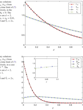
Example 1 First we consider the case:r =bandDr = Db, that is particles of the
same size and diffusivity. In this case, system (11) has a full gradient flow structure and hence we expect that the stationary states computed with the two approaches to be the same. We plot the two pairs,(r∗,b∗)computed as the long-time limit of (11), and(r∞,b∞), computed from (40) in Fig.1. The parameters are Dr = Db = 1,
r=b=0.01,Nb=Nr =200 andvr=2,vb=1. As expected, the solutions are
identical.
Example 2 From Corollary3.1, we expect the stationary solutions corresponding to
the case of an asymptotic and a full gradient flow equation agree up to orderO(d). To investigate this, we again compare the solutions(r∗,b∗)and(r∞,b∞)as we move away from the case with an exact gradient flow structure [which corresponds toθr= θb =0, see (21)–(23)]. We recall that the parametersθr andθbare only zero in the
Fig. 1 Stationary solutions
(r∗,b∗)and(r∞,b∞)from solving the long-time limit of (7) and (40), respectively, in the case withθr=θb=0. The
parameter values ared=2, Dr=Db=1,r=b=0.01,
Nb=Nr=200 andV˜r=2x,
˜ Vb=x
0 0.2 0.4 0.6 0.8 1
0 0.5 1 1.5 2
x
r∞
b∞
r∗
b∗
Fig. 2 Stationary solutions
(r∗,b∗)and(r∞,b∞)from solving the long-time limit of (7) and (40), respectively, in a case withθr=8·10−5. The
parameter values ared=2, Dr=0.2,Db=1, r=b=0.01,
Nb=Nr=200 andV˜r=2x,
˜ Vb=x
0 0.2 0.4 0.6 0.8 1
0 1 2 3 4 5 6 7 8 9
0 0.05 0.1
0 0.5 1 1.5 2
x x
r∞
br∞ ∗
b∗
a one-parameter sweep withθr, increasing it from 0 (as in Fig.1) to 9·10−5, while
keepingr=b=0.01 andDb=1 fixed. This ensures that whenθr=0 thenθb=0.
The reds diffusivityDris varied according to (23). We plot the result forθr=8·10−5
in Fig.2. As expected, the error between the stationary solutions is apparent.
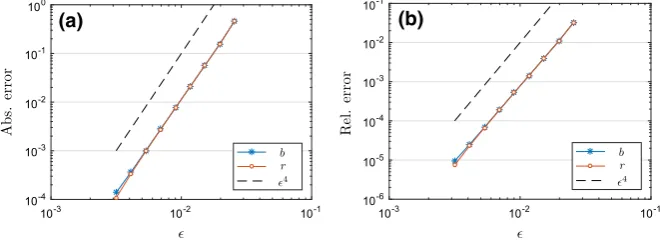
The absolute error and the relative error between the solutions, r∞−r∗ and
b∞−b∗andr∞−r∗/r∞andb∞−b∗/b∞, respectively, as a function ofθris shown in Fig.3.
To conclude this section, we compute the stationary solutions of the (exact) full system and that approximated by the asymptotic gradient flow system as we vary, where=b=r, while keeping all the other parameters fixed. We plot the results
[image:21.439.100.388.56.438.2]10-5 10-4 10-3
10-2 10-1 100
θr
b r
A
bs.
error
(a)
10-5 10-4
10-4 10-3 10-2 10-1
θr
b r
Rel.
er
ro
r
(b)
Fig. 3 Error between the stationary solution(r∗,b∗)of (7) and(r∞,b∞)of (40) as a function ofθr.a
Absolute error.bRelative error. Theredparticles diffusionDris varied according to (23), while the other
parameter values are fixed to:d=2,Db=1,r=b=0.01,Nb=Nr=200 andV˜r=2x,V˜b=x
10-3 10-2 10-1
10-4 10-3 10-2 10-1 100
b r
4
A
bs.
error
(a)
10-3 10-2 10-1
10-6 10-5 10-4 10-3 10-2 10-1
b r
4
R
el
.
error
(b)
Fig. 4 Error between the stationary solution(r∗,b∗)of (7) and(r∞,b∞)of (40) as a function of, where
=r=b.aAbsolute error.bRelative error. The parameter values are fixed to:d=2,Dr=2,Db=1,
Nb=Nr=200 andV˜r=2x,V˜b=x
5 Global Existence for the Full Gradient Flow System
In this section, we present a global in time existence result for the system with particles of same size and diffusivity (14). We look for a weak solution(r,b):×(0,T)→S
to the system
∂t
r b
= ∇ ·
Jr Jb
with
(1−γ ρ)Jr=(1−γ ρ) ((1− ¯γ ρ)∇r+(α¯+ ¯γ )r∇ρ+r∇Vr+ ¯γ∇(Vb−Vr)r b) (1−γ ρ)Jb=(1−γ ρ) ((1− ¯γ ρ)∇b+(α¯+ ¯γ )b∇ρ+b∇Vb+ ¯γ∇(Vb−Vr)r b) .
(41)
[image:22.439.57.385.55.180.2] [image:22.439.54.386.227.348.2]Theorem 5.1 (Global existence in the case of small volume fraction)Let T >0, let
(r0,b0): → S◦, whereS is defined by(25), be a measurable function such that
E(r0,b0) <∞. Then, there exists a weak solution(r,b):×(0,T)→Sto system
(41)satisfying
∂tr, ∂tb∈ L2(0,T;H1()), ρ ∈ L2(0,T;H1()),
(1− ¯γ ρ)2∇√r, (1− ¯γ ρ)2∇√b ∈L2(0,T;L2()).
Moreover, the solution satisfies the following entropy dissipation inequality:
dE
dt +D1≤C, (42)
where
D1=
2(1− ¯γ ρ)
4|∇√
r|2+2(1− ¯γ ρ)4|∇√b|2+γ¯
2|∇ρ|
2
dx
and C ≥0is a constant.
We recall that system (14) can be written as a gradient flow:
∂t
r b
= ∇ ·
M(r,b)∇
u v
, (43)
where
M =
r(1− ¯γb) γ¯r b
¯
γr b b(1− ¯γr)
.
Note that ifr,bandρ∈S◦, then the matrixMis positive definite.
We perform a time discretization of system (43) using the implicit Euler scheme. The resulting recursive sequence of elliptic problems is then regularized. LetN ∈N
and letτ =T/Nbe the time step size. We split the time interval into the subintervals
(0,T] = N
k=1
((k−1)τ,kτ], τ = T
N.
Then, for given functions(rk−1,bk−1)∈S, which approximate(r,b)at timeτ(k−1),
we want to find(rk,bk)∈Ssolving the regularized time discrete problem
1
τ
rk−rk−1
bk−bk−1
= ∇ ·
M(rk,bk)
∇ ˜uk
∇ ˜vk
+τ
u˜k− ˜uk vk˜ − ˜vk
where we use the modified entropy
˜
E =E+Eτ =
r(logr−1)+b(logb−1)+r Vr+bVb+ ¯
α
2
r2+2r b+b2
+τ(1− ¯γ ρ)(log(1− ¯γ ρ)−1)dx, (45)
with associated entropy variables
˜
u =u+uτ =logr+ ¯αρ+Vr−τγ¯log(1− ¯γ ρ),
˜
v=v+vτ =logb+ ¯αρ+Vb−τγ¯log(1− ¯γ ρ). (46)
The additional term in the entropy provides upper bounds on the solutions and the higher-order regularization terms guarantee coercivity of the elliptic system in
H1(), which is needed to show existence of weak solutions to a linearized version of the problem (44) using Lax–Milgram. The existence result of the corresponding nonlinear problem is concluded by applying Schauder fixed point theorem.
Finally, uniform a priori estimates inτ and the use of a generalized version of the Aubin–Lions lemma allow to pass to the limitτ →0 leading to the existence of (41). Note that the compactness results are sufficient for 1− ¯γ ρ >0 to pass to the correct limit in the flux termsJrandJb, i.e., leading to the global existence of weak solutions to system (14).
Lemma 5.1 The entropy density
˜
h:S◦→R,
r b
→r(logr−1)+b(logb−1)+r Vr+bVb
+α¯
2
r2+2r b+b2
+τ(1− ¯γ ρ)(log(1− ¯γ ρ)−1)
is strictly convex and belongs to C2(S◦).Its gradienth˜:S◦→R2is invertible and
the inverse of the Hessianh˜:S◦→R2×2is uniformly bounded.
Proof Note that
˜
h=
logr−τγ¯log(1− ¯γ ρ)+ ¯αρ+Vr
logb−τγ¯log(1− ¯γ ρ)+ ¯αρ+Vb
and
˜
h=
!1
r +τ γ¯ 2
1− ¯γ ρ + ¯α τ γ¯
2
1− ¯γ ρ + ¯α τ1− ¯γ¯γ ρ2 + ¯α
1 b+τ γ¯
2
1− ¯γ ρ + ¯α
"
.
The matrixh˜is positive definite on the setS◦, soh˜is strictly convex. We can easily deduce that the inverse ofh˜exists and is bounded onS◦.
Next, we verify the invertibility ofh˜. Note that the functiong=(g1,g2):S◦→
(x,y) ∈ R2 and define u(z) = (ex +ey)(1− ¯γz)for 0 < z < γ1¯. Then, u is nonincreasing and asu(0) > 0 andu
1 ¯
γ
= 0, there exists a unique fixed point 0 < z0 < γ1¯ such that u(z0) = z0. Then, we definer = ex(1− ¯γz0) > 0 and
b = ey(1− ¯γz0) > 0. It holds thatr+b = (ex +ey)(1− ¯γz0) = z0 < 1 ¯
γ. So,
(r,b)∈ S◦. Then, we define the function f = ˜h◦g−1 :R2 → R2. Sinceh˜ and
gare nonsingular matrices for(r,b)∈S◦, the Jacobian of f is also nonsingular for
(r,b)∈S◦. Furthermore, we have that
f(y)=y+χ(g−1(y)), y∈R2,
whereχ =
¯
αρ+Vr
¯
αρ+Vb
∈C0(S)⊆L∞(S◦). So,|f(y)| → ∞as|y| → ∞, which together with the invertibility of the matrixD f allow us to apply Hadamard’s global inverse theorem showing that f is invertible. So, alsoh˜is invertible.
5.1 Time Discretization and Regularization of System (43)
The weak formulation of system (44) is given by:
1
τ
rk−rk−1
bk−bk−1
· 1 2
dx+
∇1
∇2
T
M(rk,bk)
∇ ˜uk
∇ ˜vk
dx
+τR
1 2 , ˜ uk ˜ vk =0 (47)
for(1, 2)∈H1()×H1(), where(rk,bk)=h−1(u˜k,vk˜ )and
R 1 2 , ˜ uk ˜ vk =
1u˜k+2vk˜ + ∇1· ∇ ˜uk+ ∇2· ∇ ˜vkdxdy.
We defineF :S ⊆L2(,R2)→S ⊆L2(,R2), (r˜,b˜)→(r,b)=h−1(u˜,v)˜ , where(u˜,v)˜ is the unique solution inH1(,R2)to the linear problem
a((u˜,v), (˜ 1, 2))=F(1, 2) for all(1, 2)∈ H1(,R2) (48)
with
a((u˜,v), (˜ 1, 2))=
∇1
∇2
T
M(r˜,b˜)
∇u
∇v
dx+τR
1 2 , ˜ u ˜ v
F(1, 2)= −
1 τ ˜
r−rk−1
˜
b−bk−1