https://doi.org/10.5194/npg-26-91-2019
© Author(s) 2019. This work is distributed under the Creative Commons Attribution 4.0 License.
Statistical hypothesis testing in wavelet analysis: theoretical
developments and applications to Indian rainfall
Justin A. Schulte
Science Systems and Applications, Inc., Lanham, Maryland 20706, USA Correspondence:Justin A. Schulte ([email protected])
Received: 3 December 2018 – Discussion started: 13 December 2018 Revised: 1 May 2019 – Accepted: 2 May 2019 – Published: 14 June 2019
Abstract.Statistical hypothesis tests in wavelet analysis are methods that assess the degree to which a wavelet quantity (e.g., power and coherence) exceeds background noise. Com-monly, a point-wise approach is adopted in which a wavelet quantity at every point in a wavelet spectrum is individually compared to the critical level of the point-wise test. How-ever, because adjacent wavelet coefficients are correlated and wavelet spectra often contain many wavelet quantities, the point-wise test can produce many false positive results that occur in clusters or patches. To circumvent the point-wise test drawbacks, it is necessary to implement the recently developed area-wise, geometric, cumulative area-wise, and topological significance tests, which are reviewed and devel-oped in this paper. To improve the computational efficiency of the cumulative area-wise test, a simplified version of the testing procedure is created based on the idea that its out-put is the mean of individual estimates of statistical signif-icance calculated from the geometric test applied at a set of point-wise significance levels. Ideal examples are used to show that the geometric and cumulative area-wise tests are unable to differentiate wavelet spectral features arising from singularity-like structures from those associated with periodicities. A cumulative arc-wise test is therefore devel-oped to strictly test for periodicities by using normalized ar-clength, which is defined as the number of points compos-ing a cross section of a patch divided by the wavelet scale in question. A previously proposed topological significance test is formalized using persistent homology profiles (PHPs) measuring the number of patches and holes corresponding to the set of all point-wise significance values. Ideal exam-ples show that the PHPs can be used to distinguish time se-ries containing signal components from those that are purely noise. To demonstrate the practical uses of the existing and
newly developed statistical methodologies, a first compre-hensive wavelet analysis of Indian rainfall is also provided. An R software package has been written by the author to im-plement the various testing procedures.
1 Introduction
et al., 2007; Labat, 2010; Schulte et al., 2017), forecast model verification (Lane, 2007; Liu et al., 2011), ensemble forecast-ing (Schulte and Georgas, 2018), climate network analysis (Agarwal et al., 2018; Paluš, 2018; Ramana et al., 2013; Sa-hay and Srivastava, 2014; Elsanabary and Gan, 2004), and biomedicine (Addison, 2005).
One application of wavelet analysis is the estimation of a sample wavelet spectrum and the subsequent comparison of the sample wavelet spectrum to a background noise spec-trum. To make such comparisons, one must implement sta-tistical tests such as the point-wise (Torrence and Compo, 1998), area-wise (Maraun et al., 2007), geometric (Schulte et al., 2015), and cumulative area-wise (Schulte, 2016a) tests. Torrence and Compo (1998) were the first to place wavelet analysis in a statistical hypothesis testing framework using point-wise significance testing. In the point-wise approach, the statistical significance of wavelet quantities associated with points in a wavelet spectrum is assessed individually without considering the correlation structure among wavelet coefficients. For wavelet power spectra of climate time se-ries, theoretical red-noise spectra are often the noise back-ground spectra against which sample wavelet power spec-tra are tested. Monte Carlo methods are used to estimate the background noise spectra for wavelet coherence (Grinsted et al., 2004), partial coherence (Ng and Cha, 2012), multiple coherence (Hu and Si, 2016), and auto-bicoherence (Schulte, 2016b).
Despite its wide use, the point-wise approach has two drawbacks; the first of which is that the test will frequently generate many false positive results because of the simulta-neous testing of multiple hypotheses (Maraun et al., 2007; Schulte et al., 2015). The second drawback is that spuri-ous results occur in clusters because wavelet coefficients are correlated. To account for these deficiencies, Maraun et al. (2007) developed an area-wise test to reduce the num-ber of spurious results. Additional tests were subsequently developed by Schulte et al. (2015) and Schulte (2016a) to address the deficiencies of the point-wise test and compu-tational inefficiencies of the area-wise test. Although these tests were demonstrated as being effective in reducing spu-rious results, the point-wise testing procedure is still more frequently adopted. Furthermore, there are numerous papers surveying general aspects of wavelet analysis (Meyers et al., 1993; Kumar and Foufoula-Georgiou, 1997; Torrence and Compo, 1998; Labat, 2005, Lau and Weng, 1995; Addison, 2005; Schaefli et al., 2007; Sang et al., 2012) but no papers surveying the recent developments in statistical hypothesis testing. This observation underscores the need for a paper that summarizes theoretical and practical aspects of statisti-cal hypothesis testing.
A physical application to which wavelet methods have been applied is the understanding of Indian rainfall (Adarsh and Reddy, 2014; Maheswaran and Khosa, 2014). In-dian rainfall variability is a complex, non-stationary, and timescale-dependent phenomenon, making wavelet
analy-sis a well-suited tool for studying it. Recognizing the non-stationary behavior of the Indian monsoon phenomena, Tor-rence and Webster (1999) used wavelet coheTor-rence analysis to show that the relationship between the El Niño–Southern Oscillation (ENSO) and Indian rainfall is strong and non-stationary in the 2-year to 7-year period band. Narasimha and Bhattacharyya (2010) used wavelet cross-spectral anal-ysis to link the solar cycle to changes in the Indian mon-soon. Other studies have used wavelet analysis to understand the temporal characteristics of the Indian rainfall time series (Nayagam et al., 2009). Fasullo (2004) found biennial os-cillations in the all-India rainfall time series, while Yadava and Ramesh (2007) found significant long-term periodicities in an Indian rainfall proxy time series. Terray et al. (2003) found that a time series describing late summer (September– August) Indian rainfall is associated with significant wavelet power in the 2-year to 3-year period band and suggested that such power is related to the tropospheric biennial oscillation. Common to all the studies noted above is the use of point-wise significance testing. Recent work highlighting the pit-falls of the point-wise testing approach raises the question as to whether the features identified in previous wavelet studies of Indian rainfall are statistical artifacts or ones distinguish-able from the background noise. To address this question, an additional study is needed that applies the new statistical hy-pothesis tests in wavelet analysis.
In this paper, a first review of the theoretical and practi-cal aspects of recent advances in statistipracti-cal significance test-ing of wavelet estimators is presented in Sect. 2. Section 2 also includes discussions about the modifications of existing tests designed to make them more computationally efficient than the original formulations. A cumulative arc-wise test is also proposed for testing for the presence of periodicities em-bedded in noise in a strict sense. Section 3 is devoted to the presentation of a comprehensive wavelet analysis of Indian rainfall time series using recently developed wavelet meth-ods. The paper concludes with a summary and discussion in Sect. 4.
2 Wavelet analysis 2.1 Basic overview
The continuous wavelet transform of a time seriesX(t ) is given by
W (b, a)= √1
a Z ∞
−∞ X(t )ψ∗
t−b
a
dt, (1)
re-ferred to as the timescale plane. To simplify the discussion of results in this paper, the commonly used Morlet wavelet with angular frequencyω=6 is used throughout. For more details about wavelet analysis, the reader is referred to Torrence and Compo (1998).
Unlike the Fourier analysis where neighboring frequen-cies are uncorrelated, the wavelet coefficients at neighboring points inH are intrinsically correlated. The intrinsic corre-lation between wavelet coefficients at (b,a) and (b0, a0) is represented by the reproducing kernelK(b, a,b0,a0) whose mathematical expression is
K b, a;b0, a0= 1 cψ
√ aa0
Z ψ
t−b0
a0
ψ∗
t−b a
dt, (2) wherecψ is an admissibility constant. The redundancy
be-tween the valuesW (a, b)andW a0, b0
is expressed as W (b, a)=
Z Z
K b, a;b0, a0
W a0, b0da 0
a02db
0
. (3)
Equation (3) says that a wavelet coefficient atW (b, a) cap-tures information from neighboring points; the degree to which this occurs depends on the weight K b, a;b0, a0. Even for uncorrelated noise, wavelet coefficients will be cor-related inH (Maraun and Kurths, 2004), a theoretical result that has important implications for significance testing.
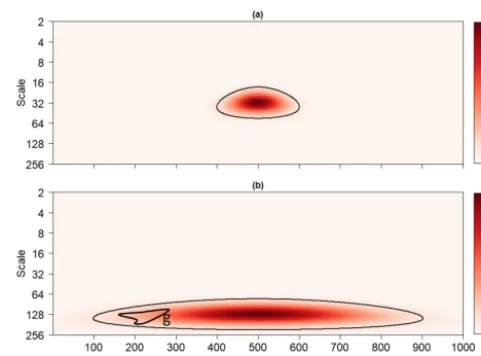
The normalized reproducing kernel for the Morlet wavelet is shown in Fig. 1, where normalization means that the re-producing kernel is divided by its maximum value so that the maximum of the normalized reproducing kernel is equal to unity and located at the point at which the reproducing ker-nel is centered. In Fig. 1a, the reproducing kerker-nel is dilated and translated to the scalea=32 and timeb=500 and indi-cates that a wavelet coefficient at (500, 32) will be correlated with other wavelet coefficients surrounding it. The reproduc-ing kernel shown in Fig. 1b is dilated and translated to (500, 128) and seen as being wider in the time direction than the reproducing kernel centered at (500, 32). The widening re-flects how the reproducing kernel expands linearly in both the time and scale (in a non-logarithmic scale) direction. 2.2 Statistical significance tests
2.2.1 Point-wise significance
In point-wise significance testing, one individually compares a wavelet quantity at every point inHto the critical level of the point-wise test, which depends on the chosen point-wise significance levelαpwand usually on the wavelet scalea. For
wavelet power spectra of climate time series, point-wise test critical values are often determined from a theoretical red-noise background (Torrence and Comp, 1998). For wavelet coherence, partial coherence, multiple coherence, and auto-bicoherence, Monte Carlo methods need to be implemented to estimate the critical values (Grinsted et al., 2004; Ng and Chan, 2012; Hu and Si, 2016; Schulte, 2016b). However, a
Figure 1.The normalized reproducing kernel of the Morlet wavelet dilated and translated to(a)(500, 32) and(b)(500, 128). Contours enclose the regions in the timescale plane where the normalized re-producing kernel exceeds 0.1. The closed pathgin Fig. 1b can be continuously deformed into a point so that it does not surround a hole in the contoured region.
parametric bootstrap method may be required for determin-ing the critical values of an arbitrary background model if analytical background models are not readily available (Ma-raun et al., 2007). Using the point-wise test, one assigns to each point inH ap value,ρpw, representing the
probabil-ity of finding the observed or more extreme wavelet quantprobabil-ity (power, coherence, etc.) when the null hypothesis is true. The result of the point-wise test is the subset
Ppw=
(b, a):ρpw(b, a) < αpw , (4)
of H, representing regions where point-wise significant wavelet quantities have been identified.
To better understand the utility of the point-wise testing procedure, consider two example time series, where the first time series,R(t ), corresponds to a realization of a red-noise process with a lag-1 autocorrelation coefficient equal to 0.4 (Fig. 2a). The second time series,X(t ), shown in Fig. 3a, is given as
X (t )=S (t ) /σs+N (t )/mσn, (5)
where
S (t )=
3
X
j=1
sin 2π
2j+5t+δ(t ), (6)
δ (t )=
60 t=1000
0 otherwise, (7)
andN (t )is a realization of a red-noise process with a lag-1 autocorrelation coefficient equal to 0.1. The constantsσsand
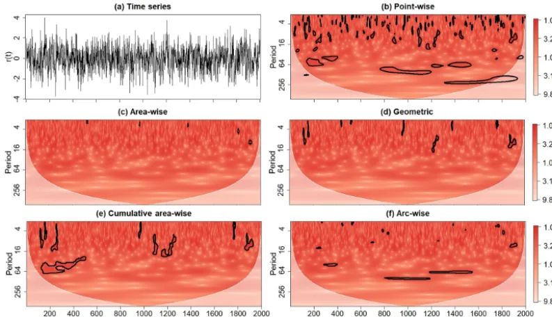
Figure 2. (a)A realization of a red-noise process (denoted byR(t ))with lag-1 autocorrelation coefficient equal to 0.4 together with its rectified wavelet power spectrum after the application of the (b)point-wise,(c)area-wise,(d)geometric,(e)cumulative area-wise, and
(f)cumulative arc-wise tests. The point-wise, cumulative arc-wise, and cumulative area-wise tests were applied at the 5 % significance levels. The geometric and area-wise tests were applied at the 0.01 level to 5 % point-wise significance regions. Contours enclose regions of statistical significance. Light shaded region represents the cone of influence where edge effects become important.
The real numbermis a measure of the signal-to-noise ratio, with larger values indicating a relatively higher signal.
The outcomes of the point-wise test applied to the (recti-fied; Liu et al., 2007) wavelet power spectrum ofX(t )and R(t )are shown in Figs. 2b and 3b. ForR(t ), the point-wise test applied at αpw=0.05 identified many statistically
sig-nificant wavelet power coefficients, all of which being spuri-ous by construction. The spurispuri-ous results are seen occurring in contiguous regions, and the union of all such regions is Ppw. For the wavelet power spectrum ofX(t ), statistically
significant wavelet power at the periods 64, 128, and 256 is seen clustering in narrow bands, reflecting the periods of the individual sinusoids (Fig. 3b). The singularity at t=1000 emerges as a scale-elongated region of point-wise signifi-cance, extending from a period of 2 to a period of approx-imately 32. What about the other features seen in the wavelet power spectrum? All the other significance regions are spu-rious by construction because they are associated with the noise term N (t ), implying that they resulted from stochas-tic fluctuations. Thus, without further investigation, it would be impossible to know without prior knowledge of X(t )if the features associated with N (t ) are part of the signal or not. These examples highlight how the number of spurious results can be large and how they could impede the differen-tiation between an underlying signal and background noise. It is therefore important to reduce the number of spurious results using other statistical methods.
2.2.2 Area-wise and geometric testing
As noted by Maraun et al. (2007), the application of the point-wise testNpw times will on average produceNpwαpw
spurious results, with the spurious results occurring in clus-ters or patches. These so-called point-wise significance patches arise from the reproducing kernel of the analyzing wavelet that represents intrinsic correlations among wavelet coefficients. As noted by Schulte (2016a), patches can be rig-orously defined using ideas from topology. That is, a patch is a path-connected component ofPpw, where a path-connected
component is an equivalent class ofPpw resulting from an
equivalence relation∼onPpwthat makes pointsx, y ∈Ppw
equivalent (writtenx∼y)if they can be connected by a con-tinuous pathf:[0 1]→Ppwsuch thatf (0)=xandf (1)=
y (Fig. 4). The equivalence relation∼reduces the original large set of points inPpwto a smaller set of patches; the
im-plications of which will be described later.
sug-Figure 3.Same as Fig. 2, except for the ideal time seriesX(t )representing the linear superposition of three sinusoids with period equal 64, 128, and 256; a singularity att=1000; and a realization of red-noise process with lag-1 autocorrelation coefficient equal to 0.1. The signal-to-noise ratio,m, is equal to 0.4.
Figure 4.Four point-wise significance patches whose union is the set of all point-wise significant values. The closed pathgencircles a hole, while the pathf connects the pointsxandybelonging to the same path component or patch. The patch containing the points zandwis convex, contrasting with the patch containing the points pandq.
gests that typical patches will be convex, which can be con-firmed by generating a large ensemble of patches found in the wavelet power spectra of realizations of a red-noise pro-cess (Schulte et al., 2015). The convexity of patches plays an important role in understanding how different statistical tests perform. Another important geometric property is area, which reflects the dilated reproducing kernel so that patches at greater scales will be generally larger than those located at smaller scales, as Fig. 1 suggests.
Recognizing that a typical patch area is given by the repro-ducing kernel, Maraun et al. (2007) developed an area-wise test, which is conducted as follows. First choose a critical area Pcrit(b, a)defined as a subset ofH for which the
re-producing kernel dilated and translated to (b,a)exceeds a
certain critical levelKcrit. That is,
Pcrit(b, a)=
b0, a0|K b, a;b0, a0> Kcrit . (8)
The set of points whose associated wavelet quantities are also area-wise significant is then the set
Paw=
[
Pcrit(b,a)⊂Ppw
Pcrit(b, a) , (9)
representing the union of all critical areas that lay completely insidePpw. The larger the critical area, the larger a patch
needs to be for it to be deemed area-wise significant so that Pcrit(b, a)is related toαaw, the significance level of the
area-wise test. As discussed by Maraun et al. (2007), the criti-cal area that corresponds toαaw is determined using a
root-finding algorithm, which is a non-trivial step that can be cir-cumvented by performing a geometric test instead, as dis-cussed below.
While the area-wise test effectively addresses the multiple-testing pitfall of the point-wise test, the use of the root-finding algorithm renders the practical implementation of the test difficult. To overcome this drawback, Schulte et al. (2015) constructed a geometric test whose test statistic is normalized area, which is defined as the patch area,Apatch,
divided by the square of the patch’s mean scale coordinate,
ˆ
a. That is,
Anorm=
Apatch
ˆ
a2 , (10)
expansion of patches in the time and scale direction. Thus, the normalized areas of patches can be readily compared re-gardless of where the patches are in H. The critical value of this test is assessed using Monte Carlo methods as fol-lows: (1) generate wavelet spectra under some null hypoth-esis (e.g., red noise), (2) create a null distribution of nor-malized area using the patches found in the wavelet spectra, and (3) estimate the critical level of the test corresponding to the geometric significance level αgeo by computing the
percentile of the null distribution corresponding to 1-αgeo.
This null distribution calculation can be performed rapidly because wavelet spectra often contain many patches. How-ever, for wavelet coherence, Monte Carlo methods must be applied twice because the critical levels of the point-wise test must be also empirically estimated. Fortunately, the length of the noise realizations needed to generate the null distribution of normalized areas need not be the same length of the input time series because the patch area is unrelated to the time se-ries length; it is related to the reproducing kernel. As such, the realizations can be of shorter length, improving the ef-ficiency of the null distribution computation. The ability to efficiently generate a null distribution allowspvalues asso-ciated with the geometric test to be further adjusted to ac-count for multiple testing. For example, the false discovery rate of the geometric test can be controlled at a desired level if the number of patches to which the test is applied is large (Schulte et al., 2015).
It is important to note that the geometric and area-wise tests differ in the way they assign statistical significance to points. For the geometric test, all points in a patch will be deemed insignificant or significant if the patch is deemed sta-tistically insignificant or significant. However, strictly speak-ing, the area-wise test evaluates the statistical significance of wavelet quantities associated with points inPpwbased on the
geometric properties of the path-connected subsets of Ppw
to which they belong. That is, for a wavelet quantity at (b, a) to be area-wise significant means that there must be a P ⊆Ppwcontaining (b,a) that is path-connected, sufficiently
convex, and large enough to havePcrit(b, a)⊂P. IfP is a
patch, then no subset ofP can be area-wise significant ifP is not, consistent with the patch-sorting interpretation. On the other hand,P may contain both area-wise and non-area-wise significant subsets, opposing the patch-sorting interpretation. As discussed earlier, the equivalent relation ∼reduces the initial large set of points to a set of fewer patches, implying that the number of spurious results arising from the geomet-ric and area-wise test is less than that of the point-wise test.
Figures 2 and 3 show the wavelet power spectra ofX(t ) andR(t )after the application of the area-wise and geomet-ric tests at the 0.1 significance level, where the area-wise test was performed using an existing R software package (available at https://rdrr.io/github/Dasonk/SOWAS/, last ac-cess: 12 January 2018). Both tests are seen reducing the number of spurious results arising from the point-wise sig-nificance test applied at the αpw=0.05 level. However, as
shown in Fig. 3c, the area-wise test also deems features asso-ciated with the signalS(t )to be noise. For example, the patch located at a period of 256 extending fromt=100 tot=1700 is no longer statistically significant. Note also that the area-wise test largely filters out the scale-elongated feature asso-ciated with the singularity ofX(t )att=1000, while the ge-ometric test deems the feature to be statistically significant. This difference in performance is expected because patches must be long with respect to the reproducing kernel to be area-wise significant, whereas there is no such constraint for the geometric test. Thus, the area-wise test is better suited for situations in which only periodicities are sought because periodicities induce temporally long patches. In general, the area-wise and geometric tests will reduce the signal detected by the point-wise test because the area-wise and geometric tests are theoretically constrained to detect a smaller amount of signal than the point-wise test (Table A1). This theoretical constraint raises a natural question: can a test simultaneously reduce statistical artifacts and increase signal detection (true positive results) relative to the point-wise test? The fact that patches enlarge with increasingαpwsuggests that examining
the areas of patches across a set of point-wise significance levels could improve signal detection relative to the point-wise test.
2.2.3 Cumulative area-wise testing
Maraun et al. (2007) and Schulte et al. (2015) demonstrated that the area-wise and geometric tests are procedures for re-ducing the number of spurious results. However, both tests suffer from the drawback of having to select both an area-wise (or geometric) significance level and a point-area-wise sig-nificance level. This dual sigsig-nificance level selection is a cause for concern because a single wavelet quantity can have different levels of area-wise or geometric significance de-pending on the chosen point-wise significance level, leading to uncertainty as to whether the wavelet quantity is statisti-cally artificial or distinguishable from background noise.
To address this concern, Schulte (2016a) suggested that changes in the geometric and topological characteristics of patches should be assessed over a finite set of point-wise sig-nificance levelsα1, α2, . . ., αN. If the point-wise significance
levelsα1, α2, . . ., αN are chosen such that
α1< α2< . . . < αN, (11)
then the sets Ppwi =
(b, a):ρpw(b, a) < αi , (12)
will form a filtration
∅=Ppw1 ⊆P 2
pw⊆. . .⊆P
N
pw=H, (13)
ofH for a sufficiently smallα1and large αN value.
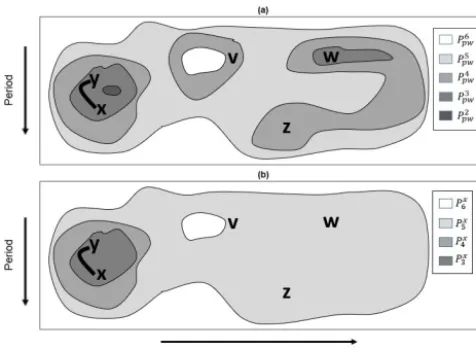
Figure 5. (a)An idealized example of a timescale plane filtration and(b)a geometric pathway corresponding to the pointxand the filtration shown in(a). The first two members of the geometric path-way shown in(a)are the empty set and are not shown.
build the complete timescale plane by increasing the point-wise significance level to a value that renders all wavelet quantities statistically significant.
An idealized example of a wavelet domain filtration is shown in Fig. 5a. The application of the point-wise test at the α1level results in no statistically significant regions, whereas
the application of the test atα2results in a relatively small
re-gion of point-wise significance (dark gray). In contrast, set-ting the point-wise significance level toα5results in nearly
all wavelet quantities being statistically significant, as indi-cated by the light gray region. At α6, all wavelet quantities
are statistically significant, andPpw6 isH.
Although filtrations like Eq. (13) have proven to be useful in a data analysis method called persistent homology (Edels-brunner and Harer, 2008), this method focuses on the sets of all point-wise significant values. At present, the concern is the statistical significance of a wavelet quantity at a point, and thus a more local approach is needed, though the util-ity of Eq. (13) will become more apparent in Sect. 2.2.5. To localize the persistence approach, a local filtration about x called a geometric pathway is needed (Schulte, 2016a). Mathematically, a geometric pathway Gx corresponding to
a pointxis a nested sequence
∅=P1x⊆P
x
2 ⊆. . .⊆P
x
N=H, (14)
where Pix= n
(b, a):(b, a)∈Ppwi , (b, a)∼x o
. (15)
A concrete example of a geometric pathway Gx is shown
in Fig. 5b, where the geometric pathway corresponds to the wavelet domain filtration shown in Fig. 5a. In this exam-ple, P1x=∅andP2x=∅, where P2x=∅becausex is not in the dark gray region shown in Fig. 5a representingPpw2 .
Although the set Ppw3 comprises two path components or patches, only the component containing bothx andy corre-sponds to the geometric pathway member atα3. The reason
is because any point equivalent towis not equivalent toxon Ppw3 , as those points cannot be connected toxby a path fully contained inPpw3 . Thus, in this example,
P3x=n(b, a):(b, a)∈Ppw3 and(b, a)∼xo, (16) y∈P3x, andw6∈P3x. A similar situation occurs at α4
be-causePpw4 has three path-connected components containing v, w, x, y, and z, but x is only equivalent to points that are equivalent to y. At α5, the set Ppw5 is path-connected
(x∼y∼z∼v∼w) and is thus the fifth member ofGx. The
sixth and last member ofGxisH.
Using the definition of a geometric pathway, Schulte (2016a) constructed a cumulative area-wise test that assesses the statistical significance of wavelet quantities by associating, to each point x in H, the total normalized area integrated over its geometric pathwayGx.
The first step of the procedure is to calculate the normalized areasAx1, Ax2, . . ., AxN corresponding to the N members of Gx, whereAxi is assumed to be zero ifPix=∅orPix= {x}.
The second step is to compute the sum,
Ax= N
X
k=1
Axk, (17)
and compareAxto a critical areaAcritdetermined by Monte
Carlo methods. In the Monte Carlo approach, wavelet spec-tra and corresponding geometric pathways are generated un-der some null hypothesis, and a null distribution is calcu-lated from all the computed total normalized areas. The crit-ical area corresponding to theαc level of the test is the
per-centile of the null distribution corresponding to 1-αc.
Per-forming these steps for all x∈H results in an adjustedp value at every point that accounts for multiple testing and the correlation among adjacent wavelet coefficients. As noted by Schulte (2016a), the computational efficiency of the cumula-tive area-wise test can be improved by settingα1=0.02 and
αN=0.18, though this selection means that the cumulative
area-wise test may no longer adjustpvalues at every point in H because complete filtrations like Eq. (13) may no longer be under consideration. Nevertheless, using a limited range of point-wise significance levels generally results in a better performance of the cumulative area-wise test relative to the geometric test performed at a single point-wise significance level (Appendix A and Table A1).
The criterion for a point to be cumulative area-wise signifi-cant is then
ˆ
Ax= 1
N
N
X
k=1
Axk >AˆCrit, (18)
whereAˆCritis the critical level of the test calculated by
com-puting the percentile of the null distribution comprising mean normalized areas corresponding to 1−αc. Furthermore, there
is a one-to-one relationship between the normalized area of a patch and its geometric testpvalue because a greater nor-malized area always means a lowerpvalue. Thus, ifρxi is the p value associated withAxi, then the criterion for a wavelet quantity to be cumulative area-wise significant is
ˆ
ρx= 1
N
N
X
k=1
ρkx< αc, (19)
because there is also a one-to-one relationship between αc
and the critical level of the test. Equation (19) implies that to perform the cumulative area-wise test, one can individ-ually perform the geometric test at each point-wise signifi-cance level and then computeρˆx, avoiding the computation of nested sequences as in the original formulation of the cu-mulative area-wise test.
This interpretation of the cumulative area-wise test also al-lows the testing method to be put in an ensemble forecasting framework. That is, the individual geometric test p values are identified as ensemble members estimating the statisti-cal significance of a wavelet quantity. The mean pvalue is identified with the ensemble mean that smooths out the un-predictable aspects of the forecast. In the present context,ρˆx
smooths out the features in the wavelet spectra resulting from noise and leaves the features that most of the geometric tests agree to be significant. This smoothing results in the sup-pression of noise but enhancement of the signal, which is consistent with how Schulte (2016a) found the cumulative area-wise test to perform superiorly to the geometric test in terms of signal detection, at least for periodic signals (Ap-pendix A and Table A1).
Using Eq. (19), we now devise a simplified approach to the cumulative area-wise test. In the simplified approach, all points in H are initially assigned a value of 0. Then, for a fixed point-wise significance level, the geometric test is per-formed on all patches. The points falling in those patches that are geometrically significant at theαclevel are then assigned
the value 2. The values for the points not in geometrically significant patches are left unchanged. This assignment step is then repeated for each point-wise significance level, and the values are stored separately so that each point in H is assigned a set of values, the number of values equaling the number of point-wise significance levels used to implement the cumulative area-wise test. Then, the average value at each point is computed, with regions where the average value ex-ceeds unity deemed to be cumulative area-wise significant.
The application of the simplified cumulative area-wise test to the wavelet power spectra of R(t ) and X(t ) (Figs. 2e and 3e) reveals that the test is effective at reducing the num-ber of spurious results arising from the point-wise test when applied at the αc=0.05 level. Like the area-wise test, the
reduction in spurious features is accompanied by a loss in signal detection. For example, the cumulative area-wise test, like the area-wise test, deems the wavelet power associated with the point-wise patch located at a period of 256 extend-ing fromt=100 tot=1700 in Fig. 3b to be statistically in-significant. On the other hand, the scale-elongated feature as-sociated with the singularity ofX(t )att=1000 more clearly emerges from the application of the cumulative area-wise test than the area-wise test, which is not surprising because the cumulative area-wise test assesses statistical significance based on area without regard to the specific shape of patches. Although this example suggests that the point-wise test de-tects a higher amount of signal than the cumulative area-wise test, a simplified experiment in Appendix A revealed that the simplified cumulative area-wise test can detect a higher amount of signal than the point-wise test when the signal-to-noise ratio is relatively high (Table A1). At low point-wise significance levels, the tests were found to detect a similar amount of the signal on average. Thus, a key strength of the cumulative area-wise test is that it can retain the signal while also reducing the number of spurious results arising from the point-wise test.
2.2.4 Cumulative arc-wise testing
While the area-wise, geometric, and cumulative area-wise tests can effectively reduce the number of spurious results, they do not test for the existence of periodicities embedded in a time series. This deficiency is especially true for the geometric and cumulative area-wise tests because they only consider the area of patches in the assessment of statistical significance. For example, the cumulative area-wise test can identify features that are long in scale but short in time as statistically significant (Fig. 3e). Thus, a new test needs to be constructed that is specifically designed to distinguish ran-domly stable fluctuations from those that are periodicities. As periodicities are determined by patch length, a strict test for periodicities should consider patch length and not patch area.
procedure for a finite set of point-wise significance levels al-lows for the assignment of total arclength to each point in the timescale plane. The null distribution can be computed using the Monte Carlo approach adopted for the cumulative area-wise test.
The application of the cumulative arc-wise test at the 0.05 significance level to the wavelet power spectra of X(t )and R(t )is shown in Figs. 2f and 3f, where point-wise signifi-cance levels ranging from 0.02 to 0.18 were used. The dis-crete spacing between adjacent point-wise significance was set to 0.02 to be consistent with the cumulative area-wise test applied earlier (Figs. 2e and 3e). Like with the other sta-tistical tests, the number of spurious point-wise test results for both time series is seen as being dramatically reduced. ForX(t ), much of the signal detected by the point-wise test remains despite the greater stringency of the cumulative arc-wise test. A comparison of Fig. 3c and f reveals that the geo-metric and cumulative arc-wise tests detect a similar amount of the signal associated with the three sinusoids. As expected, the cumulative arc-wise test, like the area-wise test, largely filters out the scale-elongated feature shown in Fig. 3b, sup-porting the idea that both the arc-wise and area-wise tests should be preferred to the geometric and cumulative area-wise tests in situations in which features associated with pe-riodic signals are sought. In fact, in Appendix A it is shown that the cumulative arc-wise test can detect a higher amount of signal than the point-wise test for high signal-to-noise ra-tios.
2.2.5 Topological significance testing
A common theme among all the statistical procedures dis-cussed so far is that they evaluate the statistical significance of wavelet quantities based on the geometric properties of the patches to which the corresponding points belong. How-ever, as demonstrated by Schulte et al. (2015), topological properties are also important to statistical hypothesis testing. How do topological properties differ from geometric ones? Topological properties of an object are those that remain un-changed no matter how much the object is twisted or bent. Using topological characteristics of point-wise significance regions, additional information about the time series in ques-tion can be gained.
The basic principal behind topological significance test-ing is that topologically equivalent (that is, homeomorphic) objects have identical topological invariants (Ferri, 2017). In the present context, the object of interest isPpwand the
topo-logical invariants of concern are the 0- and 1-D Betti num-bers denoted by β0 andβ1, respectively. The invariant β0
measures the number of path components or patches com-posingPpw, whereasβ1measures the number of 1-D holes
inPpw. A region inPpw has a hole if there is a closed path
in it such that the path cannot be continuously deformed into a point (Fig. 4). Equivalently, holes are regions in H fully surrounded by points in Ppw. Although counter-intuitive,
Schulte et al. (2015) showed that the presence of these holes is related to the statistical significance of the patch to which they correspond. To better understand how these holes are related to statistical significance, consider the reproducing kernel shown in Fig. 1b together with the set of points en-closed by the black contour. As shown in Fig. 1b, the en-closed path, g, in the contoured region can be continuously (e.g., no tearing or cutting) deformed into a point within the set by contracting or shrinking it, with this property holding for any closed path so that the set enclosed by the contour has no holes. As patches arise from the reproducing kernel, typi-cal patches arising from isolated fluctuations will tend not to have holes at low point-wise significance levels. However, if two fluctuations are located at nearby frequencies and times, then the resulting patches in the wavelet power spectrum may contain holes (Schulte et al., 2015).
Using Betti numbers, one can assess whetherPpwis
home-omorphic to Pnoise=(b, a):ρnoise(b, a) < αpw , where
ρnoisedenotes thep value resulting from the application of
the point-wise test to a noise spectrum such as the wavelet power spectrum associated with a realization of a red-noise process or the coherence spectrum associated with a pair of red-noise realizations. More specifically, a topological sig-nificance test is performed as follows: (1) compute wavelet spectra under some noise model, (2) computePnoisefor each
of the wavelet spectra, and (3) compute the null distribution of β0 andβ1. The critical values associated with the
two-sided topological significance test applied at theαtopo
signif-icance level are the percentiles of the null distribution cor-responding to 1-αtopo/2 andαtopo/2. The two-sided test
ac-counts for how the number of patches or holes can be un-usually high or low relative to noise. However, as shown by Schulte et al. (2015), a typical patch found in the wavelet power spectrum of red noise will typically have no holes at point-wise significance levels less than 0.2, suggesting that a one-sided topological test may be better than a two-sided test at low point-wise significance levels.
Topological equivalence at a single point-wise significance does not necessarily mean that the time series in question is topological indistinguishable from background noise. That is, the result of the topological significance test may be sen-sitive to the chosen point-wise significance level. To address this concern, it is necessary to adopt the persistent homol-ogy approach (Edelsbrunner and Harer, 2008) in which a topological space is distinguished from another topological space homeomorphic to it through an examination of filtered versions of the spaces (Ferri, 2017). In the wavelet analysis context, the spaces are the timescale planes associated with noise and the times series in question, which are rectangu-lar and topological equivalent. To distinguish the timescale planes, it is necessary to examine the filtered versions of the timescale planes using the filtration represented by Eq. (13). Computing βo and β1 at each step in the filtration results
Figure 6. (a) The 1-D and(b) 0-D persistent homology profiles associated with R(t ) and X(t ). Gray shaded region is the non-rejection region of the topological significance test applied at the 0.05 significance level. The non-rejection region was calculated by generating 100 realizations of a red-noise process with lag-1 auto-correlation equal to 0.1, the lag-1 autoauto-correlation coefficient corre-sponding toX(t ).
then involves comparing PHPs for a time series in question to that of noise by applying the topological significance test at each point-wise significance level.
The utility of the topological significance testing proce-dure is demonstrated using the wavelet power spectra ofX(t ) and R(t ). The 1-D PHP corresponding to R(t ), shown in Fig. 6a, indicates thatβ1is maximum atαpw=0.7 and
de-creases rapidly until reaching 0 at αpw=0.1. The overall
curve is the same for realizations of a red-noise process with any lag-1 autocorrelation coefficient, though the number of holes is greater for larger lag-1 autocorrelation coefficients (not shown). The 1-D PHP forX(t )is like that ofR(t ), sug-gesting that these time series are topologically indistinguish-able. The application of the topological significance test with αtopo=0.05 further supports the topological equivalence of
X(t )with red noise because the PHP associated withX(t ) falls in the gray-shaded envelope representing the test non-rejection region, where the non-non-rejection region was obtained by generating 100 PHPs associated with 100 realizations of a red-noise process with a lag-1 autocorrelation coefficient equal to that of X(t ). However, X(t )is not noise by con-struction, and thus the similarity of 1-D PHPs does not ex-clude the possibility that time series under consideration are indistinguishable from noise.
In contrast to the 1-D PHPs, the 0-D PHPs for X(t )and R(t )differ substantially (Fig. 6b). The PHP forX(t )is seen to reach a global maximum aroundαpw=0.25, while the one
for R(t ) peaks aroundαpw=0.18. The application of the
topological significance test at the 0.05 level strongly sup-ports the idea thatX(t )is distinguishable from noise because β0 far exceeds the critical level of the test atαpw=0.25.
Thus, there are features that are distinguishable from the background noise. These features are precisely those identi-fied from the area-wise, geometric, cumulative arc-wise, and cumulative area-wise tests.
3 Practical applications to the Indian monsoon 3.1 Data
To understand the temporal behavior and spatial variability of Indian rainfall, monthly rainfall data for five homogenous re-gions (Parthasarathy et al., 1994) extracted from Indian Insti-tute of Tropical Meteorology website (https://www.tropmet. res.in/DataArchival-51-Page, last access: 15 March 2019) were analyzed. The five divisions called the Peninsula, Northwest, Northeast, Central Northeast, and West Central regions were devised based on continuity of area, contribu-tion to annual amount, and global and regional circulacontribu-tion parameters (Parthasarathy et al., 1994; Azad et al., 2010). The rainfall data for each region were obtained by area-weighted averaging the sub-divisional data corresponding to the meteorological subdivisions composing the homogenous region, where the sub-divisional data were obtained by aver-aging the rainfall data associated with representative rainfall gauges. An all-India (Parthasarathy et al., 1995) rainfall time series was also examined, as it is commonly reported in the literature. The monthly all-India rainfall time series is con-structed by averaging the sub-divisional data after assigning a weight to each sub-division, which is determined by the sub-divisional area (Parthasarathy et al., 1994). These rain-fall data span the long time period from 1871 to 2016 and are continuous, making them well-suited for a wavelet analysis. Each rainfall time series was converted into an anomaly time series by subtracting the 1871–2016 mean for each month from the individual monthly values. After the conversion to an anomaly time series, the time series were standardized by dividing them by their respective 1871–2016 standard devia-tions. The resulting time series are shown in Fig. 7.
The monthly Niño 3.4 index (available at https://www.esrl. noaa.gov/psd/gcos_wgsp/Timeseries/Data/nino34.long.data, last access: 15 March 2019) from 1871 to 2016 was used to characterize the state of the ENSO system. The Niño 3.4 index is defined as the average SST in the region bounded by 5◦N and 5◦S and by 170 and 120◦W. The seasonal cycle was removed from this time series in the same way as it was removed from the rainfall time series.
3.2 Wavelet power spectrum
The wavelet power spectra corresponding to the rainfall time series are shown in Fig. 8, whereαpw=0.05 in this case.
se-Figure 7.Standardized(a)all-India,(b)Peninsula,(c)Northwest,(d)Northeast,(e)Central Northeast, and(f)West Central rainfall time series.
Figure 8.Wavelet power spectra of the standardized(a)all-India,(b)Peninsula,(c)Northwest,(d)Northeast,(e)Central Northeast, and
(f)West Central rainfall time series after the application of the point-wise test at the 0.05 significance level. Contours enclose regions of statistical significance, and the light shaded region represents the cone of influence where edge effects become important.
ries, with a large swath of point-wise significance being seen around a period of 256 months for the Peninsula, Northeast, and Northwest time series after 1950. For all the time se-ries, most of the point-wise significance patches are seen as being located at lower periods and appear to have varying geometries. For example, the wavelet power spectrum for the Northwest time series contains a scale-elongated significance patch at around 1920, extending from a period of 4 months to a period of 64 months. A similar but less prominent
fea-ture is also evident in the wavelet power spectrum of all-India rainfall. For the remaining time series, no such features are readily identifiable from an inspection of the wavelet power spectra.
To account for how spurious results may result from mul-tiple testing, the cumulative area-wise test was applied at theαc=0.05 level to the wavelet power spectrum shown in
from 0.02 to 0.18, with the spacing between adjacent point-wise levels equaling 0.02. Like with the point-point-wise test, sta-tistically significant wavelet power is located around a period of 256 months for the Northwest and Northeast regions, rais-ing the possibility that these time series contain periodicities at that timescale (Fig. 9). For all the time series, most of the statistically significant results are seen at periods less than 64 months. Two of the most prominent features are the scale-elongated significance patches around 1920 in the all-India and Northwest wavelet power spectra. Because the wavelet power associated with these scale-elongated features remain statistically significant after the application of the cumula-tive area-wise, there is strong evidence that the correspond-ing fluctuations exceed the red-noise background.
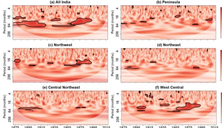
To better differentiate patches arising from singularities from those associated with periodicities, the cumulative arc-wise test was applied to wavelet power spectra shown in Fig. 8 at the same point-wise significance levels used for the cumulative area-wise test. As shown in Fig. 10, the ap-plication of the cumulative arc-wise test at the 5 % signifi-cance level reveals two time-elongated regions of statistical significance around a period of 256 months in the Peninsula and Northwest wavelet power spectra. However, the wavelet power around a period of 256 months is no longer statis-tically significant for the Northeast time series, suggesting that the point-wise significant wavelet power at that period is associated with a randomly stable oscillation. The scale-elongated features for the all-India and Northwest power spectra are largely filtered out like the scale-elongated fea-tures shown in Fig. 3 forX(t ). This result suggests that the wavelet power at that time and at those periods is associated with a singularity-like time domain feature rather than a pe-riodicity.
To gain a deeper understanding of the rainfall time ries, the 0th and 1-D PHPs were computed for each time se-ries. For clarity, we computed anomaly PHPs by subtracting the mean profile associated with noise from the individual profiles at each point-wise significance level. Thus, positive (negative) values mean that the number of patches (or holes) associated with the rainfall time series is greater (less) than that associated on average with noise. Because the lag-1 au-tocorrelation coefficients associated with each time series are nearly identical, a single test non-rejection region was com-puted using 100 realizations of a red-noise process with lag-1 autocorrelation coefficient equal to the mean lag-1 autocor-relation coefficient of the six rainfall time series. The mean noise profile was subtracted from both the upper and lower bounds of the test non-rejection region after the application of the topological significance test at the 0.05 level.
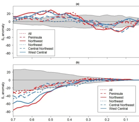
The 0th dimensional anomaly PHPs for each rainfall time series is shown in Fig. 11a. Many of the profiles are seen to deviate substantially from the mean noise profiles around αpw=0.5 andαpw=0.2. At aroundαpw=0.5, the largest
deviations are associated with the Northwest, West Central, and all-India time series. The profiles for the Northeast and
Peninsula time series lay inside the confidence envelope so that those time series could be topologically indistinguish-able from red noise. At aroundαpw=0.15, the largest
devi-ations are associated with the Northwest and Central North-east profiles. The large deviations from the mean noise pro-file for the Northwest time series suggest that the statisti-cally significant features identified by the cumulative area-wise test (Fig. 9) are unlikely statistical artifacts. On the other hand, the wavelet power spectrum of the West Cen-tral time series contains only five small regions of cumulative area-wise significance despite the large departures from the mean noise profiles at numerous point-wise significance lev-els. This finding raises the possibility of Type II errors for the cumulative area-wise test or a Type I error for the topological significance test.
Additional insight into the time series is provided by the 1-D anomaly PHPs shown in Fig. 11b. In this case, all the rainfall time series appear to be topologically distinguish-able from red noise for point-wise significance levels rang-ing from 0.7 to 0.65. Like with the 0th dimensional profiles, the departures are greatest for the Northwest and West Cen-tral time series, providing strong evidence that these time se-ries comprise features exceeding background noise. For the West Central time series, the lack of arc-wise significance shown in Fig. 10 suggests that the topological significance cannot be attributed to periodicities with high confidence. For the Northwest time series, the cumulative area-wise test re-sults suggest that topological significance may be attributed to the scale-elongated feature around 1915 and the enhanced wavelet power around a period of 256 months. The PHPs for all the time series converge to 0 below the point-wise sig-nificance level 0.3, and the lack of 1-D holes below 0.1 ren-ders the isolation of topologically significant regions in H using the approach of Schulte et al. (2015) that determines where there is enhanced topological significance based on the location of holes difficult. However, for the Northwest time series, a few holes were identified at point-wise signif-icance below 0.1 around the scale-elongated patches shown in Fig. 9c, supporting the results of the cumulative area-wise test.
3.3 Wavelet coherence
Figure 9.Same as Fig. 8 but after the application of the cumulative area-wise test at the 0.05 significance level.
Figure 10.Same as Fig. 8 but after the application of the cumulative arc-wise test at the 0.05 significance level.
The results for the wavelet coherence analysis are shown in Fig. 12. Statistically significant wavelet coherence was identified for all six time series, but coherence between the Niño 3. 4 index and the time series of rainfall is seen to be most salient for the all-India, Northwest, and West Central regions. The statistically significant coherence is mainly con-fined to the period band of 16 to 64 months, and time periods of enhanced coherence appear to follow time periods of weak coherence. The results shown in Fig. 12 suggest that the 16-month to 64-16-month mode of SST variability across the Niño 3.4 region modulates Indian rainfall, which is a well-known idea (Torrence and Webster, 1999). It is also noted that the coherence between rainfall and the Niño 3.4 index varies
spa-tially, consistent with recent work showing how ENSO influ-ences are spatially non-uniform (Roy et al., 2017).
4 Summary and discussion
Figure 11. (a)The 0-D and(b)1-D anomaly persistent homology profiles associated with the six rainfall time series. Gray shaded re-gion is the non-rejection rere-gion of the topological significance test applied at the 0.05 significance level. The non-rejection region was calculated by generating 100 realizations of a red-noise process with lag-1 autocorrelation equal to the mean of all six lag-1 autocorrela-tion coefficients associated with the rainfall time series.
timescale plane exceeds a background noise spectrum. This point-wise approach has been applied in numerous papers since its first application to wavelet analysis by Torrence and Compo (1998).
Despite its wide use, the point-wise test suffers from two pitfalls, as noted by Maraun and Kurths (2004) and Maraun et al. (2007) and as shown in Fig. 2. The first pitfall is that the test typically produces many false positive results because of the simultaneous testing of multiple hypotheses. Secondly, spurious results occur in clusters, with the clusters reflecting the reproducing kernel of the analyzing wavelet. To remedy the pitfalls of the point-wise test, Maraun et al. (2004) de-veloped an area-wise test to reduce the number of spurious point-wise significance patches based on the area and geom-etry of the patches. While the method has been shown to be effective at reducing the number of spurious results, the test is computationally inefficient. To address the concern of computational inefficiency, Schulte et al. (2015) proposed a geometric test that reduces the number of spurious results by assigning a normalized area to each patch. However, both the area-wise and geometric test suffer from a binary deci-sion pitfall in which both an area-wise (or geometric) sig-nificance level and a point-wise sigsig-nificance level must be selected. This dual selection inevitably leads to uncertainty regarding the statistical significance of a wavelet quantity.
Schulte (2016a) developed a cumulative area-wise test to reduce the sensitivity to the chosen point-wise significance level. Adopting ideas from persistent homology, the test
pro-vides a way to assess the statistical significance of a wavelet quantity located at a point by examining how the area of a nested sequence of patches containing the point changes as the point-wise significance is changed. This test can be viewed as an ensemble technique, where the individual es-timates of statistical significance are associated with thep values of the geometric tests performed at various point-wise significance levels. The ensemble mean is the mean of all suchpvalues. Much like how the ensemble mean in weather forecasting filters out unpredictable aspects associated with the individual ensemble members, the cumulative area-wise test filters out the unpredictable aspects associated with a time series in question; the degree to which this occurs de-pends on the chosen cumulative area-wise significance level. Strictly speaking, the geometric and cumulative area-wise tests (and to a lesser extent the area-wise test) do not as-sess the confidence with which periodicities are embedded in time series. To make such assessments, the temporal length of cross sections of point-wise significance patches needs to be computed and compared to a null distribution of cross sec-tion lengths. This procedure is termed the cumulative arc-wise test and is like the cumulative area-arc-wise test. Two ideal cases showed that the procedure reduces the number of spu-rious results arising from the point-wise test while also de-tecting periodicities embedded in time series. The arc-wise test is also capable of eliminating scale-elongated point-wise significance features induced from singularities in the time domain. Thus, when testing for the presence of periodicities, the arc-wise test should be preferred to the cumulative area-wise and geometric tests because those tests are unable to distinguish features arising from singularities from those as-sociated with periodicities. An additional benefit of the cu-mulative arc-wise test is that it operates in one dimension, rendering its implementation more rapid than that of the cu-mulative area-wise test.
The application of the statistical tests to the Indian rainfall time series further highlighted the benefits and disadvantages of the various methods. The application of the point-wise test to the wavelet power spectra of the Indian rainfall resulted in many statistically significant results. Much of the point-wise significant wavelet power was deemed indistinguishable from background noise after the implementation of the cu-mulative area-wise and arc-wise tests. However, for some In-dian sub-regions, statistically significant features were iden-tified. For example, the Northwest and all-India time series were found to contain features consistent with singularities.
Figure 12.Wavelet coherence between Niño 3.4 index and time series of standardized(a)all-India,(b)Peninsula,(c)Northwest,(d) North-east, (e)Central Northeast, and(f) West Central rainfall. Contours enclose regions where the wavelet coherence is cumulative arc-wise significant at the 0.05 level. For clarity, phase arrows representing the out-of-phase relationship between ENSO and rainfall are not dis-played.
lower coherence, consistent with prior work showing how the Indian rainfall-ENSO teleconnection is non-stationary (Tor-rence and Webster, 1999).
Topological methods were also adopted to further assess whether the rainfall time series are consistent with a red-noise process. An examination of 0th dimensional PHPs showed that the all-India, Northwest, and West Central rain-fall time series are topologically distinguishable from red noise. The 1th dimensional PHPs revealed that all rainfall time series are distinguishable from red noise despite the lack of cumulative arc-wise or area-wise significance in the cor-responding wavelet power spectra. The discrepancies among the tests suggest that a further investigation is required.
Although only two ideal cases have been in the paper, ad-ditional ideal cases are presented in the Supplement for ref-erence. The ideal cases include time series with a single si-nusoid and a time series with a single singularity without pe-riodic features.
An R software package has been written by the author to implement the various tests documented in this paper. The software package can be found at http://justinschulte.com/ wavelets/advbiwavelet.html (last access: 29 April 2019).
Appendix A
A simplified sinusoid experiment was conducted to assess how well the various statistical tests detect a periodic signal embedded in noise. In the experiment, time series of the form X (t )=sin 2π/T /σs+N (t )/mσn, (A1)
were generated. In Eq. (A1), T =8 is the period of the si-nusoid,σsis the standard deviation of the sinusoid,N (t )is a
realization of a red-noise process,σnis the standard deviation
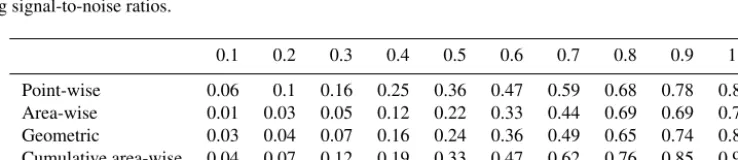
ofN (t ), andmis a number representing the signal-to-noise ratio. In the experiment, 100 different realizations of X(t ) were constructed by generating 100 realizations ofN (t ). The wavelet power spectrum of each realization ofX(t )was com-puted. The computations were repeated for values ofm rang-ing from 0.01 to 1.0. For each statistical test, the fraction of wavelet power coefficients statistically significant at a period of 8 was calculated for each realization. The mean fraction was then calculated for each value ofm, resulting in a curve representing how much of the signal on average is detected for different signal-to-noise ratios. Values close to 1.0 indi-cate that the test performed well at detecting the periodic sig-nal. For the experiments, the lag-1 autocorrelation coefficient was set to 0.1, 0.5, and 0.9, but only the results for 0.5 are dis-played because the results are only weakly dependent on the lag-1 autocorrelation coefficient. The point-wise, cumulative area-wise, and cumulative arc-wise tests were applied at the 5 % level, and the geometric and area-wise tests were applied at the 10 % level to 5 % point-wise significance regions.
As shown in Table A1, the amount of the signal detected by any of the tests increases as the signal-to-noise increases. Despite how the cumulative area-wise test is more strin-gent than the point-wise test, the tests detected a comparable amount of the signal for low to-noise ratios; for signal-to-noise ratios greater than 0.7, the test performed better. The cumulative arc-wise test outperformed the cumulative area-wise test for signal-to-noise ratios greater than 0.5. Consis-tent with theory, both the area-wise and geometric tests per-formed worse than the point-wise test. The performance of all tests was found to improve if the lag-1 autocorrelation co-efficients were increased to 0.9 and was found to worsen if the lag-1 autocorrelation coefficient was set to 0.1.
Table A1.The fraction of wavelet power coefficients at a period of 8 that are statistically significant in the case of a sinusoid embedded in noise with varying signal-to-noise ratios.
0.1 0.2 0.3 0.4 0.5 0.6 0.7 0.8 0.9 1.0
Supplement. The supplement related to this article is available online at: https://doi.org/10.5194/npg-26-91-2019-supplement.
Competing interests. The author declares that there is no conflict of interest.
Financial support. This research has been supported by the NASA Applied Sciences Project (grant no. NNX26AN38G).
Review statement. This paper was edited by Norbert Marwan and reviewed by two anonymous referees.
References
Adarsh, S. and Reddy M. J.: Trend analysis of rainfall in four me-teorological subdivisions of southern India using nonparamet-ric methods and discrete wavelet analysis, Int. J. Climatol., 35, 1107–1124, 2014.
Addison, P. S.: Wavelet transforms and the ECG: a review, Physiol. Meas., 26, R155, https://doi.org/10.1088/0967-3334/26/5/R01, 2005.
Agarwal, A., Maheswaran, R., Marwan, N., Caesar, L., and Kurths, J.: Wavelet-based multiscale similarity mea-sure for complex networks, Eur. Phys. J. B, 91, 296, https://doi.org/10.1140/epjb/e2018-90460-6, 2018.
Azad, S., Vignesh, T. S., and Narasimha, R.: Periodicities in Indian Monsoon Rainfall over spectrally homogeneous regions, Int. J. Climatol., 30, 2289–2298, 2010.
Edelsbrunner, H. and Harer, J.: Persistent homology-a survey, Con-temp. Math., 453, 257–282, 2008.
Elsanabary, M. H. and Gan, T. Y.: Wavelet analysis of seasonal rain-fall variability of the upper Blue Nile Basin, its teleconnection to Global Sea surface temperature, and its forecasting by an artifi-cial neural network, Mon. Weather Rev., 142, 1771–1791, 2014. Fasullo, J.: Biennial characteristics of All India rainfall, J. Climate,
17, 2972–2982, 2004.
Ferri, M.: Persistent topology for natural data analysis – A survey, in: Towards Integrative Machine Learning and Knowledge Ex-traction, Springer, Berlin/Heidelberg, Germany, 117–133, 2017. Gallegati, M.: A systematic wavelet-based exploratory analysis of
climatic variables, Climate Change, 148, 325–338, 2018. Grinsted, A., Moore, J. C., and Jevrejeva, S.: Application of the
cross wavelet transform and wavelet coherence to geophys-ical time series, Nonlin. Processes Geophys., 11, 561–566, https://doi.org/10.5194/npg-11-561-2004, 2004.
Hu, W. and Si, B. C.: Technical note: Multiple wavelet coherence for untangling scale-specific and localized multivariate relation-ships in geosciences, Hydrol. Earth Syst. Sci., 20, 3183–3191, https://doi.org/10.5194/hess-20-3183-2016, 2016.
Indian Institute of Tropical Meteorology: Meteorological Data Sets for Downloading, available at: https://www.tropmet.res.in/ DataArchival-51-Page, last access: 15 March 2019.
Kumar, P. and Foufoula-Georgiou, E.: Wavelet analysis for geo-physical applications, Rev. Geophys., 35, 385–412, 1997.
Labat, D.: Recent advances in wavelet analyses: Part 1. A review of concepts, J. Hydrol., 314, 275–288, 2005.
Labat, D.: Cross wavelet analyses of annual continental freshwater discharge and selected climate indices, J. Hydrol., 385, 269–278, 2010.
Lane, S. N.: Assessment of rainfall–runoff models based upon wavelet analysis, Hydrol. Process., 21, 586–607, 2007.
Lau, K.-M. and Weng, H.-Y.: Climate signal detection using wavelet transform: How to make a time series sing, B. Am. Meteorol. Soc., 76, 2391–2402, 1995.
Liu, Y., Liang, X. S., and Weisberg, R. H.: Rectification of the bias in the wavelet power spectrum, J. Atmos. Ocean. Tech., 24, 2093–2102, 2007.
Liu, Y., Brown, J., Demargne, J., and Seo, D.: A wavelet-based ap-proach to assessing timing errors in hydrological predictions, J. Hydrol., 397, 210–224, 2011.
Maheswaran, R. and Khosa, R.: A wavelet-based second order nonlinear model for forecasting monthly rainfall, Water Resour. Manag., 28, 5411–5431, 2014.
Maraun, D. and Kurths, J.: Cross wavelet analysis: significance testing and pitfalls, Nonlin. Processes Geophys., 11, 505–514, https://doi.org/10.5194/npg-11-505-2004, 2004.
Maraun, D., Kurths, J., and Holschneider, M.: Non-stationary Gaussian processes in wavelet domain: definitions, estima-tion and significance testing, Phys. Rev. E., 75, 016707, https://doi.org/10.1103/PhysRevE.75.016707, 2007.
Meyers, S. D., Kelly, B. G., and O’Brien, J. J.: An introduction to wavelet analysis in oceanography and meteorology: With appli-cation to the dispersion of Yanai waves, Mon. Weather Rev., 121, 2858–2866, 1993.
Narasimha, R. and Bhattacharyya, S.: A wavelet cross-spectral analysis of solar–ENSO–rainfall connections in the Indian mon-soons, Appl. Comput. Harmon. A., 28, 285–295, 2010. Nayagam, L. R., Janardanan, R., and Ram Mohan, H. S.:
Variabil-ity and teleconnectivVariabil-ity of northeast monsoon rainfall over India, Global Planet. Change, 69, 225–231, 2009.
Ng, E. K. W. and Chan, J. C. L.: Geophysical applications of par-tial wavelet coherence and multiple wavelet coherence, J. Atmos. Ocean. Tech., 29, 1845–1853, 2012.
NOAA/OAR/ESRL PSD: Climate Timeseries, available at: https: //www.esrl.noaa.gov/psd/gcos_wgsp/Timeseries/,last access: 15 March 2019.
Paluš, M.: Linked by Dynamics: Wavelet-Based Mutual In-formation Rate as a Connectivity Measure and Scale-SpecificNetworks, in: Advances in Nonlinear Geosciences, edited by: Tsonis, A. A., 427–463, Springer International Pub-lishing, Cham., 2018.
Parthasarathy B., Munot A. A., and Kothawale D. R.: All India monthly and seasonal rainfall series, 1871–1993, Theor. Appl. Climatol., 49, 217–224, 1994.
Parthasarathy, B., Munot, A. A., and Kothawale, D. R.: Monthly and seasonal rainfall series for all-India homogeneous regions and meteorological subdivisions: 1871–1994, Research Report No. RR-065, Indian Institute of Tropical Meteorology, Pune, 113 pp., 1995.
Ramana, R. V., Krishna, B., Kumar, S. R., and Pandey, N. G.: Monthly rainfall prediction using Wavelet Neural Network Anal-ysis, Water Resour. Manag., 27, 3697–3711, 2013.
Roy, I., Tedeschi, R. G., and Collins, M.: ENSO teleconnections to the Indian summer monsoon in observations and models, Int. J. Climatol., 37, 1794–1813, 2017.
Sahay, R. R. and Srivastava, A.: Predicting monsoon floods in rivers embedding wavelet transform, genetic algorithm and neural net-work, Water Resour. Manag., 28, 301–317, 2014.
Sang, Y. F.: A review on the applications of wavelet transform in hydrology time series analysis, Atmos. Res., 122, 8–15, 2012. Schaefli, B., Maraun, D., and Holschneider, M.: What drives high
flow events in the Swiss Alps? Recent developments in wavelet spectral analysis and their application to hydrology, Adv. Water Resour., 30, 2511–2525, 2007.
Schulte, J. A.: Cumulative areawise testing in wavelet analysis and its application to geophysical time series, Nonlin. Processes Geophys., 23, 45–57, https://doi.org/10.5194/npg-23-45-2016, 2016a.
Schulte, J. A.: Wavelet analysis for non-stationary, nonlin-ear time series, Nonlin. Processes Geophys., 23, 257–267, https://doi.org/10.5194/npg-23-257-2016, 2016b.
Schulte, J. A. and Georgas, N.: Theory and Practice of Phase-aware Ensemble Forecasting, Q. J. Roy. Meteor. Soc., 144, 1415–1428, 2018.
Schulte, J. A., Duffy, C., and Najjar, R. G.: Geometric and topologi-cal approaches to significance testing in wavelet analysis, Nonlin. Processes Geophys., 22, 139–156, https://doi.org/10.5194/npg-22-139-2015, 2015.
Schulte, J. A., Najjar, R. G., and Lee, S.: Salinity and Streamflow Variability in the Mid-Atlantic Region of the United States and its Relationship with Large-scale Atmospheric Circulation Pat-terns, J. Hydrol., 550, 65–79, 2017.
Terray, P., Delecluse, P., Labattu, S., and Terray, L.: Sea surface temperature associations with the late Indian summer monsoon, Clim. Dynam., 21, 593–618, 2003.
Torrence, C. and Compo, G. P.: A practical guide to wavelet analy-sis, B. Am. Meteorol. Soc., 79, 61–78, 1998.
Torrence, C. and Webster, P. J.: Interdecadal changes in the ENSO monsoon system, J. Climate, 12, 2679–2690, 1999.